Regional Forest Carbon Stock Estimation Based on Multi-Source Data and Machine Learning Algorithms

Abstract

Accurately assessing forest carbon stock (FCS) is essential for analyzing its spatial distribution and gauging the capacity of forests to sequester carbon. This research introduces a novel approach for estimating FCS by integrating multiple data sources, such as Sentinel-1 (S1) radar imagery, optical images from Sentinel-2 (S2) and Landsat 8 (L8), digital elevation modeling (DEM), and inventory data used in forest management and planning (FMP). Additionally, the estimation of FCS incorporates four key ecological features, including forest composition, primary tree species, humus thickness, and slope direction, to improve the accuracy of the estimation. Subsequently, insignificant features were eliminated using Lasso and recursive feature elimination (RFE) feature selection techniques. Three machine learning (ML) models were employed to estimate FCS: XGBoost, random forest (RF), and LightGBM. The results show that the inclusion of ecological information features improves the performance of the models. Among the models, LightGBM achieved superior performance (R² = 0.78, mean squared error (MSE) = 0.85, root mean squared error (RMSE) = 0.92, mean absolute error (MAE) = 0.58, relative RMSE (rRMSE) = 41.37%, and mean absolute percentage error (MAPE) = 30.72%), outperforming RF (R² = 0.76, MSE = 0.93, RMSE = 0.97, MAE = 0.60, rRMSE = 43.42%, and MAPE = 30.85%) and XGBoost (R² = 0.77, MSE = 0.90, RMSE = 0.95, MAE = 0.61, rRMSE = 42.66%, and MAPE = 34.61%).

1. Introduction

In response to the global climate crisis, international collaboration is essential to reduce greenhouse gas emissions, strengthen adaptation strategies, promote an economy focused on minimizing carbon output, and utilize natural carbon sinks, such as forests, to attain the 1.5 °C global temperature limit and reach net-zero emissions by 2050 [1,2,3]. Forests are essential to the global carbon cycle, holding about 45% of the carbon stored in terrestrial ecosystems across the globe [4]. Consequently, assessing FCS and monitoring the carbon balance are fundamental to meeting global climate goals [5]. With the intensification of climate change, accurately estimating FCS has become more critical in scientific research [6]. Obtaining long-term, continuous FCS data is essential for assessing the forest carbon sequestration capacity and provides a critical scientific basis for understanding ecosystem resilience [7].

Traditional carbon stock estimation methods rely on field sampling, measuring biomass by cutting down representative trees, and extrapolating carbon stocks for the entire forest based on scaling. However, these methods are time-consuming, labor-intensive, and can only provide limited ground-based data [8]. Remote sensing technologies enable the rapid and precise acquisition of forest data over extensive areas. By employing technologies such as optical remote sensing and synthetic aperture radar (SAR), in combination with the benefits of diverse remote sensing sources, it is possible to mitigate the limitations of a single data source and enhance the accuracy of carbon storage estimation [9,10].

Optical remote sensing technology frequently extracts vegetation indices and texture information, which, when combined with regression analysis, random forest, and other algorithms, help estimate FCS [11,12,13]. However, optical remote sensing is also subject to limitations, including susceptibility to clouds, smoke, aerosols, and other atmospheric conditions, and it struggles to capture information about the vertical structure of the forest [14]. In this context, active sensors, including SAR, serve as effective alternatives, capable of penetrating clouds and atmospheric disturbances, while offering essential insights into the forest’s vertical structure [14,15]. SAR offers unique advantages in estimating carbon stocks, particularly in dense forests, and can mitigate the saturation problem associated with optical data [16]. Although individual remote sensing data sources have limitations, combining optical and SAR data significantly enhances the accuracy of carbon stock estimations [17]. For instance, by combining S1 (SAR) and S2 (optical) data, researchers can develop more robust and accurate models for forest biomass (AGB) and aboveground carbon stock (AGC) [18,19]. Combining these two data sources not only leverages the rich spectral information provided by optical data but also capitalizes on the sensitivity of SAR data to a forest’s vertical structure, effectively overcoming the limitations associated with using one data source [17].

FCS estimation is affected by remote sensing data, as well as microenvironmental characteristics (e.g., soil texture, moisture, temperature, and humus thickness) and topographic factors (e.g., slope, aspect, etc.) [20,21]. Forest soil is the largest carbon reservoir on land worldwide, with microbial biomass playing a significant role and the physical and chemical characteristics of soil, both of which play a crucial role in the decomposition and stock of carbon. [22]. Moreover, the stock of carbon in soil is affected by multiple environmental factors. Factors like temperature and precipitation control microbial activity, thereby affecting carbon dynamics. Studies have demonstrated that topographic factors, including aspect and slope, significantly impact FCS [23]. For instance, soil carbon stock on slopes with little sunlight tends to be higher than on slopes with direct sunlight, while areas with steeper slopes are more prone to soil erosion, which, in turn, influences carbon stock [24]. Forest composition, primary tree species, and tree age significantly influence carbon stock [25,26]. Older forests typically store more carbon due to greater biomass accumulation and enhanced soil carbon sequestration [27]. The species composition and plant diversity of understory vegetation also play a role in carbon stock [28]. Understanding these microenvironmental and topographical features is critical for optimizing silvicultural practices and enhancing carbon stock estimates.

In recent years, the use of ML for carbon stock estimation has advanced considerably. In addition to traditional regression analysis, modern ML algorithms—like artificial neural networks (ANNs), support vector regression (SVR), random forests (RF), deep learning (DL), and ensemble learning (EL)—are increasingly applied in FCS estimation [29,30]. These algorithms can effectively model complex nonlinear relationships, thereby significantly enhancing the precision and reliability of the models. In particular, boosting algorithms, like Light Gradient Boosting Machine (LightGBM) and Extreme Gradient Boosting (XGBoost), are particularly effective in smaller sample cases and have demonstrated high accuracy in FCS estimation [31,32].

This study utilizes multi-source remote sensing data, including S1 radar imagery, S2 optical imagery, L8 optical imagery, and DEM, to develop a carbon stock estimation model. In addition to these datasets, ecological information (such as forest composition and primary tree species) and environmental factors (such as humus depth and slope direction) are incorporated to refine the model accuracy. For optimal feature selection, this study employs the least absolute shrinkage and selection operator (Lasso) and recursive feature elimination (RFE) methods to identify critical independent variables. Furthermore, three machine learning models—LightGBM, XGBoost, and random forest (RF)—are implemented to estimate FCS. By assessing a range of performance metrics, this study determines the most effective data integration sources and algorithms to enhance estimation precision.

2. Materials and Methods

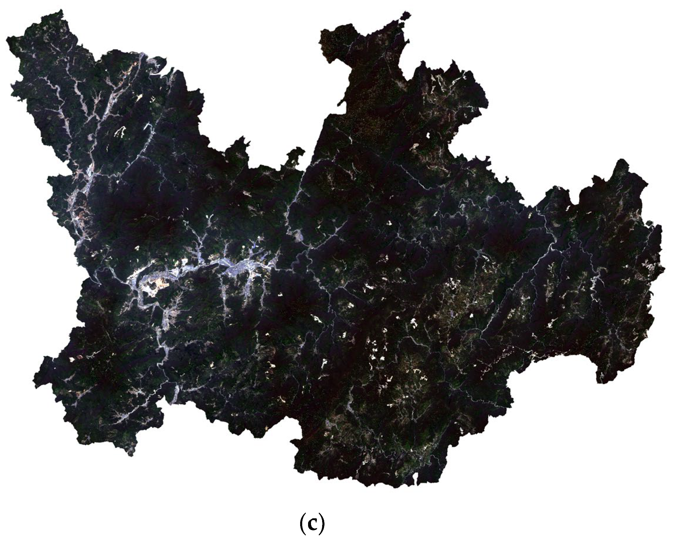
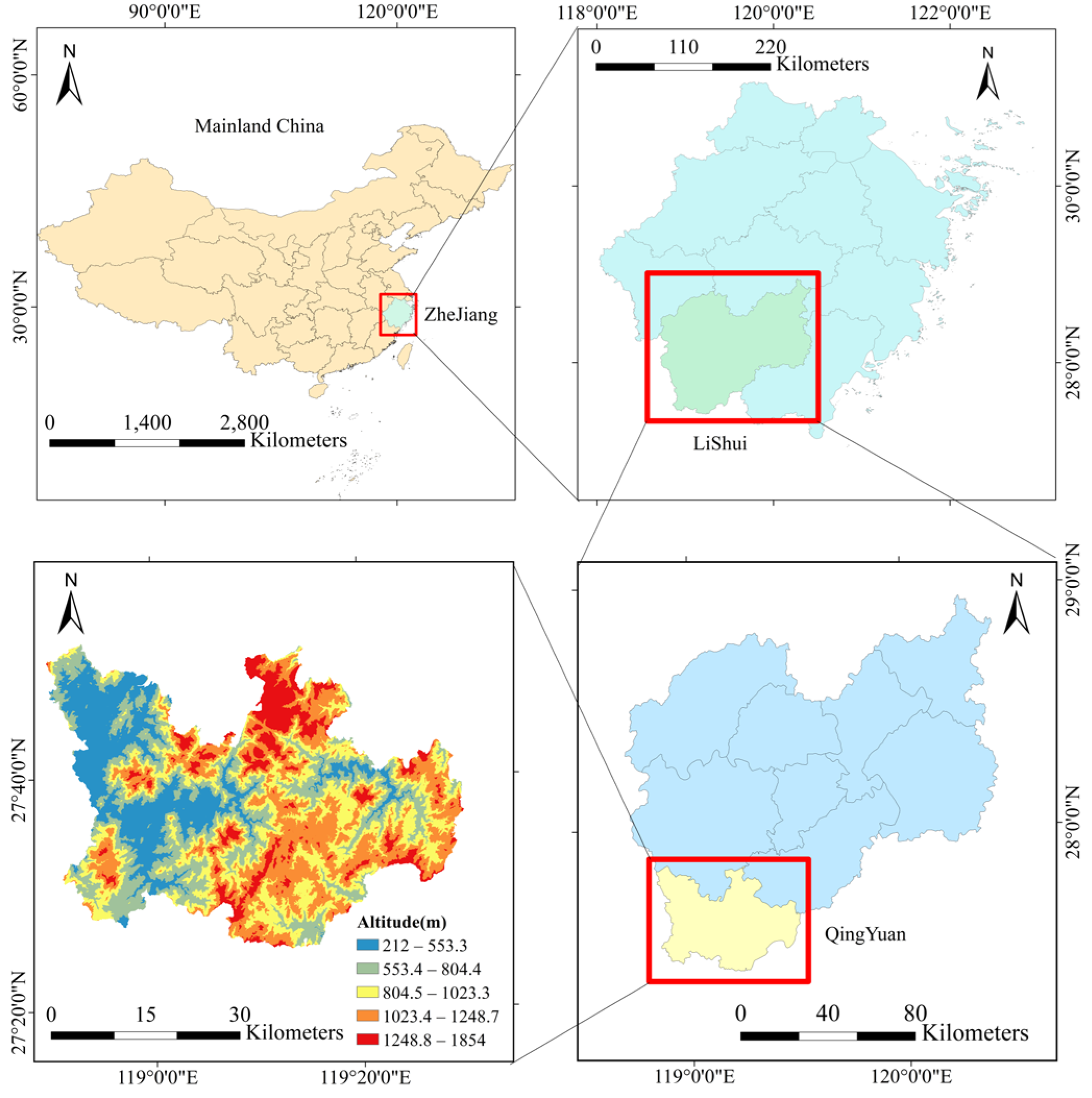
2.1. Introduction to the Research Area

Qingyuan County is located in the southwestern mountainous area of Zhejiang Province, with geographical coordinates ranging from 27°25′ to 27°51′ N and 118°50′ to 119°30′ E. The area is characterized by a variety of landforms, including valleys, basins, hills, and low- to medium-altitude mountains. The county boasts 23 peaks that exceed an elevation of 1500 m; among which, the main peak, Baishanzu, reaches 1856.7 m above sea level, ranking it as the second tallest in Zhejiang Province. The lowest point in the county is located in Xinyao Village, with an altitude of 240 m. Qingyuan County enjoys a warm and humid subtropical monsoon climate, noted for its mild winters and moderate summers. The region has an annual average temperature of 17.4 °C, receives 1760 mm of precipitation annually, and has a frost-free period lasting 245 days. The predominant natural vegetation is evergreen broadleaf forest, and the main forest types include evergreen broadleaf forests and coniferous forests. As of 2017, Qingyuan County encompasses a total land area of 189,780 ha, of which 168,267 ha are forested, and the forest coverage rate is 86%. Recent studies have indicated that the FCS in Lishui City, where Qingyuan County is located, ranged from 0.21 Mg C ha⁻¹ to 69.58 Mg C ha⁻¹ in 2019 [33]. The specific location of the study area is illustrated in Figure 1.

2.2. Research Data and Methods

2.2.1. Research Data

The ground data for this study include a DEM (refer to Figure 1) and FMP published by the Lishui Forestry Bureau in 2017. The data encompass 38,994 samples of forest sub-compartments within Qingyuan County, offering comprehensive details on forest resources. The DEM is sourced from version 2 of the global digital elevation model (ASTER GDEM), featuring a 30-m resolution, and the World Geodetic System 1984 (WGS84) coordinate system. This dataset, released in 2017, is available from the International Science and Technology Data Mirror Site of the Computer Network Information Center of the Chinese Academy of Sciences and covers a single scene. Through ArcGIS, the DEM image data underwent coordinate system conversion, splicing, and clipping to extract three terrain factors: altitude, slope, and aspect.

The optical remote sensing image data consist of S2 satellite imagery from the European Space Agency’s Copernicus program and L8 Operational Land Imager (OLI) images. The S2 imagery was captured on 25 December 2017 using L2-A image data. The L8 OLI data were acquired on 3 November 2017. Both images were acquired under favorable meteorological conditions, with cloud cover below 10%. The images exhibited high spatial clarity and data availability, ensuring reliable support for related research [34].

The radar remote sensing images were obtained from the S1 satellite, with SAR imaging conducted on 10 December 2017, using IW GRD-level data. The specifications and acquisition dates of the remote sensing dataset are detailed in

Table 1. Specifications and acquisition dates of the remote sensing dataset.

Types	Satellite	Date	Product Level
Optical remote sensing	Sentinel-2A	25 December 2017, 1 scene	L2A
	Landsat 8	3 November 2017, 1 scene	L1TP
Radar remote sensing	Sentinel-1A	10 December 2017, 1 scene	IW GRD

, and all remote sensing images employ the WGS84 coordinate system. The preprocessed S1, S2, and L8 remote sensing images are presented in Figure A1.

In this study, the L8 image was acquired on 3 November 2017, and the Sentinel-2A (S2A) image was acquired on 25 December 2017. Although the nearly two-month difference may theoretically impact the carbon model’s accuracy, the impact is minimal. Firstly, Zhejiang’s subtropical monsoon climate, characterized by mild winters, leads to minimal seasonal vegetation changes. The primary species of trees in the study area, including Pinus massoniana Lamb and Abies, exhibit slow growth during autumn and winter. Quercus and Betula, which enter dormancy, comprise only 1% of the area and have a negligible impact on the carbon stock estimation [35,36]. Secondly, the remote sensing data underwent rigorous atmospheric correction using standard methods such as Sen2Cor and LaSRC, minimizing the errors caused by the time difference. The model also incorporated data from different time windows during training, enhancing its robustness and adaptability. Therefore, the time difference between the L8 and S2 image acquisitions has minimal impact on the carbon model’s accuracy, an effect that can be further mitigated through subsequent error control and model optimization.

For Sentinel-2B (S2B) Level 2-A product image data preprocessing, SNAP software was employed to resample the images. The resampling specifications included a 10-m output resolution, with the “Nearest” method for upsampling, the “Mean” method for general downsampling, and the “First” method for labeled data downsampling. Additionally, pyramid-based resampling was enabled to accelerate image processing, enhancing the spatial data consistency and processing efficiency. The preprocessed images were subsequently cropped using the administrative vector map of Qingyuan County to match Qingyuan County’s boundaries. The L8 images underwent radiation calibration and atmospheric correction in ENVI software (Version 5.6) to reduce atmospheric interference, followed by cropping based on Qingyuan County’s administrative vector map.

The S1 radar system, known for its vector characteristics, operates in four polarization modes: HH, VV, HV, and VH. The VV-VH mode is typically used for terrestrial observation, while HH-HV and HH modes are chiefly applied to monitor polar environments. This study utilized S1 radar images in IWGRD mode (TOPS Mode), with VV and VH polarization modes in the ascending orbit [37].

Preprocessing of the radar images in SNAP involved thermal noise removal, speckle filtering, radiation calibration, and terrain correction to address noise, radiation, and terrain-related errors. The images were cropped afterward to the administrative boundary of Qingyuan County. Remote sensing information was extracted from the VV and VH polarization modes of the S1 image to detail the surface features and ensure data reliability for subsequent analysis.

To extract surface texture features, a 3 × 3 pixel sliding window approach was applied at a 45° fixed direction and a 1-pixel step size. Eight key texture features were computed using VV and VH backscattering coefficients: mean, homogeneity, entropy, dissimilarity, contrast, correlation, variance, and second moment.

2.2.2. Calculation of the Carbon Stock

In this study, the sample plot’s carbon stock was estimated using a biomass-based carbon stock model. Initially, the biomass of tree species i was calculated using the following Formulas (1)–(3) [38], as given below:

$${\mathrm{B}}_{\mathrm{T}\mathrm{R}\mathrm{E}\mathrm{E},\mathrm{i}}={\mathrm{V}}_{\mathrm{T}\mathrm{R}\mathrm{E}\mathrm{E}\mathrm{M},\mathrm{i}}\times {\mathrm{D}}_{\mathrm{T}\mathrm{R}\mathrm{E}\mathrm{E},\mathrm{i}}\times {\mathrm{B}\mathrm{E}\mathrm{F}}_{\mathrm{T}\mathrm{R}\mathrm{E}\mathrm{E}.\mathrm{i}}\times \left(1+{\mathrm{R}}_{\mathrm{T}\mathrm{R}\mathrm{E}\mathrm{E},\mathrm{i}}\right)\times {\mathrm{N}}_{\mathrm{T}\mathrm{R}\mathrm{E}\mathrm{E},\mathrm{i}}\times \mathrm{A}$$

(1)

At the same time, according to Formula (2), the carbon stock of tree species i can be derived by multiplying its biomass with the carbon conversion coefficient:

$${\mathrm{C}}_{\mathrm{T}\mathrm{R}\mathrm{E}\mathrm{E},\mathrm{i}}={\mathrm{B}}_{\mathrm{T}\mathrm{R}\mathrm{E}\mathrm{E},\mathrm{i}}\times {\mathrm{C}\mathrm{F}}_{\mathrm{T}\mathrm{R}\mathrm{E}\mathrm{E},\mathrm{i}}$$

(2)

Combining the above two equations, the carbon stock of tree species i is directly expressed as follows:

$${\mathrm{C}}_{\mathrm{T}\mathrm{R}\mathrm{E}\mathrm{E},\mathrm{i}}={\mathrm{V}}_{\mathrm{T}\mathrm{R}\mathrm{E}\mathrm{E},\mathrm{i}}\times {\mathrm{D}}_{\mathrm{T}\mathrm{R}\mathrm{E}\mathrm{E},\mathrm{i}}\times {\mathrm{B}\mathrm{E}\mathrm{F}}_{\mathrm{T}\mathrm{R}\mathrm{E}\mathrm{E}.\mathrm{i}}\times \left(1+{\mathrm{R}}_{\mathrm{T}\mathrm{R}\mathrm{E}\mathrm{E},\mathrm{i}}\right)\times {\mathrm{C}\mathrm{F}}_{\mathrm{T}\mathrm{R}\mathrm{E}\mathrm{E},\mathrm{i}}\times {\mathrm{N}}_{\mathrm{T}\mathrm{R}\mathrm{E}\mathrm{E},\mathrm{i}}\times \mathrm{A}$$

(3)

here:

• ${\mathrm{B}}_{\mathrm{T}\mathrm{R}\mathrm{E}\mathrm{E},\mathrm{i}}$: biomass of tree species i, in tons of dry weight;
• ${\mathrm{V}}_{\mathrm{T}\mathrm{R}\mathrm{E}\mathrm{E},\mathrm{i}}$: standing timber volume of tree species i, measured in cubic meters per plant;
• ${\mathrm{D}}_{\mathrm{T}\mathrm{R}\mathrm{E}\mathrm{E},\mathrm{i}}$: basic wood density of tree species i, in tons of dry weight per cubic meter;
• ${\mathrm{B}\mathrm{E}\mathrm{F}}_{{\mathrm{s}\mathrm{p}\mathrm{e}\mathrm{c}\mathrm{i}\mathrm{e}\mathrm{s}}_{\mathrm{i}}}$: aboveground biomass expansion factor of tree species i, a dimensionless parameter;
• ${\mathrm{R}}_{\mathrm{T}\mathrm{R}\mathrm{E}\mathrm{E},\mathrm{i}}$: the belowground-to-aboveground biomass ratio for tree species i;
• $\mathrm{B}\mathrm{C}{\mathrm{E}\mathrm{F}}_{\mathrm{T}\mathrm{R}\mathrm{E}\mathrm{E},\mathrm{i}}$: conversion and expansion factor of the biomass of tree species i, in tons of dry weight per cubic meter;
• ${\mathrm{N}}_{\mathrm{T}\mathrm{R}\mathrm{E}\mathrm{E},\mathrm{i}}$: number of trees of tree species i, expressed as the number of trees per hectare;
• A: the area of the corresponding sub-compartments, in hectares.

The calculation process initiated with field survey data to ascertain the tree stock volume for each forest sub-compartment. Subsequently, the aboveground biomass was computed by integrating the wood density of the various tree species with their respective biomass expansion factors. The biomass values were hence translated into carbon stock using the carbon conversion coefficient. An estimation of the carbon stock within the underground root system was derived from the underground-to-aboveground biomass ratio, leading to the aggregate carbon stock for each tree species (details provided in

Table 2. Calculation method of carbon storage of various tree species in Qingyuan County.

Species	Model	Reference
Pinus massoniana Lamb	C = V × 0.380 × 1.472 × 0.508 × 1.187 × N × A	[38]
Secondary Pinus species	C = V × 0.424 × 1.631 × 0.496 × 1.206 × N × A
Abies	C = V × 0.307 × 1.634 × 0.508 × 1.246 × N × A
Quercus	C = V × 0.676 × 1.355 × 0.499 × 1.292 × N × A
Betula	C = V × 0.541 × 1.424 × 0.502 × 1.248 × N × A
Liquidambar	C = V × 0.598 × 1.765 × 0.480 × 1.398 × N × A
Hard broadleaf	C = V × 0.598 × 1.674 × 0.496 × 1.261 × N × A
Soft broadleaf	C = V × 0.443 × 1.586 × 0.486 × 1.289 × N × A
Mixed coniferous-broadleaf forest	C = V × 1.514 × 0.482 × 0.5 × 1.289 × N × A

Note: In the models in the table, C represents carbon storage, V represents stock volume, N represents the number of plants per hectare, and A represents the sub-compartment area.

). This model encompassed both aboveground and underground biomass carbon stock, thereby offering a more precise representation of FCS.

In order to ensure data accuracy, the initial dataset of 38,994 samples of forest sub-compartments was refined by filtering out non-forest plots, samples with zero volume or canopy density, and outliers identified through the interquartile range (IQR) method [39]. After this data purification process, 36,187 valid samples were retained for analysis. These samples encompassed 10 primary tree species, including Abies, mixed coniferous-broadleaf forests, Quercus, soft broadleaf, Pinus massoniana, secondary Pinus species, mixed coniferous-broadleaf, Betula, and other tree species. Figure 2 provides a detailed illustration of carbon stock per hectare for each forest sub-compartment.

2.3. Extraction of Independent Variable Factors

2.3.1. Optical Remote Sensing Factors

This study employs L8 image data, known for its comprehensive coverage of global land and oceanic regions, as the basis for the carbon stock estimation model. The L8 dataset includes nine Operational Land Imager (OLI) bands and two Thermal Infrared Sensor (TIRS) bands, as outlined in

Table A1. Characteristics of the spectral bands in L8.

Band Number	Name	Wavelength Range (µm)	Spatial Resolution (m)	Main Applications
B1	Aerosol	0.433–0.453	30	Atmospheric correction, shallow water and coastal monitoring
B2	Blue	0.450–0.515	30	Water monitoring, vegetation health, soil/water comparisons
B3	Green	0.525–0.600	30	Vegetation health analysis, agriculture and forest monitoring
B4	Red	0.630–0.680	30	Vegetation analysis (NDVI calculation), land cover classification
B5	NIR	0.845–0.885	30	Vegetation analysis, land cover monitoring, water body boundary identification
B6	SWIR 1	1.560–1.660	30	Soil and vegetation moisture content, farmland irrigation monitoring
B7	SWIR 2	2.100–2.300	30	Geological feature analysis, mineral exploration, vegetation pressure
B8	Panchromatic	0.500–0.680	15	High-resolution image fusion and linear feature extraction
B9	Cirrus	1.360–1.390	30	Thin cloud detection
B10	TIRS 1	10.60–11.19	100	Surface temperature monitoring, thermal characteristics analysis
B11	TIRS 2	11.50–12.51	100	Surface temperature monitoring, thermal activity analysis

. For the purposes of this study, the first seven bands (B1–B7) of the L8 images were chosen as independent variables for the carbon stock estimation model. These bands facilitate the extraction of key vegetation attributes related to carbon stock, such as health, density, and coverage, spanning the visible spectrum (B2, B3, and B4); the near-infrared spectrum (B5); and the short-wave infrared spectrum (B6 and B7). This selection effectively captures the spectral properties of surface vegetation, water bodies, and soil.

Among the spectral bands, the visible spectral bands (B2, B3, and B4) are mainly employed to extract the color and reflection features of vegetation in carbon stock prediction, which effectively reflect the chlorophyll content, vegetation health, and changes in vegetation coverage. This provides an important reference for assessing vegetation growth and carbon fixation capacity. The near-infrared band (B5) is essential for vegetation health assessment and biomass estimation, offering key support for the indirect estimation of carbon stock. The short-wave infrared bands (B6 and B7) are critical for assessing vegetation moisture, biomass, and soil moisture content, which are key to carbon stock estimation. Additionally, the coastal aerosol band (B1) enhances the image data quality and model prediction accuracy by reducing the atmospheric aerosol interference. This band combination not only efficiently extracts spectral information but also streamlines data processing and enhances the reliability and accuracy of carbon stock predictions [40].

In contrast, the bands not selected for the model have limited applicability to carbon stock estimation and could complicate data processing. For instance, the panchromatic band (B8), which primarily covers the visible spectrum and is used for image sharpening, lacks the necessary vegetation spectral information for carbon stock estimation. The cirrus band (B9), while useful for atmospheric correction, does not directly provide spectral data on surface vegetation or soil. Similarly, the thermal infrared bands (B10 and B11), used mainly for surface temperature monitoring, have lower resolution and are less suitable for the demands of carbon stock estimation. Therefore, the choice of B1–B7 as input variables constitutes a straightforward and effective strategy that enhances the accuracy and performance of the carbon stock estimation model.

Meanwhile, this study extracted two types of independent variables from S2 optical remote sensing images: original (Bands 1–9, 8A, 11, and 12) and derived factors (such as the vegetation indices listed in

Table 3. Vegetation index calculation based on Sentinel-2 multispectral bands.

No.	Variable Name	Formula	Reference
1	Soil Adjusted Vegetation Index (SAVI)	SAVI = ((B8 − B4)/(B8 + B4 + L)) × 1.5	[43]
2	Ratio Vegetation Index (RVI)	RVI = B8/B4	[44]
3	Nonlinear Index (NLI)	NLI = ((B8 × B8) − B4)/((B8 × B8) + B4)	[45]
4	Normalized Difference Vegetation Index (NDVI)	NDVI = (B8 − B4)/(B8 + B4)	[46]
5	Modified Normalized Difference Vegetation Index (mNDVI)	mNDVI = (B8 − B4)/(B8 + B4−2 × B2)	[47]
6	Normalized Difference Infrared Index (NDII)	NDII = (B8 − B11)/(B8 + B11)	[48]
7	Normalized Difference Green Index (NDGI)	NDGI = (B3 − B4)/(B3 + B4)	[49]
8	Enhanced Vegetation Index (EVI)	EVI = 2.5 × (B8 − B4)/(B8 + 6 × B4−7.5 × B2 + 1)	[50]
9	Difference Vegetation Index (DVI)	DVI = B8 − B4	[51]
10	RedEdge Ratio Vegetation Index (RVIre)	RVIre = B8/B5	[52]
11	RedEdge1 Normalized Difference Vegetation Index (NDVIre1)	NDVIre1 = (B8 − B5)/(B8 + B5)	[53]
12	RedEdge2 Normalized Difference Vegetation Index (NDVIre2)	NDVIre2 = (B8 − B6)/(B8 + B6)	[53]
13	Modified RedEdge Normalized Difference Vegetation Index (mNDVIre)	mNDVIre = (B8 − B5)/(B8 + B5-2 × B2)	[47]
14	RedEdge Nonlinear index (NLIre)	NLIre = ((B8 × B8) − B5)/((B8 × B8) + B5)	[52]

Note: The indices in this table are calculated based on Sentinel-2 bands (B1–B12), where bands 1 to 8 are used for calculations. The band data are from Sentinel-2 satellite images and are referenced in each vegetation index formula.

). The original factors include 12 bands, covering spectral information from coastal to short-wave infrared ranges, offering comprehensive data for estimating FCS [41,42]. Notably, the B10 band of the S2 images is primarily used for cloud detection and atmospheric correction, making it unsuitable for direct use in FCS inversion. However, during data preprocessing, the B10 band enhances the quality of other bands through cloud detection and atmospheric correction, indirectly improving the accuracy of carbon stock inversion.

2.3.2. Extraction of Dual-Polarization Texture Features from Radar Backscattering Coefficients

According to the backscattering coefficients corresponding to VV and VH polarization, eight typical texture features, including mean, homogeneity, entropy, dissimilarity, contrast, correlation, variance, and second-order moment, are calculated, totaling 16 key texture feature variables. These feature variables together constitute the input for the subsequent analysis, providing multi-angle and multi-dimensional texture information support for the model [54].

2.3.3. Independent Variable Factors from Ground Data

Based on FMP, the study considered twelve independent variables: land type, landforms, soil type, soil thickness, slope position, vegetation coverage, tree age, canopy density, forest composition, primary tree species, humus thickness, and aspect direction. Furthermore, the DEM yielded three additional independent variables: elevation, slope, and aspect.

2.3.4. Data Integration

Integrating the factors outlined in Section 2.3.1, Section 2.3.2 and Section 2.3.3, a comprehensive set of 64 independent variables was assembled (as detailed in

Table 4. Feature lists from multi-source remote sensing data and FMP.

No.	Factor Name	Source of Data	Types of Factors
1–19	Band reflectance	Optical Remote Sensing	Independent Variable Factors
20–33	Refer to Table 3	Vegetation indexes
34–35 36–37	Mean	Radar Remote Sensing
	Variance
38–39	Homogeneity
40–41	Contrast
42–43	Dissimilarity
44–45	Entropy
46–47	Angular second moment
48–49	Correlation
50	ELEVATION	Digital Elevation Model
51	SLOPE
52	ASPECT
53	Land Type	Inventory Data used in Forest Management and Planning
54	Landforms
55	Soil Type
56	Soil Thickness
57	Slope Position
58	Vegetation Coverage
59	Tree Age
60	Canopy Density
61	Forest Composition	Inventory Data used in Forest Management and Planning	Ecological information features
62	Primary Tree Species
63	Humus Thickness
64	Aspect Direction

). For modeling and predictive purposes, all preprocessed data—encompassing FMP; DEM; and remote sensing imagery from L8, S2, and S1— were merged into a unified dataset. This database was structured with the forest sub-compartment as the fundamental unit, and 36,187 samples were employed in this study, with 80% (28,949) allocated for training and 20% (7238) reserved for testing.

2.4. Methods

2.4.1. XGBoost

XGBoost is an advanced ensemble ML algorithm that builds upon gradient-boosted decision trees (GBDTs) [55]. Its fundamental approach involves establishing an initial base classifier or regressor, to which new models are sequentially added to enhance performance. Each addition recalculates the objective function, incrementally refining the model’s fit. XGBoost stands out for its strong generalization capabilities, achieved through the inclusion of regularization terms in the objective function to prevent overfitting, distinguishing it from conventional GBDT methods.

2.4.2. RF

RF is a renowned bagging ensemble learning method that generates predictions by creating multiple decision trees and aggregating their outcomes [56]. In this approach, each decision tree independently predicts the target variable, and the final prediction is computed by averaging the forecasts from each tree in the model. This method effectively reduces the inter-tree correlation and model variance, thereby enhancing the prediction accuracy. The strength of RF lies in its ability to handle datasets with high-dimensional features, demonstrating high adaptability and sensitivity.

2.4.3. LightGBM

LightGBM is a gradient boosting framework that leverages decision trees optimized for large-scale datasets and high-dimensional sparse features [32]. As part of the gradient boosting model family, LightGBM leverages the strengths of the algorithm by constructing multiple weak learners (typically decision trees) to improve the overall model performance.

2.4.4. Lasso

Lasso serves as a method for feature selection frequently used for variable screening in high-dimensional datasets. By incorporating an L1 regularizer, Lasso drives the coefficients of non-informative features to zero, effectively excluding them from the model. Lasso offers notable advantages in efficiency and stability over other feature selection techniques [57].

2.4.5. RFE

By constructing a model, RFE eliminates the least important features in stages based on their weights, thereby uncovering the key predictors. This method involves training the model, evaluating feature importance in each iteration, and iteratively discarding the least important features until the desired feature count is attained or the performance benchmarks of the model are fulfilled [58].

2.5. Performance Indicators

To facilitate model convergence, the min–max normalization method is used to scale all features to a 0 to 1 range, reflecting their individual value ranges. Subsequently, random allocation divides the samples into an 80% training set and a 20% testing set [59,60]. Ten-fold cross-validation is employed during training to fine-tune the parameters. The validation set is utilized afterward to compute the evaluation metrics, including root mean squared error (RMSE), the coefficient of determination (R²), mean absolute percentage error (MAPE), mean absolute error (MAE), mean squared error (MSE), and relative root mean squared error (rRMSE). The accuracy of the evaluation model is determined using Formulas (4)–(9):

$${\mathrm{R}}^2={\displaystyle \frac{{\sum }_{\mathrm{i}=1}^{\mathrm{n}}{({\widehat{\mathrm{y}}}_{\mathrm{i}}-\overline{\mathrm{y}})}^2}{{\sum }_{\mathrm{i}=1}^{\mathrm{n}}{({\mathrm{y}}_{\mathrm{i}}-\overline{\mathrm{y}})}^2}}$$

(4)

$$\mathrm{R}\mathrm{M}\mathrm{S}\mathrm{E}=\sqrt{{\displaystyle \frac{1}{\mathrm{n}}}{\sum }_{\mathrm{i}=1}^{\mathrm{n}}{\left({\widehat{\mathrm{y}}}_{\mathrm{i}}-{\mathrm{y}}_{\mathrm{i}}\right)}^2}$$

(5)

$$\mathrm{M}\mathrm{S}\mathrm{E}={\displaystyle \frac{1}{\mathrm{n}}}\sum _{\mathrm{i}=1}^{\mathrm{n}}{\left({\stackrel{\mathrm{ˆ}}{\mathrm{y}}}_{\mathrm{i}}-{\mathrm{y}}_{\mathrm{i}}\right)}^2$$

(6)

$$\mathrm{M}\mathrm{A}\mathrm{E}={\displaystyle \frac{1}{\mathrm{n}}}\sum _{\mathrm{i}=1}^{\mathrm{n}}\left|\left({\stackrel{\mathrm{ˆ}}{\mathrm{y}}}_{\mathrm{i}}-{\mathrm{y}}_{\mathrm{i}}\right)\right|$$

(7)

$$\mathrm{M}\mathrm{A}\mathrm{P}\mathrm{E}={\displaystyle \frac{1}{\mathrm{n}}}\sum _{\mathrm{I}=1}^{\mathrm{n}}{\displaystyle \frac{\left|\left({\stackrel{\mathrm{ˆ}}{\mathrm{y}}}_{\mathrm{i}}-{\mathrm{y}}_{\mathrm{i}}\right)\right|}{{\mathrm{y}}_{\mathrm{i}}}}\times 100\mathrm{\%}$$

(8)

$$\mathrm{r}\mathrm{R}\mathrm{M}\mathrm{S}\mathrm{E}={\displaystyle \frac{\mathrm{R}\mathrm{M}\mathrm{S}\mathrm{E}}{\overline{\mathrm{y}}}}\times 100\mathrm{\%}$$

(9)

Specifically, ${\mathrm{y}}_{\mathrm{i}}$ is the measured carbon stock, ${\overline{\mathrm{y}}}_{\mathrm{i}}$ is the average of the measured carbon stocks, ${\widehat{\mathrm{y}}}_{\mathrm{i}}$ is the predicted carbon stock, $\mathrm{i}$ indicates the sample number, and $\mathrm{n}$ denotes the total number of samples.

3. Results

Four data schemes—A, B, C, and D—were developed based on two feature selection methods: RFE and Lasso and whether or not ecological information features were included, as detailed in

Table 5. Data schemes.

Data Scheme	Feature Selection Method	Ecological Information Features	Total Number of Initial Features
A	RFE	Did not add	60
B	RFE	Added	64
C	Lasso	Did not add	60
D	Lasso	Added	64

.

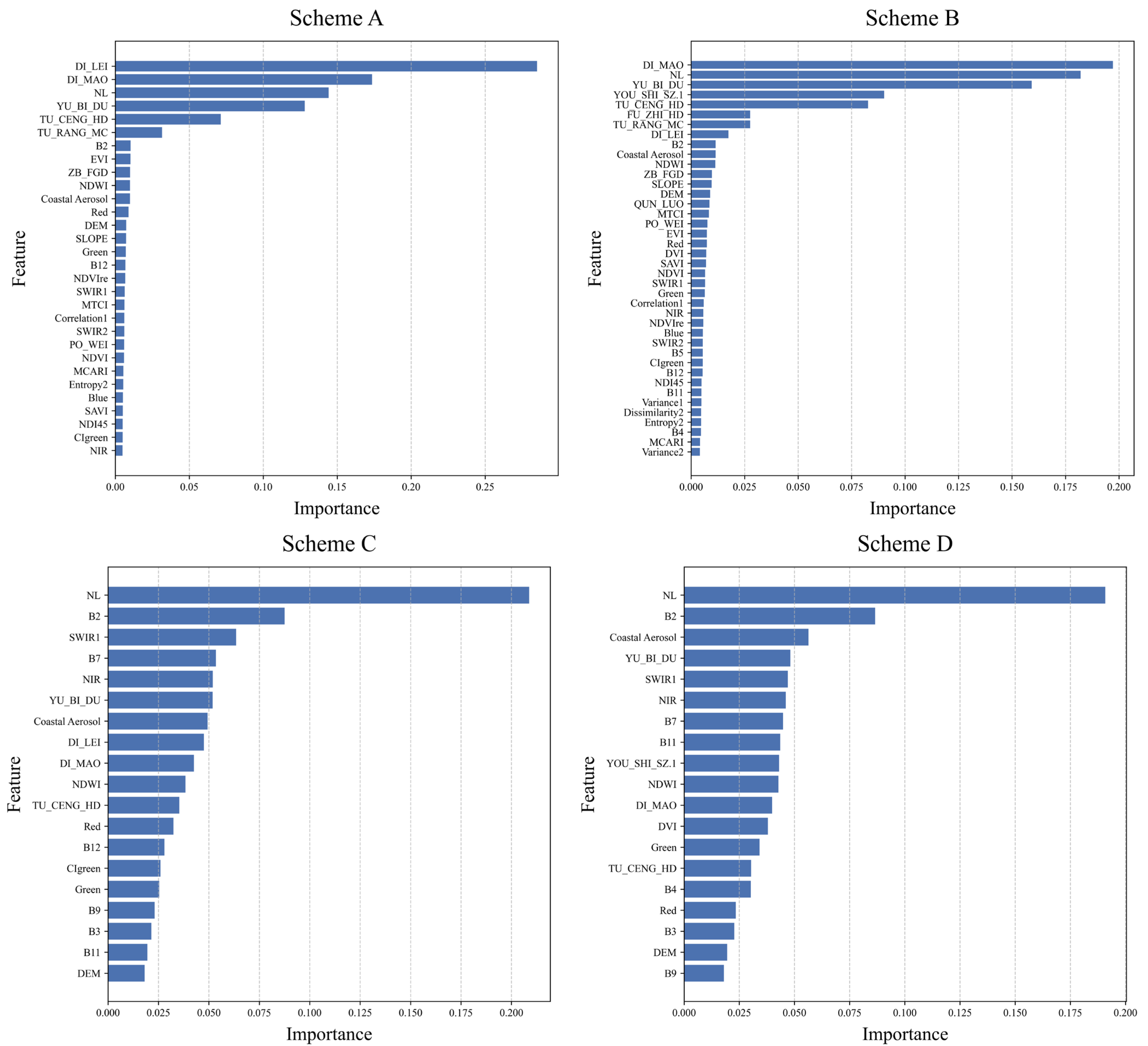
3.1. Screening for Independent Variable Factors

Data schemes A and C, which incorporate S1, S2, L8, DEM, and forest resource planning data, initially identified 60 numerical features. The RFE and Lasso methods were subsequently applied to select key variables. Scheme A, using RFE, retained 30 features, while scheme C, employing Lasso (alpha = 0.001, threshold = 0.1), selected 19 features. For schemes B and D, four ecological information features were incorporated, bringing the total to 64. The feature selection methods and parameters for schemes B and D mirrored those of schemes A and C. Scheme B retained 40 features, while scheme D retained 19. The results for all schemes are presented in Figure 3.

3.2. Results Analysis

This research investigates how two feature selection methods (RFE and Lasso) shape the feature selection process. It also investigates the effect of incorporating ecological information features on the performance of different ML algorithms, including XGBoost, RF, and LightGBM.

Table 6. Evaluation metrics for FCS estimation derived from the data schemes.

Data Scheme		A	B	C	D
XGBoost	MSE	1.01	0.90	1.04	0.95
	RMSE (t/ha)	1.01	0.95	1.02	0.97
	MAE (t/ha)	0.65	0.61	0.66	0.63
	R2	0.74	0.77	0.73	0.75
	rRMSE (%)	45.29	42.66	45.90	43.79
	MAPE (%)	39.29	34.61	40.01	38.11
RF	MSE	1.01	0.93	1.02	0.94
	RMSE (t/ha)	1.00	0.97	1.01	0.97
	MAE (t/ha)	0.63	0.60	0.64	0.60
	R2	0.74	0.76	0.73	0.76
	rRMSE (%)	45.17	43.42	45.45	43.54
	MAPE (%)	33.73	30.85	34.11	30.77
LightGBM	MSE	0.97	0.85	0.99	0.88
	RMSE (t/ha)	0.99	0.92	1.00	0.94
	MAE (t/ha)	0.63	0.58	0.64	0.59
	R2	0.75	0.78	0.74	0.77
	rRMSE (%)	44.34	41.37	44.79	42.11
	MAPE (%)	34.77	30.72	34.74	31.19

presents the performance metrics for the FCS estimation model across the four data schemes.

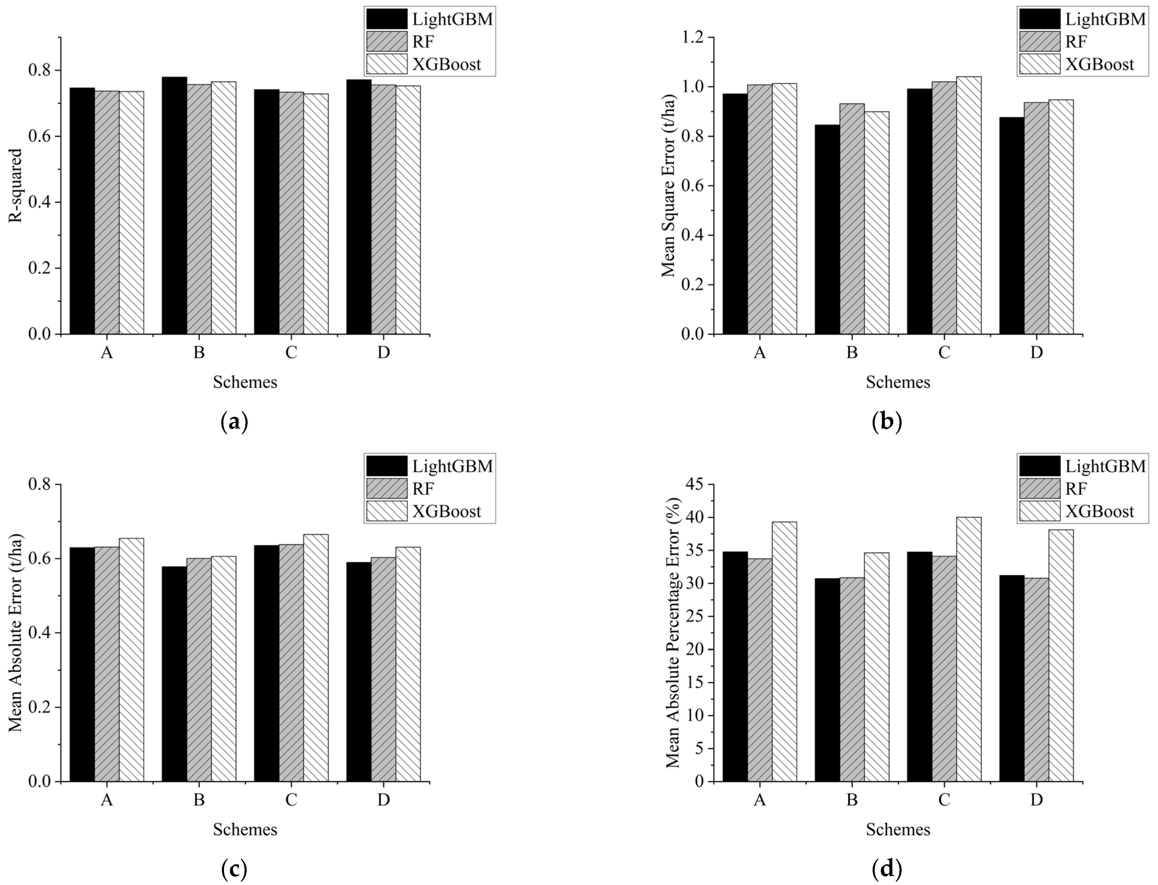
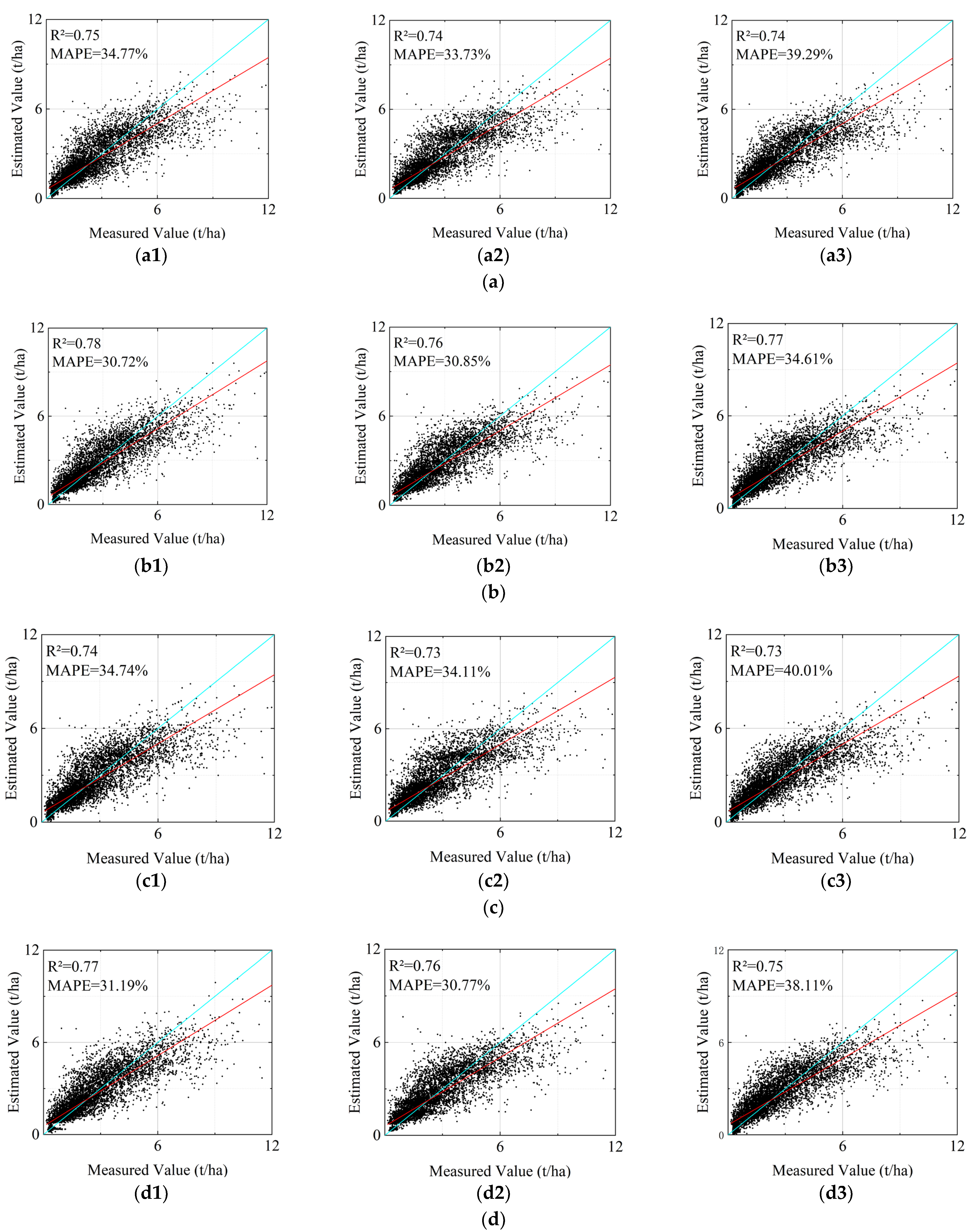
3.2.1. Evaluation of Data Schemes A and B

Data scheme B, which incorporates four additional categories of features, demonstrates a notable enhancement in performance metrics over scheme A. The coefficient of determination (R²) increased by 2.71%–4.40%. Concurrently, the MSE, RMSE, MAE, rRMSE, and MAPE all experienced reductions, with decreases spanning from 7.58% to 12.93%, 3.00% to 7.07%, 4.84% to 8.15%, 3.87% to 6.70%, and 8.55% to 11.9%, respectively. The comparative analysis of these metrics indicates that the LightGBM algorithm excels in predicting FCS. Specifically, when utilizing data scheme A, the LightGBM model demonstrated an R² of 0.75, alongside a MAPE of 34.77%. In contrast, employing data scheme B led to an improved R² of 0.78 and a reduced MAPE of 30.72%.

3.2.2. Evaluation of Data Schemes C and D

Similarly, data scheme D exhibited a marked enhancement in performance metrics compared to scheme C. The R² value increased by 2.99% to 4.05%, while MSE, RMSE, MAE, rRMSE, and MAPE saw decreases ranging from 8.23% to 11.60%, 3.96% to 6.00%, 5.13% to 7.19%, 4.20% to 5.98%, and 4.73% to 10.23%, respectively. The metrics indicate that the LightGBM algorithm continues to be the top performer in FCS prediction. For the LightGBM model, data scheme C yielded an R² of 0.74 and a MAPE of 34.74%. However, with data scheme D, the R² improved to 0.77, and the MAPE was reduced to 31.19%.

When comparing scheme B to scheme D, scheme B outperforms scheme D slightly in terms of R², MSE, RMSE, MAE, MAPE, and rRMSE. Specifically, the LightGBM model in scheme B achieves an R² of 0.78, a MSE of 0.85, an RMSE of 0.92, a MAE of 0.58, an rRMSE of 41.37%, and a MAPE of 30.72%. Scheme D yields an R² of 0.77, a MSE of 0.88, an RMSE of 0.94, a MAE of 0.59, an rRMSE of 42.11%, and a MAPE of 31.19%, demonstrating a solid performance. Scheme B incorporates more features (40), enabling it to capture greater data variability, which enhances the model’s predictive accuracy. The robust regularization capabilities of LightGBM allow scheme B to maintain a strong generalization performance. Figure 4 visually compares the performance indicators for the LightGBM, RF, and XGBoost models across different data schemes, further confirming LightGBM as the superior model for estimating FCS.

Figure 5 provides a detailed scatter plot illustrating the measured and estimated carbon stock values for the forest sub-compartments, as produced by the models (XGBoost, RF, and LightGBM), across four data schemes. The analysis reveals that data schemes incorporating ecological information features (B and D) exhibit superior performance, as evidenced by higher R² values and lower MAPE, compared to schemes without these features (A and C). The scatter plot demonstrates that the points generated by the LightGBM model are more closely aligned with the 1:1 line (the line extending from the bottom left to the top right), suggesting that the LightGBM model provides more accurate estimates of FCS than the RF and XGBoost models.

4. Discussion

4.1. Main Findings and Comparison with Previous Research

The study yields the following key conclusions: (1) Compared to the Lasso method, the RFE retains more feature information, thereby preserving the model’s performance and enhancing its generalization capability. (2) The LightGBM model outperforms both XGBoost and RF in terms of estimating FCS. (3) Incorporating ecological information features markedly improves the performance of the estimation models.

The performance indicators R² and rRMSE (%) are critical metrics in assessing the alignment between measured and estimated values. R² quantifies the model’s explanatory power, while rRMSE (%) determines the relative error between the model’s estimates and the measured values. Both metrics capture the proportional relationship between measured and estimated data rather than absolute discrepancies, rendering them independent from the sample data’s units of measurement. Consequently, this research benchmarks its R² and rRMSE (%) results against those reported in the literature, as detailed in

Table 7. Comparative analysis with previous research.

Scheme	Geran Wei [61]	Chenrui He [62]	Weimin Zou [63]	Our Study
R2	0.40	0.69	0.71	0.78
rRMSE (%)	47.44%	21.49%	-	41.37%

.

Table 7 shows that the R² performance index in this study has significantly improved compared to previous studies. Additionally, the rRMSE value remains commendably low, better than that in Geran Wei’s study (July 2024) but falling short of Chenrui He’s study (March 2024). Notably, Chenrui He’s research utilized only 1000 samples, a substantially smaller dataset, whereas our study employed 36,187 samples, incorporating a higher degree of noise. This suggests that the carbon stock model established by LightGBM in this study exhibits stronger explanatory power. The R² value achieved in this study is 0.78, exceeding the 0.71 reported by Weimin Zou (August 2023). Moreover, the research area of this study covers 168,267 ha, broader than the 101,199 ha in Weimin Zou’s study. This indicates the LightGBM algorithm has high accuracy and generalization ability in FCS estimation, delivering superior results even with an enlarged dataset and expanded study area.

4.2. Strengths and Limitations of This Study

A diverse range of data sources was used in this study, such as optical remote sensing data from S2 and L8 and radar remote sensing data from S1, along with DEM and FMP. An initial variable set was established, integrating spectral information from S2; textural features from S1 polarimetric signatures; terrain characteristics from DEM (such as elevation, slope, and aspect); and ground-based factors from FMP. By incorporating ecological information features and applying feature selection methods (RFE or Lasso), four data schemes were designed. Afterward, the XGBoost, LightGBM, and RF models were applied. This study makes the following primary contributions:

(1)

In the feature selection process, although the models built using Lasso and recursive feature elimination (RFE) methods show no significant difference in accuracy, the features selected by the two methods differ substantially. Lasso regression achieves feature selection and compression through L1 regularization. The selected features generally exhibit a relatively balanced importance, with most coming from remote sensing data. This suggests that, when forest background information is limited, the model constructed using Lasso feature selection can better leverage the information in remote sensing data, providing a more robust prediction performance. In contrast, the RFE method typically results in a more unbalanced distribution of feature importance by recursively evaluating features. During the RFE selection process, features related to forest background information are often assigned higher importance. This suggests that, in situations with abundant background information, especially those containing more forest-related features, the features selected by the RFE method better reflect the data’s underlying structure, enhancing the model’s adaptability. Although the differences in features selected by the two methods did not result in significant performance disparities, their differing feature selections define their respective applicable scenarios. The Lasso method is more suitable for situations dominated by remote sensing data and limited background information, while the RFE method performs better in scenarios with abundant background information, particularly when forest-related features dominate. Therefore, the selection of an appropriate feature selection method should depend on specific application requirements and data characteristics to maximize the model’s predictive ability and scope of application.

(2)

The inclusion of four ecological information features —namely, “community type”, “primary tree species”, “slope aspect”, and “humus thickness”—significantly improved model performance. These ecological information features enriched the model’s ecological background information and detailed microenvironmental data, improving its ability to describe soil–vegetation interactions. Specifically, information on “community type” and “primary tree species” enabled the model to assess vegetation adaptability to the environment, “slope aspect” influenced the microclimate factors, and “humus thickness” was correlated with soil fertility and water retention capacity. These variables optimized the model’s ability to capture complex ecological relationships, thereby enhancing prediction accuracy and generalization. Compared to scheme A without ecological information features, scheme B with ecological information features demonstrated significant improvement in model performance, with the R² increasing by 2.70%–4.00% and MSE, RMSE, MAE, rRMSE, and MAPE decreasing by 7.92%–12.37%, 3.00%–7.07%, 4.76%–7.94%, 3.87%–6.70%, and 8.54%–11.91%, respectively. These error indicators improve with the inclusion of features, indicating that the model performs better with additional input variables.

(3)

LightGBM improves the feature splitting efficiency significantly through a histogram-based bucketing algorithm and leaf growth strategy, enabling the effective processing of large-scale, high-dimensional data via parallelization and memory optimization. LightGBM’s native support for ecological information features eliminates the computational burden of one-hot encoding, further improving the resource utilization efficiency. Additionally, LightGBM offers a range of regularization parameters that effectively control model complexity and prevent overfitting, ensuring robust generalization capabilities and maintaining computational speed. These features position LightGBM as a superior choice over RF and XGBoost in various performance metrics. Under scheme B, the LightGBM model attained the following performance metrics: R² = 0.78, MSE = 0.85 t/ha, RMSE = 0.92, MAE = 0.58 t/ha, rRMSE = 41.37%, and MAPE = 30.72%, underscoring its high practical value and significance in FCS estimation.

(4)

Although the improvement in R² and error indices in this study is modest, these changes may still have a meaningful impact on practical applications, particularly in scenarios with large data volumes or high prediction accuracy requirements. Even a modest performance improvement may enhance the application value and prediction accuracy of the model in practical problems, such as carbon stock estimation, and holds practical significance for resource management and policymaking. Additionally, although the improvement in model performance from adding ecological information features is limited in this study area, considering the ecological and environmental differences across regions, more substantial improvements may be achieved in other study areas in the future. Therefore, future studies can further explore the potential of incorporating ecological features under different regional conditions, which may positively influence the accuracy of carbon stock models. In models with already high accuracy, small performance improvements are often more challenging; however, these improvements, although modest, reflect the subtle progress made by the algorithm in handling complex data. This modest improvement can be seen as a process of further adapting the model to the complexity of real-world data. Although the improvement is limited, it still demonstrates the potential for model optimization.

In contrast to previous studies, this study not only integrates multi-source remote sensing data but also combines ecological information (such as forest composition and main tree species) and environmental factors (such as humus depth and slope direction) to improve model accuracy and explores the use of the LightGBM model to estimate FCS over large areas. As a result of the limitations inherent in the experiment, there is a need for further optimization and refinement in the following areas:

(1)

Although this study demonstrates that the model performs well in Qingyuan County, its applicability remains limited. First, this study is based solely on the forest types and climate conditions of Qingyuan County and does not assess the model’s performance in other regions. As a result, it is unclear whether the model can perform similarly in regions with differing forest types, climate conditions, and ecological environments. In the future, as more regional data become available, it will be essential to further validate and refine the model to ensure its adaptability and generalization ability.

(2)

The accuracy of FCS estimation can be significantly improved by utilizing texture features derived from remote sensing images. In this study, texture features were only extracted from radar remote sensing images, and the exploration of different window sizes or asynchronous lengths was not undertaken. Exploring different window sizes, asynchronous lengths, and multiple band combinations to extract texture features from both optical and radar remote sensing images may offer valuable insights into how texture features enhance carbon stock estimation accuracy [64].

(3)

The remote sensing images analyzed in this study were largely captured in November and December, which may not coincide with the period of active tree growth. In autumn and winter, certain tree species may enter a dormant state, displaying yellowing or leaf fall. Consequently, the vegetation information captured, especially by optical imagery, might not accurately reflect the actual state of the trees, leading to potentially diminishing the model’s estimation accuracy. The acquisition of remote sensing images that align with the tree growth period in the future could lead to enhanced estimation accuracy [65].

(4)

This study relies on remote sensing images from just one temporal phase. Access to multi-temporal remote sensing data would enhance the model’s temporal and spatial resolution, as well as its estimation accuracy, by capturing seasonal and interannual dynamics of vegetation and its response to disturbances such as fire, pests, diseases, and logging. Such data would not only facilitate a detailed characterization of the spatiotemporal variability of carbon stock but also reveal long-term trends in carbon stock and its sensitivity to climate and land use changes, thereby providing a robust scientific foundation for carbon cycle research and climate policy formulation [66].

(5)

The accuracy in classification was a key factor in this study when forest composition, primary tree species, humus thickness, and slope aspect were applied as classification features for FCS estimation. The classification method chosen has a direct impact on the estimation of forest types and tree species distribution, which, in turn, affects the calculation of carbon stocks. If the classification method is inaccurate, it may lead to incorrect classification of forest types, resulting in the overestimation or underestimation of carbon stocks. For example, if the tree species or forest composition in certain areas are incorrectly classified, it may affect the regional distribution of carbon stocks, thereby influencing the overall carbon stock estimation.

(6)

In this study, we applied standard atmospheric correction methods tailored to each satellite data: Sen2Cor for Sentinel-2 (S2) and LaSRC for Landsat 8 (L8). However, the use of different correction methods may lead to differences in surface reflectivity, thus affecting the accuracy of carbon stock estimates. We plan to explore a unified atmospheric correction method or conduct more comparative experiments in future studies to improve the consistency and accuracy of the results.

5. Conclusions

This study utilized optical and radar remote sensing data, DEM, and FMP, applying three ML algorithms to estimate FCS across 36,187 forest sub-compartments in Qingyuan County. The key findings are summarized as follows:

(1)

The integration of ecological information features, such as forest composition, primary tree species, humus thickness, and slope direction, into the model significantly enhances the estimation accuracy and notably improves the overall model performance.

(2)

By retaining key features, the RFE algorithm efficiently reduces the number of independent variables, which accelerates the model training and boosts its generalization ability.

(3)

Among the three models—XGBoost, RF, and LightGBM—the LightGBM algorithm exhibits superior performance in estimating FCS.

Remote sensing technology and associated models offer valuable tools for large-scale soil carbon sequestration estimates, but their application in complex ecosystems, such as dense forests, remains constrained. The resolution of remote sensing data and sensor accuracy restrict accurate estimation of the soil carbon content in such areas. Moreover, factors like soil type, plant growth, and climate change introduce considerable variability, complicating precise predictions. While equation models offer theoretical insights, the complexity of forest ecosystems results in significant uncertainty. Thus, remote sensing and models are better suited as preliminary estimation tools, not definitive measurement methods.

Future research may enhance assessment precision by integrating remote sensing with field surveys and more accurate climate data. Additionally, refining algorithms and utilizing high-resolution data could improve model reliability, providing a more robust foundation for understanding carbon dynamics in dense forests and advancing carbon management strategies.

References

1. International Energy Agency. Net Zero by 2050. 2021. Available online: https://www.iea.org/reports/net-zero-by-2050 (accessed on 5 October 2024).
2. Sepehriar, A.; Eslamipoor, R. An Economical Single-Vendor Single-Buyer Framework for Carbon Emission Policies. J. Bus. Econ. 2024, 94, 927–945. [Google Scholar] [CrossRef]
3. Eslamipoor, R.; Sepehriar, A. Enhancing Supply Chain Relationships in the Circular Economy: Strategies for a Green Centralized Supply Chain with Deteriorating Products. J. Environ. Manag. 2024, 367, 121738. [Google Scholar] [CrossRef]
4. Pregitzer, K.S.; Euskirchen, E.S. Carbon Cycling and Storage in World Forests: Biome Patterns Related to Forest Age. Glob. Change Biol. 2004, 10, 2052–2077. [Google Scholar] [CrossRef]
5. Malhi, Y.; Meir, P.; Brown, S. Forests, Carbon and Global Climate. Philos. Trans. R. Soc. Lond. Ser. Math. Phys. Eng. Sci. 2002, 360, 1567–1591. [Google Scholar] [CrossRef]
6. Bustamante, M.M.C.; Roitman, I.; Aide, T.M.; Alencar, A.; Anderson, L.O.; Aragão, L.; Asner, G.P.; Barlow, J.; Berenguer, E.; Chambers, J.; et al. Toward an Integrated Monitoring Framework to Assess the Effects of Tropical Forest Degradation and Recovery on Carbon Stocks and Biodiversity. Glob. Change Biol. 2016, 22, 92–109. [Google Scholar] [CrossRef]
7. Pan, Y.; Birdsey, R.A.; Fang, J.; Houghton, R.; Kauppi, P.E.; Kurz, W.A.; Phillips, O.L.; Shvidenko, A.; Lewis, S.L.; Canadell, J.G.; et al. A Large and Persistent Carbon Sink in the World’s Forests. Science 2011, 333, 988–993. [Google Scholar] [CrossRef] [PubMed]
8. Chave, J.; Andalo, C.; Brown, S.; Cairns, M.A.; Chambers, J.Q.; Eamus, D.; Fölster, H.; Fromard, F.; Higuchi, N.; Kira, T.; et al. Tree Allometry and Improved Estimation of Carbon Stocks and Balance in Tropical Forests. Oecologia 2005, 145, 87–99. [Google Scholar] [CrossRef]
9. Santoro, M.; Cartus, O.; Carvalhais, N.; Rozendaal, D.M.A.; Avitabile, V.; Araza, A.; de Bruin, S.; Herold, M.; Quegan, S.; Rodríguez-Veiga, P.; et al. The Global Forest Above-Ground Biomass Pool for 2010 Estimated from High-Resolution Satellite Observations. Earth Syst. Sci. Data 2021, 13, 3927–3950. [Google Scholar] [CrossRef]
10. Harris, N.L.; Gibbs, D.A.; Baccini, A.; Birdsey, R.A.; de Bruin, S.; Farina, M.; Fatoyinbo, L.; Hansen, M.C.; Herold, M.; Houghton, R.A.; et al. Global Maps of Twenty-First Century Forest Carbon Fluxes. Nat. Clim. Change 2021, 11, 234–240. [Google Scholar] [CrossRef]
11. Dube, T.; Mutanga, O. Investigating the Robustness of the New Landsat-8 Operational Land Imager Derived Texture Metrics in Estimating Plantation Forest Aboveground Biomass in Resource Constrained Areas. ISPRS J. Photogramm. Remote Sens. 2015, 108, 12–32. [Google Scholar] [CrossRef]
12. Thenkabail, P.S.; Smith, R.B.; De Pauw, E. Hyperspectral Vegetation Indices and Their Relationships with Agricultural Crop Characteristics. Remote Sens. Environ. 2000, 71, 158–182. [Google Scholar] [CrossRef]
13. Vorovencii, I. Assessing Various Scenarios of Multitemporal Sentinel-2 Imagery, Topographic Data, Texture Features, and Machine Learning Algorithms for Tree Species Identification. IEEE J. Sel. Top. Appl. Earth Obs. Remote Sens. 2024, 17, 15373–15392. [Google Scholar] [CrossRef]
14. Whitcraft, A.K.; Vermote, E.F.; Becker-Reshef, I.; Justice, C.O. Cloud Cover throughout the Agricultural Growing Season: Impacts on Passive Optical Earth Observations. Remote Sens. Environ. 2015, 156, 438–447. [Google Scholar] [CrossRef]
15. Hirschmugl, M.; Deutscher, J.; Sobe, C.; Bouvet, A.; Mermoz, S.; Schardt, M. Use of SAR and Optical Time Series for Tropical Forest Disturbance Mapping. Remote Sens. 2020, 12, 727. [Google Scholar] [CrossRef]
16. Vatandaşlar, C.; Abdikan, S. Carbon Stock Estimation by Dual-Polarized Synthetic Aperture Radar (SAR) and Forest Inventory Data in a Mediterranean Forest Landscape. J. For. Res. 2022, 33, 827–838. [Google Scholar] [CrossRef]
17. Zhang, F.; Tian, X.; Zhang, H.; Jiang, M. Estimation of Aboveground Carbon Density of Forests Using Deep Learning and Multisource Remote Sensing. Remote Sens. 2022, 14, 3022. [Google Scholar] [CrossRef]
18. Zhang, Y.; He, B.; Chen, R.; Zhang, H.; Fan, C.; Yin, J.; Li, Y. The Potential of Optical and SAR Time-Series Data for the Improvement of Aboveground Biomass Carbon Estimation in Southwestern China’s Evergreen Coniferous Forests. GIScience Remote Sens. 2024, 61, 2345438. [Google Scholar] [CrossRef]
19. David, R.M.; Rosser, N.J.; Donoghue, D.N.M. Improving above Ground Biomass Estimates of Southern Africa Dryland Forests by Combining Sentinel-1 SAR and Sentinel-2 Multispectral Imagery. Remote Sens. Environ. 2022, 282, 113232. [Google Scholar] [CrossRef]
20. Luo, Z.; Viscarra-Rossel, R.A.; Qian, T. Similar Importance of Edaphic and Climatic Factors for Controlling Soil Organic Carbon Stocks of the World. Biogeosciences 2021, 18, 2063–2073. [Google Scholar] [CrossRef]
21. Hofhansl, F.; Chacón-Madrigal, E.; Fuchslueger, L.; Jenking, D.; Morera-Beita, A.; Plutzar, C.; Silla, F.; Andersen, K.M.; Buchs, D.M.; Dullinger, S.; et al. Climatic and Edaphic Controls over Tropical Forest Diversity and Vegetation Carbon Storage. Sci. Rep. 2020, 10, 5066. [Google Scholar] [CrossRef]
22. Zhang, S.; Fang, Y.; Luo, Y.; Li, Y.; Ge, T.; Wang, Y.; Wang, H.; Yu, B.; Song, X.; Chen, J.; et al. Linking Soil Carbon Availability, Microbial Community Composition and Enzyme Activities to Organic Carbon Mineralization of a Bamboo Forest Soil Amended with Pyrogenic and Fresh Organic Matter. Sci. Total Environ. 2021, 801, 149717. [Google Scholar] [CrossRef] [PubMed]
23. Qin, Y.; Feng, Q.; Holden, N.M.; Cao, J. Variation in Soil Organic Carbon by Slope Aspect in the Middle of the Qilian Mountains in the Upper Heihe River Basin, China. CATENA 2016, 147, 308–314. [Google Scholar] [CrossRef]
24. Zhang, X.; Adamowski, J.F.; Liu, C.; Zhou, J.; Zhu, G.; Dong, X.; Cao, J.; Feng, Q. Which Slope Aspect and Gradient Provides the Best Afforestation-Driven Soil Carbon Sequestration on the China’s Loess Plateau? Ecol. Eng. 2020, 147, 105782. [Google Scholar] [CrossRef]
25. Poorter, L.; van der Sande, M.T.; Thompson, J.; Arets, E.J.M.M.; Alarcón, A.; Álvarez-Sánchez, J.; Ascarrunz, N.; Balvanera, P.; Barajas-Guzmán, G.; Boit, A.; et al. Diversity Enhances Carbon Storage in Tropical Forests. Glob. Ecol. Biogeogr. 2015, 24, 1314–1328. [Google Scholar] [CrossRef]
26. Vesterdal, L.; Clarke, N.; Sigurdsson, B.D.; Gundersen, P. Do Tree Species Influence Soil Carbon Stocks in Temperate and Boreal Forests? For. Ecol. Manag. 2013, 309, 4–18. [Google Scholar] [CrossRef]
27. Ma, S.-H.; Eziz, A.; Tian, D.; Yan, Z.-B.; Cai, Q.; Jiang, M.-W.; Ji, C.-J.; Fang, J.-Y. Size- and Age-Dependent Increases in Tree Stem Carbon Concentration: Implications for Forest Carbon Stock Estimations. J. Plant Ecol. 2020, 13, 233–240. [Google Scholar] [CrossRef]
28. Augusto, L.; Boča, A. Tree Functional Traits, Forest Biomass, and Tree Species Diversity Interact with Site Properties to Drive Forest Soil Carbon. Nat. Commun. 2022, 13, 1097. [Google Scholar] [CrossRef] [PubMed]
29. Pham, T.D.; Yokoya, N.; Nguyen, T.T.T.; Le, N.N.; Ha, N.T.; Xia, J.; Takeuchi, W.; Pham, T.D. Improvement of Mangrove Soil Carbon Stocks Estimation in North Vietnam Using Sentinel-2 Data and Machine Learning Approach. GIScience Remote Sens. 2021, 58, 68–87. [Google Scholar] [CrossRef]
30. Singh, C.; Karan, S.K.; Sardar, P.; Samadder, S.R. Remote Sensing-Based Biomass Estimation of Dry Deciduous Tropical Forest Using Machine Learning and Ensemble Analysis. J. Environ. Manag. 2022, 308, 114639. [Google Scholar] [CrossRef] [PubMed]
31. Chen, Q.; Zhou, W.; Shi, W. Estimation of Soil Organic Carbon Density on the Qinghai–Tibet Plateau Using a Machine Learning Model Driven by Multisource Remote Sensing. Remote Sens. 2024, 16, 3006. [Google Scholar] [CrossRef]
32. Bui, Q.-T.; Pham, Q.-T.; Pham, V.-M.; Tran, V.-T.; Nguyen, D.-H.; Nguyen, Q.-H.; Nguyen, H.-D.; Do, N.T.; Vu, V.-M. Hybrid Machine Learning Models for Aboveground Biomass Estimations. Ecol. Inform. 2024, 79, 102421. [Google Scholar] [CrossRef]
33. Huang, L.; Huang, Z.; Zhou, W.; Wu, S.; Li, X.; Mao, F.; Song, M.; Zhao, Y.; Lv, L.; Yu, J.; et al. Landsat-Based Spatiotemporal Estimation of Subtropical Forest Aboveground Carbon Storage Using Machine Learning Algorithms with Hyperparameter Tuning. Front. Plant Sci. 2024, 15, 1421567. [Google Scholar] [CrossRef] [PubMed]
34. Zhou, R.; Wu, D.; Fang, L.; Xu, A.; Lou, X. A Levenberg–Marquardt Backpropagation Neural Network for Predicting Forest Growing Stock Based on the Least-Squares Equation Fitting Parameters. Forests 2018, 9, 757. [Google Scholar] [CrossRef]
35. Basler, D.; Körner, C. Photoperiod and Temperature Responses of Bud Swelling and Bud Burst in Four Temperate Forest Tree Species. Tree Physiol. 2014, 34, 377–388. [Google Scholar] [CrossRef]
36. Bai, C.; Zhao, W.; Klisz, M.; Rossi, S.; Shen, W.; Guo, X. Growth Rate and Not Growing Season Explains the Increased Productivity of Masson Pine in Mixed Stands. Plants 2025, 14, 313. [Google Scholar] [CrossRef]
37. Malhi, R.K.M.; Anand, A.; Srivastava, P.K.; Chaudhary, S.K.; Pandey, M.K.; Behera, M.D.; Kumar, A.; Singh, P.; Sandhya Kiran, G. Synergistic Evaluation of Sentinel 1 and 2 for Biomass Estimation in a Tropical Forest of India. Adv. Space Res. 2022, 69, 1752–1767. [Google Scholar] [CrossRef]
38. State Forestry Administration of China. Guidelines on Carbon Accounting and Monitoring for Afforestation Project (LY/T 2253-2014); State Forestry Administration of China: Beijing, China, 2014.
39. Mouret, F.; Albughdadi, M.; Duthoit, S.; Kouamé, D.; Rieu, G.; Tourneret, J.-Y. Reconstruction of Sentinel-2 Derived Time Series Using Robust Gaussian Mixture Models—Application to the Detection of Anomalous Crop Development. Comput. Electron. Agric. 2022, 198, 106983. [Google Scholar] [CrossRef]
40. Zhang, L.; Shao, Z.; Liu, J.; Cheng, Q. Deep Learning Based Retrieval of Forest Aboveground Biomass from Combined LiDAR and Landsat 8 Data. Remote Sens. 2019, 11, 1459. [Google Scholar] [CrossRef]
41. Fang, G.; Xu, H.; Yang, S.-I.; Lou, X.; Fang, L. Synergistic Use of Sentinel-1, Sentinel-2, and Landsat 8 in Predicting Forest Variables. Ecol. Indic. 2023, 151, 110296. [Google Scholar] [CrossRef]
42. Zhou, R.; Wu, D.; Zhou, R.; Fang, L.; Zheng, X.; Lou, X. Estimation of DBH at Forest Stand Level Based on Multi-Parameters and Generalized Regression Neural Network. Forests 2019, 10, 778. [Google Scholar] [CrossRef]
43. Huete, A.R. A Soil-Adjusted Vegetation Index (SAVI). Remote Sens. Environ. 1988, 25, 295–309. [Google Scholar] [CrossRef]
44. Jordan, C.F. Derivation of Leaf-Area Index from Quality of Light on the Forest Floor. Ecology 1969, 50, 663–666. [Google Scholar] [CrossRef]
45. Goel, N.S.; Qin, W. Influences of Canopy Architecture on Relationships between Various Vegetation Indices and LAI and Fpar: A Computer Simulation. Remote Sens. Rev. 1994, 10, 309–347. [Google Scholar] [CrossRef]
46. Wang, Q.; Moreno-Martínez, Á.; Muñoz-Marí, J.; Campos-Taberner, M.; Camps-Valls, G. Estimation of Vegetation Traits with Kernel NDVI. ISPRS J. Photogramm. Remote Sens. 2023, 195, 408–417. [Google Scholar] [CrossRef]
47. Sims, D.A.; Gamon, J.A. Relationships between Leaf Pigment Content and Spectral Reflectance across a Wide Range of Species, Leaf Structures and Developmental Stages. Remote Sens. Environ. 2002, 81, 337–354. [Google Scholar] [CrossRef]
48. Hardisky, M.A.; Daiber, F.C.; Roman, C.T.; Klemas, V. Remote Sensing of Biomass and Annual Net Aerial Primary Productivity of a Salt Marsh. Remote Sens. Environ. 1984, 16, 91–106. [Google Scholar] [CrossRef]
49. Cao, R.; Feng, Y.; Liu, X.; Shen, M.; Zhou, J. Uncertainty of Vegetation Green-Up Date Estimated from Vegetation Indices Due to Snowmelt at Northern Middle and High Latitudes. Remote Sens. 2020, 12, 190. [Google Scholar] [CrossRef]
50. Xiao, Y.; Zhang, J.; Cui, T.; Gong, J.; Liu, R.; Chen, X.; Liang, X. Remote Sensing Estimation of the Biomass of Floating Ulva Prolifera and Analysis of the Main Factors Driving the Interannual Variability of the Biomass in the Yellow Sea. Mar. Pollut. Bull. 2019, 140, 330–340. [Google Scholar] [CrossRef]
51. Adamu, B.; Ibrahim, S.; Rasul, A.; Whanda, S.J.; Headboy, P.; Muhammed, I.; Maiha, I.A. Evaluating the Accuracy of Spectral Indices from Sentinel-2 Data for Estimating Forest Biomass in Urban Areas of the Tropical Savanna. Remote Sens. Appl. Soc. Environ. 2021, 22, 100484. [Google Scholar] [CrossRef]
52. Cao, L. Estimation of Forest Stock Volume in Yanqing District Based on Sentinel-2 Images; Beijing Forestry University: Beijing, China, 2019. [Google Scholar]
53. Gitelson, A.A.; Merzlyak, M.N. Remote Estimation of Chlorophyll Content in Higher Plant Leaves. Int. J. Remote Sens. 1997, 18, 2691–2697. [Google Scholar] [CrossRef]
54. He, Y.; Yin, H.; Chen, Y.; Xiang, R.; Zhang, Z.; Chen, H. Soil Salinity Estimation Based on Sentinel-1/2 Texture Features and Machine Learning. IEEE Sens. J. 2024, 24, 15302–15310. [Google Scholar] [CrossRef]
55. Georgopoulos, N.; Gitas, I.Z.; Stefanidou, A.; Korhonen, L.; Stavrakoudis, D. Estimation of Individual Tree Stem Biomass in an Uneven-Aged Structured Coniferous Forest Using Multispectral LiDAR Data. Remote Sens. 2021, 13, 4827. [Google Scholar] [CrossRef]
56. Dar, A.A.; Parthasarathy, N. Patterns and Drivers of Tree Carbon Stocks in Kashmir Himalayan Forests: Implications for Climate Change Mitigation. Ecol. Process. 2022, 11, 58. [Google Scholar] [CrossRef]
57. Dar, A.A.; Parthasarathy, N. Ecological Drivers of Soil Carbon in Kashmir Himalayan Forests: Application of Machine Learning Combined with Structural Equation Modelling. J. Environ. Manag. 2023, 330, 117147. [Google Scholar] [CrossRef] [PubMed]
58. Huang, J.; Wu, D.; Fang, L. Identification of sub-compartment forest type based on multi-source data and three-tier models. J. Nanjing For. Univ. (Nat. Sci. Ed.) 2022, 46, 69. [Google Scholar] [CrossRef]
59. Illarionova, S.; Tregubova, P.; Shukhratov, I.; Shadrin, D.; Efimov, A.; Burnaev, E. Advancing Forest Carbon Stocks’ Mapping Using a Hierarchical Approach with Machine Learning and Satellite Imagery. Sci. Rep. 2024, 14, 21032. [Google Scholar] [CrossRef]
60. Cook-Patton, S.C.; Leavitt, S.M.; Gibbs, D.; Harris, N.L.; Lister, K.; Anderson-Teixeira, K.J.; Briggs, R.D.; Chazdon, R.L.; Crowther, T.W.; Ellis, P.W.; et al. Mapping Carbon Accumulation Potential from Global Natural Forest Regrowth. Nature 2020, 585, 545–550. [Google Scholar] [CrossRef]
61. Wei, G.; Li, M.; Quan, Y.; Wang, B.; Liu, J.; Ming, L. Geographically Weighted Random Forest Approach to Predict Forest Carbon Storage by Remote Sensing in Heilongjiang. J. Cent. South Univ. Forestry Technol. 2024, 44, 64–76. [Google Scholar] [CrossRef]
62. He, C.-R.; Pang, L.-F.; Tan, B.-X.; Huang, Y.-F.; Sun, X.-X. Remote Sensing Based Monitoring of Forest Aboveground Carbon Storage in Beijing. J. Northwest Forestry Univ. 2024, 39, 162–170. [Google Scholar] [CrossRef]
63. Zou, W.; Chen, C.; Huang, L.; Song, M.; Li, X.; Du, H. Geographic Weighted Regression Model Combined with Remote Sensing for Estimating Forest Aboveground Carbon Storage of Songyang County. Forest Res. Manag. 2023, 28, 132–140. [Google Scholar]
64. Duan, M.; Zhang, X. Using Remote Sensing to Identify Soil Types Based on Multiscale Image Texture Features. Comput. Electron. Agric. 2021, 187, 106272. [Google Scholar] [CrossRef]
65. Shi, S.; Zhao, P.; Zhou, M.; Yang, X. Biomass and carbon storage of the secondary forest (Populus davidiana) at different stand growing stages in southern Daxinganling temperate zone. Ecol. Environ. 2012, 21, 428–433. [Google Scholar]
66. Dahhani, S.; Raji, M.; Bouslihim, Y. Synergistic Use of Multi-Temporal Radar and Optical Remote Sensing for Soil Organic Carbon Prediction. Remote Sens. 2024, 16, 1871. [Google Scholar] [CrossRef]
Figure 1. Administrative boundaries and DEM of the study area.
Forests 16 00420 g001
Figure 2. Distribution map of FCS per hectare based on forest sub-compartments.
Forests 16 00420 g002
Figure 3. The importance of the features within the data schemes.
Forests 16 00420 g003
Figure 4. Comparison of the performance metrics for the RF, XGBoost, and LightGBM models within the data schemes. The panels represent the (a) R2, (b) mean squared error (MSE), (c) mean absolute error (MAE), and (d) mean absolute percentage error (MAPE). The schemes are as follows: A-RFE (without ecological information features), B-RFE (with ecological information features), C-Lasso (without ecological information features), and D-Lasso (with ecological information features).
Forests 16 00420 g004
Figure 5. Scatter plot of the estimated and measured FCS values for the LightGBM, XGBoost, and RF models. (a) Using RFE without ecological information features: (a1) LightGBM, (a2) RF, and (a3) XGBoost. (b) Using RFE with ecological information features: (b1) LightGBM, (b2) RF, and (b3) XGBoost. (c) Using Lasso without ecological information features: (c1) LightGBM, (c2) RF, and (c3) XGBoost. (d) Using Lasso with ecological information features: (d1) LightGBM, (d2) RF, and (d3) XGBoost. The blue diagonal line in the figure represents the identity line, and the red line represents the regression line of the model.
Forests 16 00420 g005