Abstract
Aboveground biomass (AGB) serves as an important indicator for assessing the productivity of forest ecosystems and exploring the global carbon cycle. However, accurate estimation of forest AGB remains a significant challenge, especially when integrating multi-source remote sensing data, and the effects of different feature combinations for AGB estimation results are unclear. In this study, we proposed a method for estimating forest AGB by combining Gao Fen 7 (GF-7) stereo imagery with data from Sentinel-1 (S1), Sentinel-2 (S2), and the Advanced Land Observing Satellite digital elevation model (ALOS DEM), and field survey data. The continuous tree height (TH) feature was derived using GF-7 stereo imagery and the ALOS DEM. Spectral features were extracted from S1 and S2, and topographic features were extracted from the ALOS DEM. Using these features, 15 feature combinations were constructed. The recursive feature elimination (RFE) method was used to optimize each feature combination, which was then input into the extreme gradient boosting (XGBoost) model for AGB estimation. Different combinations of features used to estimate forest AGB were compared. The best model was selected for mapping AGB distribution at 30 m resolution. The outcomes showed that the forest AGB model was composed of 13 features, including TH, topographic, and spectral features extracted from S1 and S2 data. This model achieved the best prediction performance, with a determination coefficient (R2) of 0.71 and a root mean square error (RMSE) of 18.11 Mg/ha. TH was found to be the most important predictive feature, followed by S2 optical features, topographic features, and S1 radar features.
1. Introduction
AGB is a critical indicator to assess the carbon storage and productivity of forest ecosystems. It is important in the study of the global carbon cycle, climate change, and sustainable forest management [1,2]. However, it remains a major challenge in remote sensing to efficiently and accurately estimate forest AGB. Traditional methods often rely on field survey data or single-sensor data, such as data from optical, radar, or LiDAR sensors. However, these methods face limitations in large-scale estimations, including high time costs, limited spatial coverage, and data saturation issues inherent to certain sensors [3,4].
Recent advancements in stereo imaging technology allow for the direct extraction of continuous tree height (TH) data by generating a digital surface model (DSM) in combination with a digital elevation model (DEM). TH structural information has been shown to overcome the saturation issue in traditional optical remote sensing methods for AGB estimation [5,6]. As a reliable indicator of forest vertical structure, TH exhibits a nonlinear relationship with AGB and provides stable estimates, especially in high-biomass regions. Compared to traditional spaceborne LiDAR data, stereo imagery enables efficient estimation of continuous forest TH. For example, Liu et al. [7] used SRTM elevation data and ZY-3 stereo imagery to produce a continuous canopy height map at 30 m resolution. Recent studies have demonstrated the effectiveness of stereo imagery, such as ZY-3 and WorldView-2, in estimating continuous TH and forest AGB [8,9,10]. These studies collectively demonstrate the potential of stereo imagery in extracting forest geometric parameter features. China’s GF-7 satellite is the first sub-meter-resolution stereo mapping satellite, which further improves the accuracy of forest TH estimation by generating high-precision DSM with a spatial resolution of less than 1 m [11,12,13]. This makes GF-7 particularly suitable for capturing continuous TH in complex terrains and high-biomass regions. However, the stereo imagery alone does not fully reflect the 3D structure of the forest, and high-precision DEM data are also required. In addition, spectral information on the tree canopy is also lacking when estimating forest AGB.
Integrating TH and optical imagery can effectively utilize the strengths of different data for AGB estimation. Optical remote sensing data that have a high spatial resolution and are rich in spectral information can assess forest canopy health and improve the precision of AGB estimates [14]. In most previous studies, forest AGB was estimated based on combined optical images and TH extracted from spaceborne LiDAR. For example, ICESat-2 and S2 data were used to develop a stratified hybrid method for AGB estimation [15]. GEDI LiDAR combined with the Landsat time series produced annual AGB maps for Mozambique [16]. Shendryk et al. [17] used GEDI, Sentinel-1 (S1), Sentinel-2 (S2), and elevation data to predict biomass at 100 m and 200 m resolution in Australia and the US. However, spaceborne LiDAR is susceptible to terrain slopes, resulting in inaccurate extracted forest vertical structure. Therefore, it is necessary to use stereo imagery. Li et al. [18] used ZY-3 stereo imagery and DEM data to derive continuous TH, combined with optical imagery, to estimate AGB in northern China’s coniferous forests. Puliti et al. [10] combined stereo-derived DSMs and high-quality DTMs to create CHMs, integrating them with S2 data to estimate AGB in Norway’s boreal forest using a random forest algorithm. Li et al. [18] used seasonal ZY-3 stereo imagery to derive relative canopy height, combining it with spectral data to estimate AGB in northern China’s larch plantations. These studies show that combining optical data with satellite-based stereo imagery is effective for large-scale forest AGB mapping.
At the same time, radar data have a unique advantage because of its all-weather capability and high-frequency observation, especially in cloud-covered areas. The use of synthetic aperture radar (SAR) data for forest AGB estimation has now become widely adopted. Lucas et al. [19] found that L-band SAR was better at capturing forest structure in high-biomass areas, while C-band was suitable for low- and medium-biomass areas. Furthermore, SAR data with various polarization modes enhanced the accuracy of AGB estimation. Li et al. [20] found that VV polarization was more sensitive for AGB estimation, while VH polarization better captured canopy details. Combining SAR data with optical data can fully utilize their complementary advantages and significantly enhance estimation accuracy. For example, Forkuor et al. [21] utilized S1 and S2 time series data, along with backscatter, spectral reflectance, and their derived features, to generate AGB maps for the Sudan region. Similarly, David et al. [22] achieved high-precision AGB estimation in Africa’s dry forests by integrating optical red-edge bands with SAR backscatter to reduce saturation effects in high-biomass areas. In addition to optical and SAR data as effective complementary factors, topographic variables such as elevation, slope, aspect, and the topographic wetness index (TWI) have been widely utilized in AGB estimation studies. These topographic factors can explain the spatial heterogeneity of the AGB and thus greatly improve the estimation accuracy. Liu et al. [23] combined topographic data with S1 radar and S2 optical data to estimate TH and biomass in northeast China. Xu et al. [24] demonstrated that the precision of forest AGB estimation was influenced by the topographic wetness index (TWI), terrain ruggedness, tree density, and wood proportion.
Although the combination of multi-source remote sensing data improves the assessment of AGB, its high-dimensional features increase modeling complexity and challenge practical applications [25,26]. The synergistic effects of multi-source remote sensing data are still poorly understood, and further research is needed to better improve the precision of forest AGB estimation [27,28]. To solve the problem mentioned above, this study aimed to develop an AGB estimation model based on the XGBoost method and to evaluate the contribution of different feature combinations of multi-source remote sensing data to AGB assessment. The specific studies include (1) integrating GF-7 stereo images and the Land Observing Satellite digital elevation model (ALOS DEM) to generate spatially continuous TH; (2) extracting spectral features of S1 and S2 and then combining the TH and ALOS DEM features to form 15 different feature combinations; (3) optimizing each feature combination using the RFE method and further comparing the contribution of each combination to the AGB estimation; and (4) generating a 30 m resolution AGB distribution map of the study area using the XGBoost model constructed with the selected optimal feature combinations.
2. Materials and Methods
2.1. Study Area
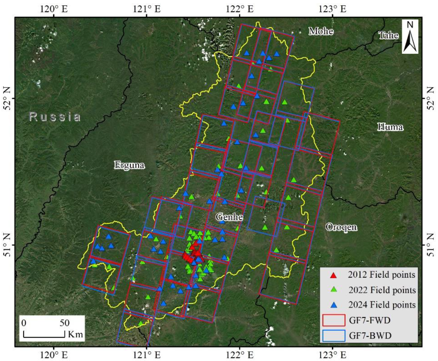
The research site is situated in Genhe City, northeastern China, covering an area of approximately 20,010 km2 (120.196–122.90° E, 50.414–52.517° N), as shown in Figure 1. It is within the Greater Khingan Mountains, extending broadly from northeast to southwest. Genhe primarily occupies the western slopes of the northern Greater Khingan Mountains, featuring a diverse landscape of low mountains and hills. The terrain gradually rises from 700 m in the southwest to 1300 m in the northeast, with an average elevation of 1000 m. The northern region is characterized by hilly plateaus, the central area consists of gentle slopes, and the southern part is characterized by steeper hills. Forests cover approximately 91.92% of the study area, spanning 1.84 million hectares, and constitute one of China’s most significant forest ecosystems and timber production bases. http://www.genhe.gov.cn/ (accessed on 8 November 2024). The forest composition is dominated by Dahurian larch (Larix gmelinii, Kuzen), which accounts for 82.77% of the total forest area, covering 1.14 million hectares. Other species, including white birch (Betula platyphylla, Sukaczev) and poplar (Populus davidiana, L.), are less abundant, collectively comprising approximately 290,000 hectares or 9.15% of the forested area [29].

Figure 1.
True-color image map of the study area. The red and blue lines show the spatial coverage of the forward and backward images of GF-7, respectively. The red, green, and blue triangular markers indicate the locations of the 2012, 2022, and 2024 sampling data, respectively.
2.2. Data Collection
2.2.1. Sampling Data
The field sampling was conducted three times in August 2012, February 2022, and August 2024, covering 53 plots (40 × 40 m), 83 plots (25 × 25 m), and 50 plots (25 × 25 m), respectively. A total of 186 plots were surveyed, 112 in coniferous forest and 74 in broadleaf forest, as shown in Figure 1. Sampling plots were evenly distributed across the study area, and factors such as forest type, topography, and elevation were carefully considered to ensure that the sample adequately represented the diversity of forest types and topographic variations within the study area. The field survey consisted of the following steps: the coordinates of the four corners and center point of each plot were accurately recorded using a Zenith 15R GPS RTK, and environmental parameters such as elevation, slope, and forest cover were recorded. In addition, measurements were taken for each tree in the sample plots, including tree height (TH), diameter at breast height (DBH), and height below branch for all trees with DBH > 5 cm. TH was calculated from distance and angle measurements, with distances being measured using a TruPulse 200 laser rangefinder, and angles being recorded using a Suunto PM-5/360PC mechanical goniometer.
To estimate the AGB of each sample plot, we used different allometric growth models depending on the dominant tree species in the plot, including larch, birch, and poplar, as shown in Table 1 [30]. The biomass of each tree was calculated by substituting the measured diameter at breast height (DBH) and tree height (TH) into the corresponding allometric growth model, whereas the total biomass of each sample plot was the sum of the biomass of all the trees within the plot. The calculations showed that the forest AGB values of the 186 sample plots ranged from 21.16 to 156.40 Mg/ha, with a mean value of 85.42 Mg/ha.

Table 1.
Allometric growth models for calculating the biomass of larch, birch, and poplar.
2.2.2. GF-7 Stereo Imagery Data
The GF-7 satellite, launched by China in 2019, represents the country’s first civilian satellite equipped with sub-meter-resolution stereo mapping capabilities. It is equipped with a dual-line camera (DLC) and is capable of obtaining stereo imagery with a backward resolution of 0.65 m and a forward resolution of 0.8 m. This advanced imaging capability enables the GF-7 to map and survey resources and generate high-resolution digital surface models (DSMs) that are critical for forest research. In this study, 37 GF-7 DLC images (Table S1) were utilized in combination with ALOS DEM data, which were accessed on 30 August 2010, to generate a continuous TH map of the study area. The DSMs derived from GF-7 were resampled to a resolution of 30 m to meet the scale requirements for forest AGB estimation.
2.2.3. Sentinel-2 Data
We obtained 11 S2 images from the Google Earth Engine (GEE) cloud platform. All images were acquired in October 2022, with cloud cover below 5% (Table S1). Images were selected in October to minimize cloud interference and retain essential spectral and biophysical information. In this study, we used four 10 m bands (490 nm, 560 nm, 665 nm, and 842 nm) and six 20 m bands, including three red-edge bands (705 nm, 740 nm, and 783 nm), one narrow NIR band (865 nm), and two shortwave infrared bands (1610 nm, 2190 nm). All bands were resampled using bilinear interpolation to a resolution of 30 m to ensure uniformity with other data resolutions.
In addition to spectral information, 24 commonly used vegetation indices were calculated based on processed S2 images [23,31]. Five biophysical variables were derived: leaf area index (LAI), fractional vegetation cover (FVC), leaf chlorophyll content (Cab), canopy water content (CWC), and fraction of absorbed PAR (FAPAR), as shown in Table 2 [23]. These spectral indices, vegetation indices, and biophysical characteristics effectively describe forest health and serve as inputs for forest AGB estimation models.
Table 2.
Description of predictor variables derived from remote sensing data for AGB estimation.
2.2.4. Sentinel-1 Data
In this study, we also used the S1 IW level products, which had high spatial and radiometric resolution and could capture backscatter intensity data widely used in AGB estimation [32,33]. S1 images offer dual polarization modes: vertically transmitted and vertically received (VV), and vertically transmitted and horizontally received (VH). These polarization patterns are very sensitive to forest characteristics such as canopy density and water content, and therefore they are also used as input parameters for AGB estimation models.
The S1 imagery was preprocessed to remove boundary and thermal noise, and then radiometric and topographic corrections were applied. Three radar-derived features were calculated from the processed S1 data (Table 2), which captured information related to forest structural properties [20]. To match the spatial resolution of the other datasets, features were resampled to 30 m using bilinear interpolation. To minimize the potential impacts of external factors such as rainfall and wind, we selected two S1 images acquired on 9 August 2021, from the GEE platform (Table S1).
2.2.5. Topographic Data
The ALOS DEM was generated from data acquired by PALSAR (phased array type L-band SAR), which is onboard the Advanced Land Observing Satellite (ALOS) and operated by the Japan Aerospace Exploration Agency (JAXA). PALSAR, utilizing L-band radar with a wavelength of approximately 15 cm, penetrates vegetation and cloud cover to acquire high-precision elevation data under diverse climatic and terrain conditions. In this study, ALOS DEM data were used to extract five topographic features: elevation, aspect, slope, slope position index (SPI), and topographic wetness index (TWI), as shown in Table 2. These features provide critical insights into terrain structure and moisture distribution, both of which significantly influence forest growth and AGB distribution [34]. Three ALOS DEM images covering the research area were acquired from the Alaska Satellite Facility https://search.asf.alaska.edu/ (accessed on 13 November 2024), all of which were acquired on 30 August 2010 and resampled to a resolution of 30 m to ensure compatibility with other datasets. Although the ALOS DEM data were acquired a time ago, there has been minimal change in topography during this time, making the ALOS DEM data suitable for this study.
2.3. Methods
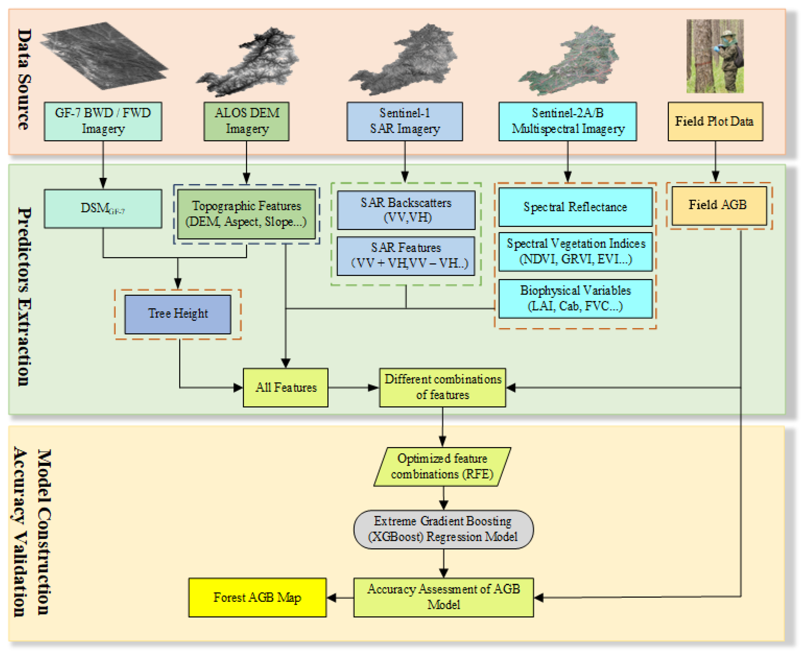
Most of the scientific literature does not explain in detail how different multi-source remote sensing features affect the estimation of forest AGB models. Based on this knowledge, we designed this experiment. We constructed 15 different combinations of remote sensing features, applied the RFE method to filter the features within each combination, and compared the precision of the optimized various feature combinations in estimating forest AGB. The experiments aim to scientifically identify the single variable optimal combinations so as to reveal the most suitable variable combinations. Finally, we used the XGBoost algorithm to estimate the forest AGB and generate a 30 m resolution forest AGB map. Figure 2 shows the flow of this experiment in detail.
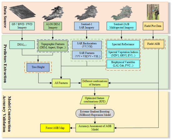
Figure 2.
Flowchart for the overall workflow of estimating forest AGB using combined multi-source remote sensing data.
2.3.1. Features Construction and Selection with RFE
The vertical structure of forests has been shown to significantly enhance forest AGB estimation accuracy. Although spaceborne LiDAR (e.g., GLAS, GEDI, and ICESAT2) is commonly used to acquire forest vertical structure, the results are typically discrete TH data that do not provide continuous TH information [15,35,36,37]. To address this limitation, continuous TH was estimated in this study using DSM generated from GF-7 stereo imagery in combination with ALOS DEM data, as shown in Equation (1).
where DSMGF-7 represents surface elevations from GF-7 stereo imagery, including vegetation and other surface features, and DEMALOS is the bare-earth elevation model obtained from ALOS.
The DSMs were extracted from the GF-7 stereo imagery using the OrthoEngine module of the Geomatica 2018 software (version SP1). The extraction process consisted of several steps. First, the forward and backward GF-7 images were relatively oriented using coplanarity equations and rational polynomial coefficients (RPCs) from the GF-7 metadata for accurate relative positioning. Second, 567 uniformly distributed ground control points (GCPs) were automatically extracted from Google reference images for horizontal coordinates, with elevations derived from the ALOS DEM to minimize fieldwork; points with errors exceeding 1 pixel were removed (Figure 3a). These GCPs ensured absolute orientation, including translation, rotation, and scaling. Third, 3250 tie points (TPs) were automatically collected between neighboring and forward/backward images, with erroneous points manually removed. These TPs were used to generate epipolar images, achieving an overall accuracy of 0.841 pixels (Figure 3b). Fourth, the DSM was evaluated using 100 reference points from Google images, with an average error of 0.384 m for both forward and backward images. Finally, the DSM was resampled to a 30 m resolution for subsequent analysis.
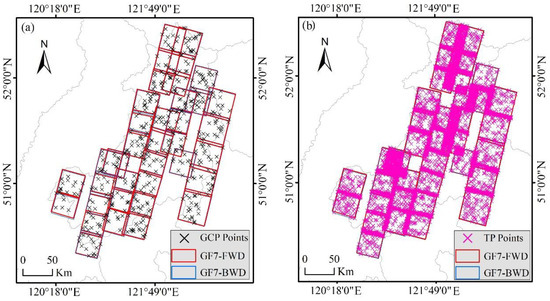
Figure 3.
Distribution of GCPs and TPs used for DSM generation. (a) Ground control points, (b) Tie points.
In addition to the TH feature, S1, S2, and ALOS DEM data and their derivatives were included in this study for estimating AGB (Table 2). Appropriate variables were initially selected based on previous studies, domain knowledge, and experience [26]. However, the variables required for biomass modeling varied across study areas due to differences in geographic and vegetation characteristics.
We used an RFE method to systematically reduce the feature set and identify the most relevant variables for modeling [38]. The feature selection process was implemented using the scikit-learn library (version 0.24) in Python (version 3.8). In the RFE process, we selected XGBoost (version 2.0) as the external estimator to assign weights to features and assess their relative importance. XGBoost evaluates feature importance by calculating the mean decrease in accuracy and the Gini importance during cross-validation, which helps in identifying the most important features for the model. The least important features were recursively removed from the current feature collection in each iteration, and the iterative procedure continued until the best subset of features was obtained. The performance of the selected feature subset was evaluated based on the coefficient of determination (R2) and root mean square error (RMSE) obtained from five-fold cross-validation.
2.3.2. Forest AGB Model with XGBoost
The XGBoost algorithm, with high robustness and ability to handle high-dimensional features, is widely used for forest structure parameter extraction and has played an important role in this field [22,39]. XGBoost was developed by Chen et al. [40] to achieve computational efficiency and superior performance by pushing boosted trees to their computational limits. In this study, the following hyperparameters of the XGBoost model were tuned to optimize performance: n_estimators was set to 500 to control the number of base learners (trees) in the model; the more trees, the greater the capacity of the model, but it may also lead to overfitting; max_depth was set to 6 to limit the maximum depth of each tree in order to balance the complexity and generalization of the model; learning_rate was set to 0.1 to control the optimization step size for each iteration, as a smaller learning rate helps to improve model stability; subsample was set to 0.8 and colsample_bytree was set to 0.8 to introduce stochasticity into the model training process and help to prevent overfitting by controlling the ratio of samples and features used; the gamma setting was 1.0 to control the minimum loss reduction required for further segmentation, making the model more conservative to avoid overfitting; and the regularization parameters lambda and alpha were set to 1.0 and 0.5, respectively, to add L2 (Ridge) and L1 (Lasso) regularization to prevent the model from becoming too complex. To reduce the time and memory consumption required to train the model, we used a heuristic search to iteratively tune these hyperparameters.
2.3.3. Accuracy Evaluation of Model
The field data were randomly categorized into 80% training set and 20% test set. We optimized as well as trained the predictive model utilizing the training dataset and tuned the hyperparameters. Subsequently, the accuracy and reliability of the models were assessed using the test dataset. The study used five-fold cross-validation to test the hyperparameters of the model and address potential overfitting issues. As model evaluation metrics, R2 and RMSE were applied to evaluate model performance. The model with the lowest RMSE and highest R2 was selected for the final AGB prediction.
where is the sample size, is the estimation of forest AGB, is the observation of forest AGB values, and is the mean of the observed AGB values.
3. Results
3.1. Feature Combination Comparison and Selection
In this study, a total of 15 feature combinations were composed, as shown in Table 3. Among them, the TH feature was derived from GF-7 stereo imagery and ALOS DEM data, while the other features were derived from S1, S2 and topographic data (DEM). Features were filtered using the RFE method, and the accuracy of different feature combinations was assessed by five-fold cross-validation. This approach assessed the estimation capabilities of different feature combinations and analyzed the change in model accuracy before and after performing RFE (Table 3). Bold boxes indicate datasets with the highest AGB estimation model accuracy in the same data combination category.
Table 3.
Test results of RFE selected features and various data combinations for AGB estimation.
For AGB estimation using a single data source, TH was the most precise, then S2 and topographic data, while S1 showed relatively poor performance. Among the two-source combinations, TH and S2 achieved the best results, followed by TH and topographic data. It is noteworthy that the combination of TH and S1 was significantly better than S1 alone. Combinations that lacked TH exhibited considerably lower accuracy, with S1 and DEM producing the poorest performance. For three-source combinations, TH, S2, and topographic data (TS2D) exhibited the highest estimation capability, whereas combinations without TH yielded the worst results. Finally, when all four data types (TS1S2D) were combined, the results showed that the model’s accuracy was very close to TS2D and was the highest among all data combinations. Overall, combining more data types generally led to improved estimation accuracy.
After applying the RFE method for feature filtering, we observed significant differences in the degree of feature selection and the number of features required for different data combinations. However, the model accuracy did not increase linearly with the number of features. Overall, after RFE filtering, the model accuracy of each feature combination improved to some extent, while the relative ranking of AGB estimation performance remained consistent. However, the TS1S2D and TS2D combinations consistently had the highest model accuracy. Notably, the R2 values for these two feature combinations were almost identical, indicating that the model predictions were most consistent and reliable with these feature combinations. This highlighted the robustness of the selected features and the effectiveness of RFE in determining the best set of features for AGB estimation.
3.2. AGB Model Validation and Feature Contribution Evaluation
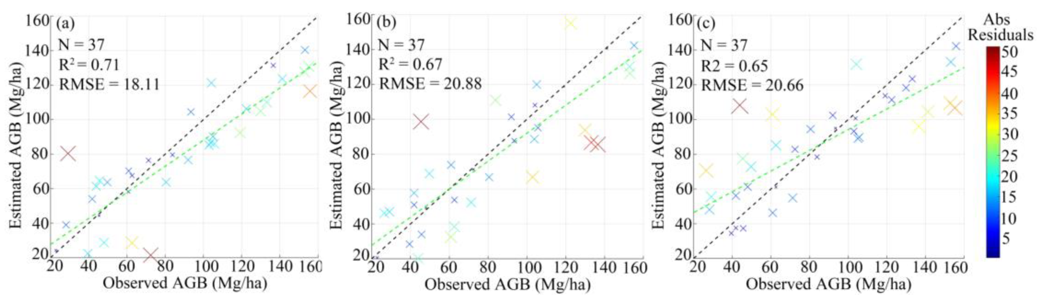
An XGBoost model was constructed using the filtered TS1S2D combination, and the hyperparameters of the model were optimized. Next, we evaluated the generalization ability of the final model using a test set and analyzed the performance of the two-feature combinations, TS2D and TS1S2, compared to TS1S2D. Figure 4a shows that the TS1S2D combination has the highest estimation accuracy with R2 = 0.71 and RMSE = 18.11 Mg/ha. The combination exhibits high correlation and low error in forest AGB estimation, indicating its ability to effectively capture the complex relationship between AGB and input features. Figure 4a also demonstrates that the residuals are mainly concentrated within 0 to 25 Mg/ha, with only two sample points having residuals above 40 Mg/ha. Based on the results of cross-validation and test set evaluation, the TS1S2D combination exhibited excellent generalization ability and was the best performer among the three-feature combinations.

Figure 4.
Performance of XGBoost models for AGB estimation using different feature combinations. (a) TS1S2D, (b) TS2D, (c) TS1S2.
In contrast, the TS2D combination in Figure 4b was slightly less accurate, with R2 = 0.67 and RMSE = 20.88 Mg/ha. Some samples of this combination showed large residuals in the prediction, with three sample points having residuals exceeding 40 Mg/ha and about five sample points within the range of 20–30 Mg/ha. Nonetheless, the TS2D combination also demonstrated good predictive ability and captured the AGB trend to some extent with acceptable errors. Although the TS2D and TS1S2D combinations achieved the same accuracy under RFE feature filtering, there were differences in their AGB estimation results.
Finally, the TS1S2 combination in Figure 4c performed relatively poorly, with the lowest precision, R2 = 0.65 and RMSE = 20.66 Mg/ha. Although only one sample point had absolute residuals greater than 40 Mg/ha, the residual colors are more dispersed than in the other combinations, suggesting greater prediction errors for many of the samples. This may have been due to the lack of DEM information in the TS1S2 combination, which limited the model’s ability to adequately capture the relationship between AGB and topographic correlates, thus reducing estimation accuracy. Overall, the TS1S2D combination performed the best in this study, with higher accuracy and stronger generalization ability, making it the most appropriate feature combination. Therefore, the XGBoost model with the TS1S2D combination was used for AGB prediction.
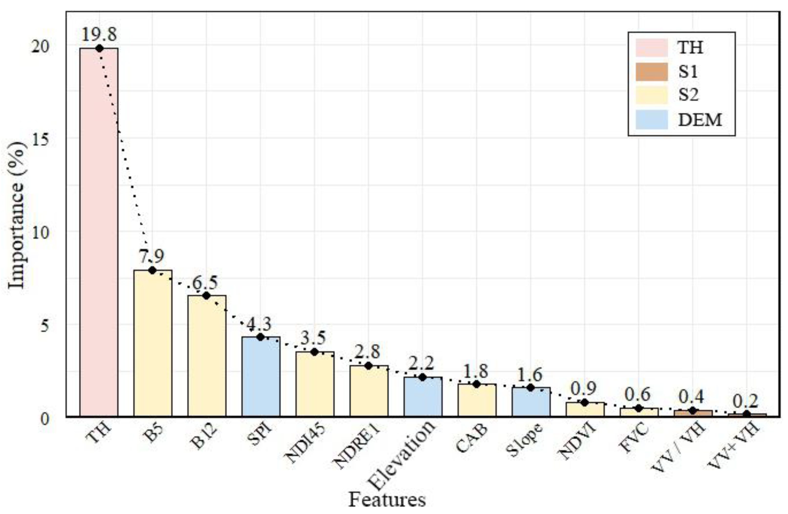
In addition, based on the importance analysis of TS1S2D features in the XGBoost model, Figure 5 demonstrates the proportion of the contribution of different predictors in forest AGB estimation. Among them, the TH feature had the largest contribution of 19.8%, indicating that the TH data are the key factor in the estimation model; followed by the B5 and B12 factors in the S2 optical data, with contribution rates of 7.9% and 6.5%, respectively, which reflects the dominant role of the optical remote sensing data in AGB estimation. Contribution from the topographic factor SPI reached 4.3%, while the contributions of the vegetation indices NDI45 and NDRE1 derived from S2 data were 3.5% and 2.8%, respectively, and were also influential. In contrast, the contribution of S1 data was low, with only 0.4% and 0.2% for VV/VH and VV + VH. These results suggest that TH data and S2 optical remote sensing data played a dominant role in AGB estimation in the study area, while the topographic factor SPI was also an important complement. In contrast, the two predictors of S1 were at the back of the contribution ranking and had a weak influence.
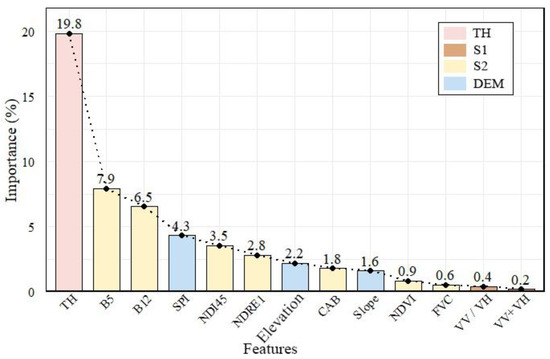
Figure 5.
Relative importance ranking of features based on the XGBoost model built with the TS1S2D feature combination.
3.3. Forest AGB Mapping
Figure 6a shows the spatial distribution of AGB estimated by the XGBoost model using the combination of TS1S2D. The AGB densities range from 18.0 Mg/ha to 181.2 Mg/ha in the study area. The predicted spatial distribution of AGB was consistent with Zhang et al. [41], i.e., the southwestern and central regions had lower AGB values, while the northern and southern regions had higher AGB values. Comparison with the S2 natural color composite map (Figure 6b) shows that the study results are in good agreement with the predicted AGB distribution (Figure 6c). The average AGB value for all pixels in the research area was 89.4 Mg/ha, which was very close to the observed average AGB value. Overall AGB in the research area was estimated to be 0.87 × 10⁸ Mg. Using a carbon transfer factor of 0.5, the overall carbon stock in the study area was calculated to be 0.43 × 10⁸ MgC.
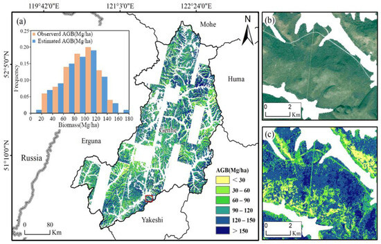
Figure 6.
Spatial distribution of AGB in the research area. (a) Distribution of AGB predicted by the XGBoost model with TS1S2D combination; (b) S2 true-color image of the region within the red box; (c) zoomed-in view of the red box in the AGB distribution map.
4. Discussion
4.1. Analysis of Feature Combinations of Multi-Source Data in Forest AGB Estimation
This study evaluated the effectiveness of the single TH feature and the features derived from S1, S2, and DEM data, as well as the effectiveness of their combinations. The RFE method was used to optimize each feature combination, and the results were assessed through five-fold cross-validation. Most studies have indicated that TH can directly reflect the vertical structure of forests and has played a crucial role in AGB estimation [42,43]. Table 3 of this study also shows that removing the TH feature significantly reduces the prediction accuracy of the model, especially in all combinations of two or three datasets. Therefore, the continuous-type TH generated using stereo imagery combined with topographic DEM can be used as an ideal input parameter for forest AGB. This method not only overcomes the limitations of spaceborne LiDAR data in sampling density and spatial coverage but also effectively corrects the slope effect by introducing terrain factors. However, the method depends highly on high-precision DEM data, and in the future, DEMs with higher precision will be generated using SAR data with longer wavelengths (e.g., P-band).
Among the two-data-source combinations, the TS2 combination showed the highest estimation accuracy (R2 = 0.48, RMSE = 24.26 Mg/ha), suggesting that combining TH with canopy spectral information was more effective in estimating forest AGB in this study. The contribution of topographic features was better than that of S1 data features among the three- or four-source combinations, which is shown in Figure 5. This discovery is different from the results of previous studies by Yang et al. [44] and Liu et al. [23]. This may be due to the fact that mountainous terrain features have a significant impact on AGB estimation. In addition, S1 is a C-band SAR data type, which is susceptible to the effects of vegetation canopy water content and soil wetness [45]. The S1 data used in this study were focused on the growing season, so these influences were even more pronounced. Previous studies have shown that shorter wavelength SAR (e.g., C band and X band) is more responsive to smaller canopy elements, whereas longer wavelength SAR (e.g., L band and P band) is more suitable for estimation of high-biomass areas due to its ability to better capture the structural information of tree branches and trunks [45,46,47,48,49]. Therefore, future studies should investigate more the possibility of longer-wavelength SAR data and assess their impact on improving the accuracy of AGB estimates when combined with other data.
A comparison of AGB estimation accuracies under different data combinations revealed that combining three types of data was significantly better than combinations of only two types. Among combinations of three types of data, TS2D had the highest precision of estimation with R2 = 0.60 and RMSE = 21.32 Mg/ha, which was almost the same as the combination containing four types of data (TS1S2D) (R2 = 0.60 and RMSE = 21.28 Mg/ha). However, the TS1S2D combination used only 13 features, while the TS2D combination used 16 features. This indicated that TS1S2D was able to achieve comparable accuracy to TS2D with fewer features. Table 4 lists the features selected for the two combinations, where different features are indicated in bold font. The analysis revealed that when S1 is unavailable, it can be supplemented by the B3, B11, CWC, and GNDVI features from the S2 data, along with the TWI features from the DEM data, achieving the same estimation accuracy as the TS1S2D combination. This suggests a high flexibility of data combinations in forest AGB estimation and some substitutability between different data types. It is worth noting that the two features, CWC and TWI, correlate closely with vegetation moisture content and soil moisture content, which have a strong influence on the backscattering coefficient of S1. Therefore, these two features were selected into the model in the TS2D combination. However, when the S1 data were introduced, these features were again dropped by the RFE filter, suggesting that the S1 data were able to directly characterize these influences, thus replacing the relevant features.
Table 4.
Comparison of feature selection results of TS2D and TS1S2D combinations.
4.2. Analysis of AGB Estimates for Different Forest Types
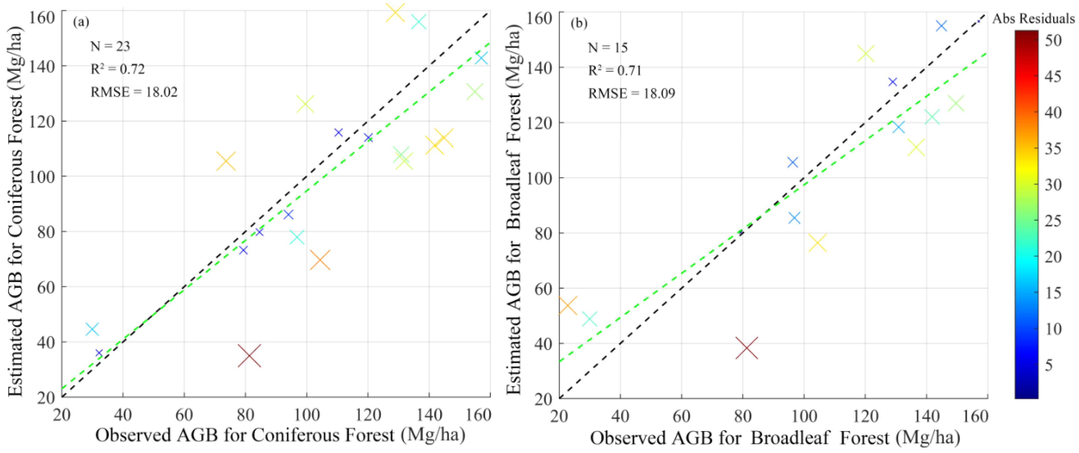
In order to explore the impact of different features in the TS1S2D combinations on the estimation of AGB in different forest types, the study used the XGBoost method and the combination of TS1S2D features to estimate the AGB in coniferous and broadleaf forests, respectively, as shown in Figure 7. The model had similar but slightly different estimation accuracies for coniferous forests (Figure 7a) and broadleaf forests (Figure 7b). The R2 value of 0.72 for the coniferous forest is slightly higher than that of 0.71 for the broadleaf forest, indicating that the model is more capable of assessing the coniferous forest. However, the RMSE values of 18.02 Mg/ha and 18.09 Mg/ha, respectively, indicate that the estimation errors are almost the same for both forest types. The reason for the similarity of the errors is that the same combination of features was used in estimating the two forest types.

Figure 7.
Forest AGB estimation based on XGBoost model and TS1S2D feature combination. (a) Coniferous forests, (b) Broadleaf forests.
Figure 7 shows that coniferous forests have residuals greater than 35 Mg/ha in the 80–140 Mg/ha range, while broadleaf forests have residuals greater than 35 Mg/ha in the 20–90 Mg/ha range. These differences suggest that model performance varies across forest types in different AGB ranges, which may be due to differences in structural characteristics (e.g., tree density and canopy structure) across forest types. Coniferous forests typically have a more uniform canopy structure and therefore show larger residuals in the medium to high AGB range. In contrast, broadleaf forests are more variable in canopy structure and leaf area index and therefore show larger residuals for estimates in the low to medium AGB range.
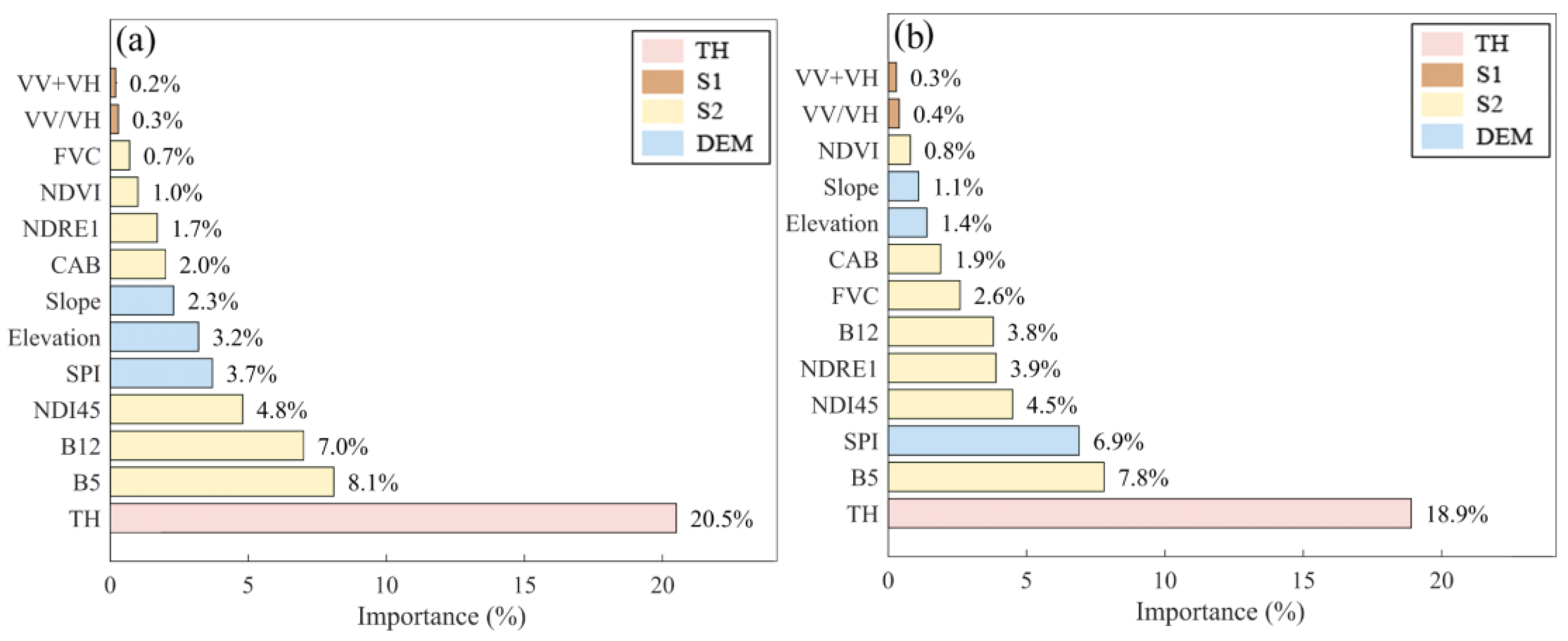
In addition, this study ranked the importance of features of the TS1S2D combination for different forest types. As shown in Figure 8, TH has the highest importance among all features, with 20.5% for coniferous forests (Figure 8a) and 18.9% for broadleaf forests (Figure 8b). In coniferous forests, the higher explanatory power of TH may be attributed to their relatively homogeneous structure, where TH serves as a reliable proxy for biomass. In contrast, although TH remains an important feature in broadleaf forests, the influence of TH may be reduced due to a more complex canopy structure where other features can play a greater role. Overall, TH is a central variable in AGB estimation. While previous studies primarily relied on LiDAR-derived TH [42,43,50], this study is the first to use continuous TH derived from stereo imagery and topographic data to estimate AGB in different forest types.
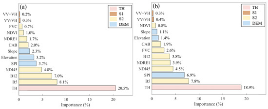
Figure 8.
Feature importance rankings for different forest types based on the XGBoost model and TS1S2D feature combination. (a) Coniferous forests, (b) Broadleaf forests.
In coniferous forests, the spectral features B5 and B12 were of great importance, which is in agreement with previous studies [51]. Because the canopy structure is more uniform and the spectral reflectance is more stable in coniferous forests, B5 and B12 can effectively capture canopy information. In broadleaf forests, although the importance of B5 is still high, the importance of B12 decreases significantly. This may be due to the complex canopy structure of broadleaf forests, where the reflectance properties of different leaves vary greatly, reducing the ability of a single band to interpret biomass.
The vegetation indices reflect the health of the canopy, and NDI45 shows a good performance in both forest types, as shown in Figure 8. However, in broadleaf forests in addition to the NDI45 feature, the NDRE1 feature also shows high importance, which was not found in previous studies. Overall, vegetation indices are more important in broadleaf forests, where NDI45 and NDRE1 are significantly more important in broadleaf forests than in coniferous forests. This may be due to the large canopy width of broadleaf forests, which allows vegetation indices to capture information more effectively.
The topographic features of coniferous forests are more important than those of broadleaf forests. In the study area, coniferous forests are widely distributed on mountains and slopes with complex topography, and topographic conditions have an important influence on the growth of coniferous forests. Elevation and slope, as a reflection of environmental conditions, are particularly important for the growth of coniferous forests. In contrast, broadleaf forests are mostly found in gently sloping areas, where elevation and slope are less important. However, the SPI feature is relatively more important in broadleaf forests, probably because broadleaf forests are usually located in wet, low-lying areas, where the strength of water flow and humidity have a greater influence on their growth. This discovery is also interesting. In coniferous forests, SPI also plays a role, but the effect is relatively small. Finally, the importance of VV/VH and VV + VH features is low in both forest types, probably because they offer limited information gain to significantly increase the precision of AGB estimates. The differences in the importance of these features ultimately led to differences in AGB estimation results between coniferous and broadleaf forests.
4.3. Comparative Analysis of AGB Estimation
The XGBoost model based on TS1S2D performed the best (R2 = 0.71, RMSE = 18.11 Mg/ha), and thus was selected as the final prediction model for the spatial distribution of whole-forest AGB in the research area, as shown in Figure 6. The model estimation results show that the average AGB value in the research area was 89.41 mg/ha, mainly concentrated within 70–150 mg/ha. This is related to the more than 80% forest cover in the research area. In addition, the XGBoost model was used in this study to predict the spatial AGB by combining two combinations of TS2D and TS1S2 (Figure S1), aiming to compare with the TS1S2D combination.
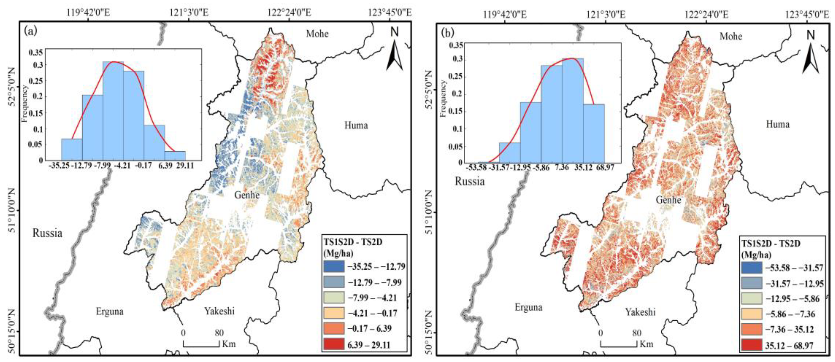
Difference maps were generated by subtracting the spatial prediction results of TS1S2D from those of TS2D and TS1S2, and the categorization of the difference maps was statistically analyzed (Figure 9). Although the estimation accuracy was similar for the three feature combinations, the spatial distribution of AGB was significantly different, as shown in Figure 9a. Especially in the central region, the TS2D estimate was significantly lower than the TS1S2D combination, while in the edge region it was again higher than the TS1S2D combination.

Figure 9.
AGB difference maps. (a) TS2D–TS1S2D, (b) TS1S2–TS1S2D.
The complex topography and high forest density may have led to significant differences in the adaptability of different feature combinations in these regions. In the central region, the influence of S1 data on AGB estimation was more pronounced, resulting in higher TS1S2D estimates than TS2D, whereas in edge areas with gentle terrain or less contribution from S1 data, the TS1S2D estimate was lower than TS2D. This positive and negative phenomenon may be due to the differential effect of S1 data on AGB estimation under different terrain conditions and vegetation structures. We suggest that future studies further explore the applicability of S1 data in different regions, especially the effect mechanism in areas with complex terrain or high forest density. As shown in Figure 9b, the AGB estimate for TS1S2 was generally higher than TS1S2D, which indicates an overestimation of TS1S2 in the absence of topographic data. This further emphasizes the importance of topographic data in AGB estimation, especially in regions with terrain complexity. The incorporation of topographic data can significantly reduce the bias of overestimation of AGB in high-elevation and steep-slope areas.
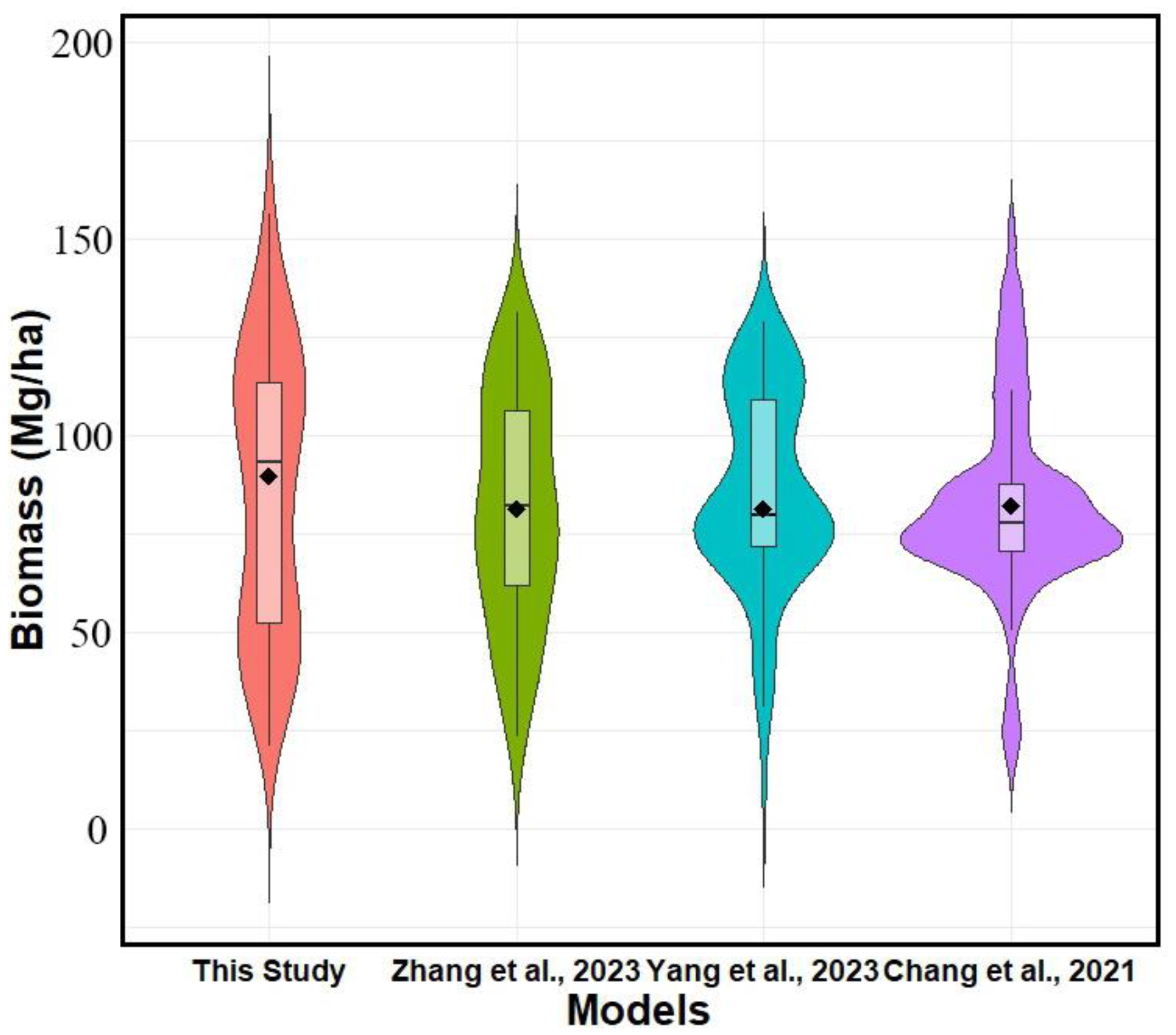
In addition, we compared the results of the study with AGB estimates from several published datasets covering the research area. Figure 10 shows the distribution of AGB from this study and three published datasets. The median AGB varies from 82.236 Mg/ha in Zhang et al. [41], 80.041 Mg/ha in Yang et al. [44], and 77.867 Mg/ha in Chang et al. [52] to the highest value of 90.145 Mg/ha in our study. Chang et al. [52] reported the lowest median, whereas our study demonstrates a relatively high range of AGB estimates and the highest median. This further suggests that our study can effectively eliminate saturation effects and estimate AGB across a wider range. The highest mean value estimated in this study was 89.41 Mg/ha, versus 81.729 Mg/ha in Yang et al. [44], 82.301 Mg/ha in Chang et al. [52], and 81.437 Mg/ha in Zhang et al. [41]. This also indicates that our approach can increase the precision of AGB estimation in high-density forest areas.
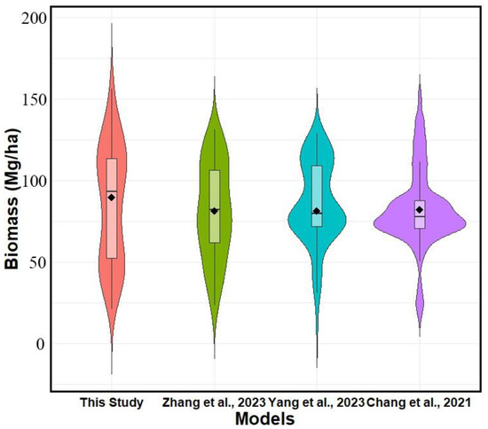
Figure 10.
Comparison of AGB distributions in this study and published datasets (Zhang et al. [41], Yang et al. [44], Chang et al. [52]). The horizontal line in each box plot represents the median, the black dot indicates the mean, and the width of the violin plot reflects the data proportion.
5. Conclusions
Accurate assessment of AGB on a global or regional scale is essential for forest conservation, management, and sustainable development. In this study, we successfully generated 30m resolution AGB maps of the Genhe region in China by integrating field data with GF-7 stereo imagery and S2, S1, and ALOS DEM data. The outcomes showed that the combination of TH features derived from GF-7 stereo imagery and the ALOS DEM with features from S1, S2, and DEM is the best model for AGB estimation. Among the predicted variables, TH was considered to be the most important, while B5 and B12 from S2 also contributed significantly to the accuracy of AGB estimation. Topographic features were also particularly important in AGB estimation, even more important than S1 data, especially in complex terrain. By using the XGBoost algorithm, this study achieved highly accurate AGB estimation, and the validation results confirmed the robustness of the model. This research further proves the importance of multi-source remote sensing data in AGB estimation, especially the potential of the combination of stereo imagery, optical data, and topographic data in improving the accuracy of AGB estimation. Future research should further explore how to maximize the use of existing data, develop more advanced machine learning models such as deep learning, and validate the applicability of data combinations in different regions and forest types to support a wider range of applications.
Supplementary Materials
The following supporting information can be downloaded at: https://www.mdpi.com/article/10.3390/f16020347/s1, Figure S1: Spatial distribution obtained from XGBoost model prediction based on TS1S2D (a), TS2D (b) and TS1S2 (c); Table S1: Image acquisition date and scene ID.
Author Contributions
D.W.: Conceptualization, Methodology, Software, Writing—original draft. Y.X.: Conceptualization, Resources, Funding acquisition. A.F.: Formal analysis, Writing—review & editing. J.T.: Formal analysis, Writing—review & editing. X.C.: Formal analysis, Writing—review & editing. H.Y.: Formal analysis, Writing—review & editing. S.Y.: Formal analysis, Writing—review & editing. Y.L.: Formal analysis, Writing—review & editing. All authors have read and agreed to the published version of the manuscript.
Funding
This work is supported by the National Key R&D Program of China (No. 2021YFE0117700) and the Program for Young Talents of Basic Research in Universities of Heilongjiang Province (No. YQJH2024004).
Data Availability Statement
Data will be made available on request.
Acknowledgments
The authors thank colleagues for field surveys and data collection. We appreciate the Institute of Forest Resource Information Techniques, CAF, for GF-7 stereo imagery, the Google Earth Engine for Sentinel data, and the Alaska Satellite Facility for ALOS DEM data.
Conflicts of Interest
The authors declare that they have no known competing financial interests or personal relationships that could have appeared to influence the work reported in this paper.
References
- Baccini, A.; Walker, W.; Carvalho, L.; Farina, M.; Sulla-Menashe, D.; Houghton, R.A. Tropical Forests Are a Net Carbon Source Based on Aboveground Measurements of Gain and Loss. Science 2017, 358, 230–234. [Google Scholar] [CrossRef] [PubMed]
- Qi, Z.; Li, S.; Pang, Y.; Zheng, G.; Kong, D.; Li, Z. Assessing Spatiotemporal Variations of Forest Carbon Density Using Bi-Temporal Discrete Aerial Laser Scanning Data in Chinese Boreal Forests. For. Ecosyst. 2023, 10, 100135. [Google Scholar] [CrossRef]
- Chave, J. Ground Data Are Essential for Biomass Remote Sensing Missions. Surv. Geophys. 2019, 40, 863–880. [Google Scholar] [CrossRef]
- Guo, R.; Gao, J.; Fu, S.; Xiu, Y.; Zhang, S.; Huang, X.; Feng, Q.; Liang, T. Estimating Aboveground Biomass of Alpine Grassland During the Wilting Period Using In Situ Hyperspectral, Sentinel-2, and Sentinel-1 Data. IEEE Trans. Geosci. Remote Sens. 2024, 62, 1–16. [Google Scholar] [CrossRef]
- Huang, R.; Yao, W.; Xu, Z.; Cao, L.; Shen, X. Information Fusion Approach for Biomass Estimation in a Plateau Mountainous Forest Using a Synergistic System Comprising UAS-Based Digital Camera and LiDAR. Comput. Electron. Agric. 2022, 202, 107420. [Google Scholar] [CrossRef]
- Tian, L.; Wu, X.; Tao, Y.; Li, M.; Qian, C.; Liao, L.; Fu, W. Review of Remote Sensing-Based Methods for Forest Aboveground Biomass Estimation: Progress, Challenges, and Prospects. Forests 2023, 14, 1086. [Google Scholar] [CrossRef]
- Liu, M.; Cao, C.; Dang, Y.; Ni, X. Mapping Forest Canopy Height in Mountainous Areas Using ZiYuan-3 Stereo Images and Landsat Data. Forests 2019, 10, 105. [Google Scholar] [CrossRef]
- Ni, W.; Yu, T.; Pang, Y.; Zhang, Z.; He, Y.; Li, Z.; Sun, G. Seasonal Effects on Aboveground Biomass Estimation in Mountainous Deciduous Forests Using ZY-3 Stereoscopic Imagery. Remote Sens. Environ. 2023, 289, 113520. [Google Scholar] [CrossRef]
- Persson, H.J.; Perko, R. Assessment of Boreal Forest Height from WorldView-2 Satellite Stereo Images. Remote Sens. Lett. 2016, 7, 1150–1159. [Google Scholar] [CrossRef]
- Puliti, S.; Hauglin, M.; Breidenbach, J.; Montesano, P.; Neigh, C.S.R.; Rahlf, J.; Solberg, S.; Klingenberg, T.F.; Astrup, R. Modelling Above-Ground Biomass Stock over Norway Using National Forest Inventory Data with ArcticDEM and Sentinel-2 Data. Remote Sens. Environ. 2020, 236, 111501. [Google Scholar] [CrossRef]
- Du, L.; Pang, Y.; Ni, W.; Liang, X.; Li, Z.; Suarez, J.; Wei, W. Forest Terrain and Canopy Height Estimation Using Stereo Images and Spaceborne LiDAR Data from GF-7 Satellite. Geo-Spat. Inf. Sci. 2023, 27, 811–821. [Google Scholar] [CrossRef]
- Li, G.; Gao, X.; Hu, F.; Guo, A.; Liu, Z.; Chen, J.; Liu, C.; Nie, S.; Fu, A. OVERVIEW OF THE TERRESTRIAL ECOSYSTEM CARBON MONITORING SATELLITE LASER ALTIMETER. Int. Arch. Photogramm. Remote Sens. Spat. Inf. Sci. 2022, XLIII-B1-2022, 53–58. [Google Scholar] [CrossRef]
- Sun, Z.; Li, P.; Wang, D.; Meng, Q.; Sun, Y.; Zhai, W. Recognizing Urban Functional Zones by GF-7 Satellite Stereo Imagery and POI Data. Appl. Sci. 2023, 13, 6300. [Google Scholar] [CrossRef]
- Li, H.; Hiroshima, T.; Li, X.; Hayashi, M.; Kato, T. High-Resolution Mapping of Forest Structure and Carbon Stock Using Multi-Source Remote Sensing Data in Japan. Remote Sens. Environ. 2024, 312, 114322. [Google Scholar] [CrossRef]
- Varvia, P.; Saarela, S.; Maltamo, M.; Packalen, P.; Gobakken, T.; Næsset, E.; Ståhl, G.; Korhonen, L. Estimation of Boreal Forest Biomass from ICESat-2 Data Using Hierarchical Hybrid Inference. Remote Sens. Environ. 2024, 311, 114249. [Google Scholar] [CrossRef]
- Liang Mengyu, M.; Duncanson, L.; Silva, J.A.; Sedano, F. Quantifying Aboveground Biomass Dynamics from Charcoal Degradation in Mozambique Using GEDI Lidar and Landsat. Remote Sens. Environ. 2023, 284, 113367. [Google Scholar] [CrossRef]
- Shendryk, Y. Fusing GEDI with Earth Observation Data for Large Area Aboveground Biomass Mapping. Int. J. Appl. Earth Obs. Geoinf. 2022, 115, 103108. [Google Scholar] [CrossRef]
- Li, G.; Xie, Z.; Jiang, X.; Lu, D.; Chen, E. Integration of ZiYuan-3 Multispectral and Stereo Data for Modeling Aboveground Biomass of Larch Plantations in North China. Remote Sens. 2019, 11, 2328. [Google Scholar] [CrossRef]
- Lucas, R.M.; Mitchell, A.L.; Armston, J. Measurement of Forest Above-Ground Biomass Using Active and Passive Remote Sensing at Large (Subnational to Global) Scales. Curr. For. Rep. 2015, 1, 162–177. [Google Scholar] [CrossRef]
- Li, J.; Bao, W.; Wang, X.; Song, Y.; Liao, T.; Xu, X.; Guo, M. Estimating Aboveground Biomass of Boreal Forests in Northern China Using Multiple Datasets. IEEE Trans. Geosci. Remote Sens. 2024, 62, 1–10. [Google Scholar] [CrossRef]
- Forkuor, G. Above-Ground Biomass Mapping in West African Dryland Forest Using Sentinel-1 and 2 Datasets—A Case Study. Remote Sens. Environ. 2020, 236, 111496. [Google Scholar] [CrossRef]
- David, R.M.; Rosser, N.J.; Donoghue, D.N.M. Improving above Ground Biomass Estimates of Southern Africa Dryland Forests by Combining Sentinel-1 SAR and Sentinel-2 Multispectral Imagery. Remote Sens. Environ. 2022, 282, 113232. [Google Scholar] [CrossRef]
- Liu, Y.; Gong, W.; Xing, Y.; Hu, X.; Gong, J. Estimation of the Forest Stand Mean Height and Aboveground Biomass in Northeast China Using SAR Sentinel-1B, Multispectral Sentinel-2A, and DEM Imagery. ISPRS J. Photogramm. Remote Sens. 2019, 151, 277–289. [Google Scholar] [CrossRef]
- Xu, Y. Topographic and Biotic Factors Determine Forest Biomass Spatial Distribution in a Subtropical Mountain Moist Forest. For. Ecol. Manag. 2015, 357, 95–103. [Google Scholar] [CrossRef]
- Huang, W.; Li, W.; Xu, J.; Ma, X.; Li, C.; Liu, C. Hyperspectral Monitoring Driven by Machine Learning Methods for Grassland Above-Ground Biomass. Remote Sens. 2022, 14, 2086. [Google Scholar] [CrossRef]
- Wang, Z.; Deng, G.; Xu, H. Group Feature Screening Based on Gini Impurity for Ultrahigh-Dimensional Multi-Classification. AIMS Math. 2023, 8, 4342–4362. [Google Scholar] [CrossRef]
- Guo, Q.; Du, S.; Jiang, J.; Guo, W.; Zhao, H.; Yan, X.; Zhao, Y.; Xiao, W. Combining GEDI and Sentinel Data to Estimate Forest Canopy Mean Height and Aboveground Biomass. Ecol. Inform. 2023, 78, 102348. [Google Scholar] [CrossRef]
- Yan, X.; Li, J.; Smith, A.R.; Yang, D.; Ma, T.; Su, Y.; Shao, J. Evaluation of Machine Learning Methods and Multi-Source Remote Sensing Data Combinations to Construct Forest above-Ground Biomass Models. Int. J. Digit. Earth 2023, 16, 4471–4491. [Google Scholar] [CrossRef]
- Gu, C.; Clevers, J.G.P.W.; Liu, X.; Tian, X.; Li, Z.; Li, Z. Predicting Forest Height Using the GOST, Landsat 7 ETM+, and Airborne LiDAR for Sloping Terrains in the Greater Khingan Mountains of China. ISPRS J. Photogramm. Remote Sens. 2018, 137, 97–111. [Google Scholar] [CrossRef]
- Zhu, X.; Liu, D. Improving Forest Aboveground Biomass Estimation Using Seasonal Landsat NDVI Time-Series. ISPRS J. Photogramm. Remote Sens. 2015, 102, 222–231. [Google Scholar] [CrossRef]
- Nandy, S.; Srinet, R.; Padalia, H. Mapping Forest Height and Aboveground Biomass by Integrating ICESat-2, Sentinel-1 and Sentinel-2 Data Using Random Forest Algorithm in Northwest Himalayan Foothills of India. Geophys. Res. Lett. 2021, 48, e2021GL093799. [Google Scholar] [CrossRef]
- Crabbe, R.A.; Lamb, D.W.; Edwards, C.; Andersson, K.; Schneider, D. A Preliminary Investigation of the Potential of Sentinel-1 Radar to Estimate Pasture Biomass in a Grazed, Native Pasture Landscape. Remote Sens. 2019, 11, 872. [Google Scholar] [CrossRef]
- Xi Zhilong, Z.; Xu, H.; Xing, Y.; Gong, W.; Chen, G.; Yang, S. Forest Canopy Height Mapping by Synergizing ICESat-2, Sentinel-1, Sentinel-2 and Topographic Information Based on Machine Learning Methods. Remote Sens. 2022, 14, 364. [Google Scholar] [CrossRef]
- Li Wang, W.; Niu, Z.; Shang, R.; Qin, Y.; Wang, L.; Chen, H. High-Resolution Mapping of Forest Canopy Height Using Machine Learning by Coupling ICESat-2 LiDAR with Sentinel-1, Sentinel-2 and Landsat-8 Data. Int. J. Appl. Earth Obs. Geoinf. 2020, 92, 102163. [Google Scholar] [CrossRef]
- Tang, H.; Huang, H.; Zheng, Y.; Qin, P.; Xu, Y.; Ding, S. Improved GEDI Canopy Height Extraction Based on a Simulated Ground Echo in Topographically Undulating Areas. IEEE Trans. Geosci. Remote Sens. 2023, 61, 1–15. [Google Scholar] [CrossRef]
- Wang, Y.; Ni, W.; Sun, G.; Chi, H.; Zhang, Z.; Guo, Z. Slope-Adaptive Waveform Metrics of Large Footprint Lidar for Estimation of Forest Aboveground Biomass. Remote Sens. Environ. 2019, 224, 386–400. [Google Scholar] [CrossRef]
- Zhang, Y.; Li, W.; Liang, S. New Metrics and the Combinations for Estimating Forest Biomass From GLAS Data. IEEE J. Sel. Top. Appl. Earth Obs. Remote Sens. 2021, 14, 7830–7839. [Google Scholar] [CrossRef]
- Xia, S.; Yang, Y. A Model-Free Feature Selection Technique of Feature Screening and Random Forest Based Recursive Feature Elimination. Int. J. Intell. Syst. 2023. [Google Scholar] [CrossRef]
- Belgiu, M.; Drăguţ, L. Random Forest in Remote Sensing: A Review of Applications and Future Directions. ISPRS J. Photogramm. Remote Sens. 2016, 114, 24–31. [Google Scholar] [CrossRef]
- Chen, T.; Guestrin, C. XGBoost: A Scalable Tree Boosting System 2016. In Proceedings of the 22nd ACM SIGKDD International Conference on Knowledge Discovery and Data Mining, San Francisco, CA, USA, 13–17 August 2016. [Google Scholar]
- Zhang, X.; He, G.; Yan, S.; Long, T.; Peng, X.; Zhang, Z.; Wang, G. Forest Status Assessment in China with SDG Indicators Based on High-Resolution Satellite Data. Int. J. Digit. Earth 2023, 16, 1008–1021. [Google Scholar] [CrossRef]
- Wang, Y.; Peng, Y.; Hu, X.; Zhang, P. Fine-Resolution Forest Height Estimation by Integrating ICESat-2 and Landsat 8 OLI Data with a Spatial Downscaling Method for Aboveground Biomass Quantification. Forests 2023, 14, 1414. [Google Scholar] [CrossRef]
- Yang, Q.; Su, Y.; Hu, T.; Jin, S.; Liu, X.; Niu, C.; Liu, Z.; Kelly, M.; Wei, J.; Guo, Q. Allometry-Based Estimation of Forest Aboveground Biomass Combining LiDAR Canopy Height Attributes and Optical Spectral Indexes. For. Ecosyst. 2022, 9, 100059. [Google Scholar] [CrossRef]
- Yang, Q.; Niu, C.; Liu, X.; Feng, Y.; Ma, Q.; Wang, X.; Tang, H.; Guo, Q. Mapping High-Resolution Forest Aboveground Biomass of China Using Multisource Remote Sensing Data. GIScience Remote Sens. 2023, 60, 2203303. [Google Scholar] [CrossRef]
- Ji, Y.; Wang, L.; Zhang, W.; Marino, A.; Wang, M.; Ma, J.; Shi, J.; Jing, Q.; Zhang, F.; Zhao, H.; et al. Forest Above-Ground Biomass Estimation Using X, C, L, and P Band SAR Polarimetric Observations and Different Inversion Models. Int. J. Digit. Earth 2024, 17, 2310730. [Google Scholar] [CrossRef]
- Nie, Y.; Hu, Y.; Sa, R.; Fan, W. Inversion of Forest above Ground Biomass in Mountainous Region Based on PolSAR Data after Terrain Correction:A Case Study from Saihanba, China. Remote Sens. 2024, 16, 846. [Google Scholar] [CrossRef]
- Rodríguez-Veiga, P.; Saatchi, S.; Tansey, K.; Balzter, H. Magnitude, Spatial Distribution and Uncertainty of Forest Biomass Stocks in Mexico. Remote Sens. Environ. 2016, 183, 265–281. [Google Scholar] [CrossRef]
- Zeng, P.; Zhang, W.; Li, Y.; Shi, J.; Wang, Z. Forest Total and Component Above-Ground Biomass (AGB) Estimation through C- and L-Band Polarimetric SAR Data. Forests 2022, 13, 442. [Google Scholar] [CrossRef]
- Zhang, Z.; Ni, W.; Sun, G.; Huang, W.; Ranson, K.J.; Cook, B.D.; Guo, Z. Biomass Retrieval from L-Band Polarimetric UAVSAR Backscatter and PRISM Stereo Imagery. Remote Sens. Environ. 2017, 194, 331–346. [Google Scholar] [CrossRef]
- Wang, M.; Sun, R.; Xiao, Z. Estimation of Forest Canopy Height and Aboveground Biomass from Spaceborne LiDAR and Landsat Imageries in Maryland. Remote Sens. 2018, 10, 344. [Google Scholar] [CrossRef]
- Wang Yueting, Y.; Zhang, X.; Guo, Z. Estimation of Tree Height and Aboveground Biomass of Coniferous Forests in North China Using Stereo ZY-3, Multispectral Sentinel-2, and DEM Data. Ecol. Indic. 2021, 126, 107645. [Google Scholar] [CrossRef]
- Chang, Z.; Hobeichi, S.; Wang, Y.-P.; Tang, X.; Abramowitz, G.; Chen, Y.; Cao, N.; Yu, M.; Huang, H.; Zhou, G.; et al. New Forest Aboveground Biomass Maps of China Integrating Multiple Datasets. Remote Sens. 2021, 13, 2892. [Google Scholar] [CrossRef]


Disclaimer/Publisher’s Note: The statements, opinions and data contained in all publications are solely those of the individual author(s) and contributor(s) and not of MDPI and/or the editor(s). MDPI and/or the editor(s) disclaim responsibility for any injury to people or property resulting from any ideas, methods, instructions or products referred to in the content. |
© 2025 by the authors. Licensee MDPI, Basel, Switzerland. This article is an open access article distributed under the terms and conditions of the Creative Commons Attribution (CC BY) license (https://creativecommons.org/licenses/by/4.0/).