Integration of Soil Moisture Factor into Light-Use Efficiency Models Improves Modeling Impact of Water Stresses on Gross Primary Production

Abstract

Soil moisture (SM) is evidenced to dominate the interannual variability and trend of regional gross primary production (GPP) in the context of increasing drought and heat extremes, yet only a few light-use efficiency (LUE)-based GPP models consider SM stresses in modeling practice. This study utilized high-resolution GPP observational data collected from 16 flux tower sites in the US and Europe, integrating soil moisture and vapor pressure deficit (VPD) data to optimize the parameters of two typical LUE models (TL-LUE and VPM) and perform sensitivity analyses to assess the impact of SM and other moisture indicators on model performance. Our findings reveal that incorporating soil moisture (SM) significantly enhances GPP simulations, particularly in grassland ecosystems, where SM greatly improves model performance. However, in water-stressed forests, alternative indicators like VPD proved more effective, highlighting the challenges of modeling GPP in these ecosystems and the need for refined approaches. The results underscore the importance of adopting ecosystem-specific strategies when enhancing LUE models to better capture the impacts of water stress. This study provides valuable insights into improving GPP simulations under increasing droughts and climate change, emphasizing the necessity of tailored approaches for different ecosystem types.

1. Introduction

Gross primary production (GPP) is the largest terrestrial carbon flux, and its accurate estimation is crucial for global carbon cycle studies [1]. However, large uncertainties exist in global to regional GPP estimates, including interannual variations. One important factor attributed to this uncertainty is the poor representation of climate extreme impacts on GPP in models. Regional GPP is often influenced by climate extremes (e.g., droughts and heatwaves) [2,3,4,5]. For example, the 2003 heatwave and drought in Europe caused a 30% drop in GPP in the context of global warming [6]. The frequency and intensity of droughts have increased significantly in recent years [7], and the occurrence of future droughts is predicted to cause more GPP losses, resulting in ecological and agricultural economic losses. Extreme drought significantly impacts gross primary productivity (GPP) by causing water stress, inhibiting photosynthesis, degrading vegetation structure, and triggering ecosystem feedback [8]. Soil water deficiency leads to stomatal closure, reducing carbon dioxide absorption and suppressing photosynthesis [9,10]. Drought also lowers Rubisco activity, increases photorespiration, and hinders water transport due to hydraulic failure [11]. Vegetation may shed leaves, curl, or lose chlorophyll, further reducing photosynthetic capacity [12]. Prolonged drought shifts plant communities toward drought-tolerant species, reducing high-GPP species and overall productivity. Vegetation degradation and reduced cover exacerbate soil erosion and weaken carbon sink functions, creating a feedback loop of drought, climate change, and carbon emissions, with both short- and long-term impacts on regional and global carbon cycles [13]. How to accurately simulate GPP under drought conditions is a challenge for carbon cycle modeling.

Light-use efficiency (LUE) models calculate GPP as the product of the energy absorbed by vegetation and the actual light energy used for converting energy into fixed carbon during photosynthesis [14], where the key variables can be obtained directly from satellite remote sensing. Since LUE models are simple to use [15], computationally efficient, and easily integrated with remote sensing [16,17], LUE models were widely applied to regional to global carbon cycle studies [18,19]. LUE models have two basic assumptions: (1) GPP and Absorbed Photosynthetic Active Radiation (APAR) are linearly correlated; (2) the actual LUE is influenced by environmental conditions (temperature, moisture, etc.). Most LUE models rely on the fraction of absorbed photosynthetically active radiation (FAPAR) and the atmospheric saturated water vapor pressure difference (VPD) to characterize the response of GPP to drought, but FAPAR or VPD do not necessarily capture the effect of soil moisture (SM) deficit on GPP [20]. Stocker et al. found that under severe drought conditions, VPD and SM gradually decouple, and GPP becomes progressively disconnected from FAPAR due to the changes in stomatal and biochemical responses and resulting variations in LUE. By quantifying the effect of SM on the terrestrial carbon cycle, Green et al. emphasized that the future ability of continents to become carbon sinks depends largely on SM and the nonlinear terrestrial–atmospheric response [21]. A recent study investigating global changes in water use efficiency and its relationship with both biotic (i.e., leaf area index, LAI) and abiotic (i.e., SM, VPD) factors reported that SM dominates GPP in more than 63% of the global land [22].

Incorporating SM information into models may improve GPP simulations under water stress or drought conditions, which has gained increasing research attention recently. Traditionally, most ecological process models use empirical water stress functions dependent on soil water content to reflect the effects of soil water stress on the carbon cycle [23]. For example, the BEPS model takes into account SM by superimposing environmental effects on stomatal conductance through a layered simulation [24]. Some LUE models have attempted to consider the effect of soil water stress in modeling GPP. For example, the DTEC model and the EC-LUE model use evapotranspiration ratio (EF) multiplicative factors to scale LUE [25,26]. The SMAP L4C algorithm incorporates SMAP satellite SM data to improve global GPP simulation [27,28]. A moisture function on SM was included in the TCF model [29], which had minimum SM and maximum SM as segmentation points; the normalized function of SWC (soil moisture content) was used in the Wang et al. model to characterize the effect of soil moisture on GPP [30]. Their results show that incorporating SM can achieve better simulations, especially in grassland types. However, there are still some more commonly used LUE models, e.g., the two-leaf LUE model (TL-LUE) and Vegetation Photosynthesis Model (VPM), fail to consider the impact of SM on GPP, which may lead to uncertainties especially for the case under drought conditions [31]. On the basis of the existing studies on SM application in LUE models, we attempt to develop a better functional form and set a more physically meaningful segmentation point to be applied in LUE models to improve GPP simulations under water stresses.

In this study, we explore the potential of SM to improve GPP simulations under water stresses at sites over the US and Europe with typical LUE models (i.e., TL-LUE and VPM). First, we calibrate the TL-LUE and VPM parameters using the remote sensing data required for the models and evaluate model performances. Then, we analyzed the effect of different improvement schemes for incorporating SM on GPP simulations at drought-impacted flux sites. In addition, we compare the performances of the two models with these different SM modeling schemes across different ecosystem types. We expect to obtain new insights for improving GPP simulations under water stresses by LUE models with the aid of incorporated SM information, which may provide some guidelines for future model development.

2. Data and Methods

2.1. Flux Sites

We selected 16 sites for the study, the sites in North America (Figure 1) from the FLUXNET network (https://fluxnet.org/, accessed on 8 December 2024) and the sites in Europe (Figure 1) from the ICOS (Integrated Carbon Observation System) network [32]. The ICOS data were obtained from the ICOS-Drought 2018 project. These sites encompassed a variety of ecosystem types, including 10 grass-type sites, 1 broadleaf evergreen forest site, 2 mixed forest sites, and 3 coniferous evergreen forest sites. These sites cover a number of drought-prone regions: California State, Arizona State, and Oklahoma State. We identified the degree of drought at the site using SM anomalies. The z-score of the SM anomalies was calculated at each site, and the year with the largest negative z-score was selected as the drought year for the site (Figure 2 and Figure 3). The site locations and details about the sites are in Figure 1, Figure 2 and Figure 3 and

Table 1. Descriptions of flux tower sites. GRA: grass-types; DBF: deciduous broadleaf forests; MF: mixed forests; ENF: evergreen needleleaf forests; W_C: field capacity; W_P: wilting point.

Site-ID	Vegetation Type	Lon	Lat	WC	WP	Drought Year
US-Goo	GRA	89.87° W	34.25° N	0.28	0.11	2005
US-ARc	GRA	98.04° W	35.55° N	0.29	0.13	2006
US-SRG	GRA	110.83° W	31.79° N	0.24	0.10	2009
US-Var	GRA	120.95° W	38.41° N	0.29	0.12	2007
US-Wkg	GRA	109.94° W	31.74° N	0.25	0.11	2007
US-AR1	GRA	99.42° W	36.43° N	0.27	0.12	2011
DE-Gri	GRA	13.51° E	50.95° N	0.26	0.11	2018
IT-MBo	GRA	11.05° E	46.01° N	0.27	0.14	2019
IT-Tor	GRA	7.58° E	45.84° N	0.29	0.12	2017
BE-Bra	GRA	4.52° E	51.30° N	0.25	0.14	2020
US-MMS	DBF	86.41° W	39.32° N	0.32	0.10	2011
US-PFa	MF	90.27° W	45.95° N	0.26	0.09	2011
BE-Vie	MF	5.99° E	50.30° N	0.28	0.14	2013
US-GLE	ENF	106.24° W	41.36° N	0.31	0.12	2005
CZ-BK1	ENF	18.54° E	49.50° N	0.28	0.15	2018
FR-Bil	ENF	0.96° W	44.49° N	0.30	0.10	2017

, respectively.

2.2. TL-LUE Model

The two-leaf LUE (TL-LUE) model is based on the MOD17 algorithm and distinguishes the difference in photosynthetically effective radiation uptake between shaded and sunlit leaves. The TL-LUE model divided the canopy into shade and sunlit leaves and calculated their APAR and GPP, respectively [33], which can lower the sensitivity of the model to sky conditions and improve the simulation of GPP [34,35,36]. The TL-LUE model simulates GPP with the following equations [37]:

$$GPP={GPP}_{shade}+{GPP}_{sun}$$

(1)

$${GPP}_{shade}=({\epsilon }_{sh}\times {APAR}_{sh})\times T_s\times W_s\times C_s$$

(2)

$${GPP}_{sun}=({\epsilon }_{su}\times {APAR}_{su})\times T_s\times W_s\times C_s$$

(3)

${\epsilon }_{\mathrm{m}\mathrm{s}\mathrm{u}}$ and ${\epsilon }_{\mathrm{m}\mathrm{s}\mathrm{h}}$ are the maximum LUE of sunlit and shaded leaves, respectively, which were calibrated using the least squares method with the FLUXNET daily data as the reference. ${APAR}_{su}$ and $APA{R}_{sh}$ are the absorbed photosynthetically active radiation by sunlit and shaded leaves, respectively. They are derived as follows [31]:

$${APAR}_{sh}=\left(1-\alpha \right)\times \left({\displaystyle \frac{{PAR}_{dif}-{PAR}_{dif,u}}{LAI}}+C\right)\times {LAI}_{sh}$$

(4)

$${APAR}_{su}=\left(1-\alpha \right)\times \left({\displaystyle \frac{{PAR}_{dif}\times cos\beta }{cos\theta }}\right)+{APAR}_{sh}$$

(5)

$${LAI}_{su}=2cos\theta \times 1-e^{-{\displaystyle \frac{LAI\times \mathsf{\Omega }}{2cos\theta }}}$$

(6)

$${LAI}_{shade}=LAI-{LAI}_{su}$$

(7)

$$C=0.07\times \mathsf{\Omega }\times {PAR}_{dir}\times \left(1.1-0.1LAI\right)e^{-cos\theta }$$

(8)

$${PAR}_{dif}=PAR\times \left(0.7527+3.8453R-16.316R^2+18.962R^3-7.0802R^4\right)$$

(9)

$${PAR}_{dir}=PAR-{PAR}_{dif}$$

(10)

$${PAR}_{dif,u}={PAR}_{dif}\times e^{-{\displaystyle \frac{0.5LAI\times \mathsf{\Omega }}{cos\epsilon }}}$$

(11)

$$cos\overline{\theta }=0.537+0.025\times LAI$$

(12)

$\alpha$ is albedo; θ is the solar zenith angle; β is the leaf angle, which was taken as 60°; Ω is the clumping index; α and Ω varied with ecosystem type, and the values set here follow Chen et al. [35]. C is multiple scattered radiation; ${PAR}_{dir}$, ${PAR}_{dif}$ are the incoming direct and diffuse photosynthetically active radiation. ${PAR}_{dif,u}$ represents the diffuse PAR under the canopy [38]; ${LAI}_{su}$ and ${LAI}_{sh}$ are the LAI of sunlit and shaded leaves. R represents the sky clearness, which is calculated as S/(1367cosθ); cosε is the representative zenith angle for diffuse radiation transmission.

T_s and W_s represent the effects of air temperature and water stress on vegetation photosynthesis [33,37].

$$T_s={\displaystyle \frac{\left(T-T_{min}\right)\times \left(T-T_{max}\right)}{\left(T-T_{min}\right)\times \left(T-T_{max}\right)-\left(T-T_{opt}\right)\times \left(T-T_{opt}\right)}}$$

(13)

$${ W}_s={\displaystyle \frac{{VPD}_{max}-VPD}{{VPD}_{max}-{VPD}_{min}}}$$

(14)

T represents the daily temperature of the sites, which is derived from FLUXNET. $T_{max}, { T}_{min}, { T}_{opt}$ denote maximum, minimum, and the most opt temperature for the vegetation growth. ${VPD}_{max}$, ${VPD}_{min}$ represent VPD when GPP reaches its maximum and minimum values, respectively. For sites with different ecosystem types, the values of these parameters are also referred to in Bi et al. [37].

TL-LUE introduces C as CO₂ stress [39].

$$C_s={\displaystyle \frac{C_i-{\mathsf{\Gamma }}^{\star }}{C_i+2{\mathsf{\Gamma }}^{\star }}}$$

(15)

$${\mathsf{\Gamma }}^{\star }=4.22\times {\mathrm{e}}^{{\displaystyle \frac{37830\left(T-298.15\right)}{298.15\mathrm{R}\mathrm{T}}}}$$

(16)

$$C_i=C_a\times \chi$$

(17)

$$\chi ={\displaystyle \frac{\xi }{\xi +\sqrt{VPD}}}$$

(18)

$$\xi =\sqrt{{\displaystyle \frac{356.51 \mathrm{K}}{1.6{\eta }^{*}}}}$$

(19)

$$\mathrm{K}={\mathrm{K}}_{\mathrm{c}}\times \left(1+{\displaystyle \frac{{\mathrm{P}}_{\mathrm{o}}}{{\mathrm{K}}_{\mathrm{o}}}}\right)$$

(20)

$${\mathrm{K}}_{\mathrm{c}}=39.97\times {\mathrm{e}}^{{\displaystyle \frac{79.43\times \left(T-298.15\right)}{298.15\mathrm{R}\mathrm{T}}}}$$

(21)

$${\mathrm{K}}_{\mathrm{o}}=27480\times {\mathrm{e}}^{{\displaystyle \frac{36.38\times \left(\mathrm{T}-298.15\right)}{298.15\mathrm{R}\mathrm{T}}}}$$

(22)

C_i is the intercellular concentration of CO₂; C_a is the atmospheric CO₂ concentration (using the FLUXNET CO₂ data). χ is the ratio of leaf-internal to ambient CO₂, K is the Michaelis–Menten coefficient; η* is the viscosity of water under 25 °C, which is set at 0.8903; K_c and K_o are the Michaelis–Menten coefficients of Rubisco for CO₂ and O₂, respectively; P_o is the partial pressure of O₂; and R is the molar gas constant (8.314 Jmol⁻¹ K⁻¹).

2.3. VPM

The Vegetation Photosynthesis Model (VPM) uses environmental factors such as temperature and moisture, as well as eddy observations of carbon flux data, and takes into account photosynthetically active radiation absorbed by vegetation chlorophyll to estimate GPP [39]. It divides the vegetation canopy into a chlorophyll fraction and a non-photosynthetic vegetation fraction. GPP in the model is estimated as follows [39]:

$$GPP={\epsilon }_0\times {FAPAR}_{PAV}\times PAR$$

(23)

$${\epsilon }_0={\epsilon }_{\mathrm{m}\mathrm{a}\mathrm{x}}\times ft\times fw\times P$$

(24)

${\epsilon }_0$ is the actual LUE; and $ft, fw$ are the stress functions of temperature on LUE, separately. $P$ is the effect of leaf age on vegetation photosynthesis. ${FAPAR}_{PAV}$ stands for the FAPAR of photosynthetically active vegetation. PAR is the total incident photosynthetically active radiation. Their expressions are as follows:

$$fw={\displaystyle \frac{1+LSWI}{1+LWS{I}_{\mathrm{m}\mathrm{a}\mathrm{x}}}}$$

(25)

$$P={\displaystyle \frac{1+LSWI}{2}}$$

(26)

$${FAPAR}_{PAV}=a\times EVI$$

(27)

$$EVI={\displaystyle \frac{2.5\left({\rho }_{NIR}-{\rho }_{red}\right)}{\left({\rho }_{NIR}+\left(6\ast {\rho }_{red}-7.5{\rho }_{blue}\right)+1\right)}}$$

(28)

$$LSWI={\displaystyle \frac{{\rho }_{NIR}-{\rho }_{red}}{{\rho }_{NIR}+{\rho }_{red}}}$$

(29)

$ft$ is the same as TL-LUE, and fw is the water stress function calculated from the land surface water index (LSWI). LSWI_max is the maximum LSWI during the photosynthetically active period. ${\rho }_{NIR}, {\rho }_{red}, {\rho }_{blue}$ present the reflectance of NIR, red, and blue. In this study, we used the MODIS reflect data with NIR (841–875 mm) and blue (459–479 mm).

2.4. Model Input Data

Eddy covariance data from FLUXNET2015 (https://fluxnet.org/, accessed on 8 December 2024) and ICOS (https://www.icos-cp.eu, accessed on 8 December 2024) were used to parameterize the LUE models and validate the improvements of the models. The data we used included air temperature (TA_F), vapor pressure deficit (VPD_F), CO₂ mole fraction (CO₂_F_MDS), shortwave radiation (SW_IN_F), and gross primary production (GPP_DT_NVT_MEAN).

The LAI to drive the TL-LUE model is from Global Land Surface Satellite (GLASS), which has a temporal resolution of 8 days and a spatial resolution of 500 m. GLASS trained MOD09A1 based on an artificial neural network method to produce global land surface leaf area index products [40]. LAI is stored in HDF-EOS format and is spatially and temporally continuous (1980–2020) with no gaps and missing values. To match the daily scale of the site data, we resampled the 8-day resolution LAI to daily.

The European Space Agency Climate Change Initiative (ESA-CCI) (https://cds.climate.copernicus.eu/, accessed on 8 December 2024) provides 300 m spatial resolution landcover data, which is used as model input in our study. This dataset is characterized by consistency over time, yearly updates, and a high level of thematic detail on a global scale, making it attractive for a wide range of applications.

We used the MODIS Surface Reflectance products (MOD09A1) to calculate LSWI. MOD09A1 provides bands 1–7 at 500 m resolution in an 8-day gridded level-3 product in the Sinusoidal projection [41]. The data processing was conducted using Google Earth Engine (GEE). In addition, to match data time scales, we aggregated MOD09A1 data daily using the three-spline interpolation method.

We extracted field capacity and wilting point at the site scale from a set of 1 km resolution global soil parameter data. This dataset was obtained by a new conversion function combined with machine learning, predicting the variance of pressure head, saturated hydraulic conductivity, field capacity, plant wilting coefficient, and other parameters of the surface soil at a global 1 km grid scale [42]. The dataset was proven to produce better results than other widely used models and provides necessary parameters for crop growth models, agricultural ecosystem models, land surface models, and regional and global climate models [43].

2.5. Modeling the Impact of Soil Moisture Stress on GPP

In this study, the temperature (TA_F), VPD (VPD_F), CO₂ (CO₂_F_MDS), and incident shortwave radiation (SW_IN_F) data, as well as MOD09A1 reflectance data and GLASS LAI data, were used to calculate GPP. The optical parameters, such as LUE of the TL-LUE model and VPM were recalibrated based on the FLUXNET GPP with the least squares method to achieve better simulation results. The GLASS LAI and MODIS reflectivity data are first stitched and projected, and then the values at different sites are extracted.

We used f(SM), a sigmoid-type function with permanent wilting point and field water holding capacity as subdivision points, as the model improvement equation for integrating SM. The f(SM) expression is as follows:

$$f\left(SM\right)=\left\{\begin{array}{c}0 sm<a\\ {\displaystyle \frac{1}{1+e^{-sm}}} a\le sm<b \\ 1 sm\ge b \end{array}\right.$$

(30)

$sm$ is soil moisture, a denotes the permanent wilting point, and b stands for field water holding capacity. For model improvement, a comparative analysis of three scenarios is considered in this study.

Scheme 1: Replacing the moisture function in the original model using f(SM). The improved TL-LUE and VPM expressions were multiplied directly by the SM correlation function f(SM), as follows:

$$GPP={(\epsilon }_{su}\times {APAR}_{su}+{\epsilon }_{sh}\times {APAR}_{sh})\times f\left(T\right)\times f\left(SM\right)$$

(31)

$$GPP={\epsilon }_{\mathrm{m}\mathrm{a}\mathrm{x}}\times ft\times f\left(SM\right)\times P\times {FAPAR}_{NPV}\times PAR$$

(32)

Scheme 2: In a similar manner to other environmental stresses, the improved TL-LUE and VPM expressions were multiplied directly by the SM correlation function f(SM), as follows:

$$GPP={(\epsilon }_{su}\times {APAR}_{su}+{\epsilon }_{sh}\times {APAR}_{sh})\times f\left(VPD\right)\times f\left(T\right)\times f\left(SM\right)$$

(33)

$$GPP={\epsilon }_{max}\times ft\times f\left(SM\right)\times P\times {FAPAR}_{NPV}\times PAR$$

(34)

Scheme 3: The minimum value is taken among the existing moisture data and the newly constructed f(SM).

$$GPP={(\epsilon }_{su}\times {APAR}_{su}+{\epsilon }_{sh}\times {APAR}_{sh})\times f\left(T\right)\times f{w}^{\prime }$$

(35)

$$GPP={\epsilon }_{\mathrm{m}\mathrm{a}\mathrm{x}}\times ft\times f{w}^{\prime }\times P\times {FAPAR}_{NPV}\times PAR$$

(36)

$$f{w}^{\prime }=\left\{\begin{array}{c}fw fw\le fsm\\ fsm fw>fsm\end{array}\right.$$

(37)

3. Results

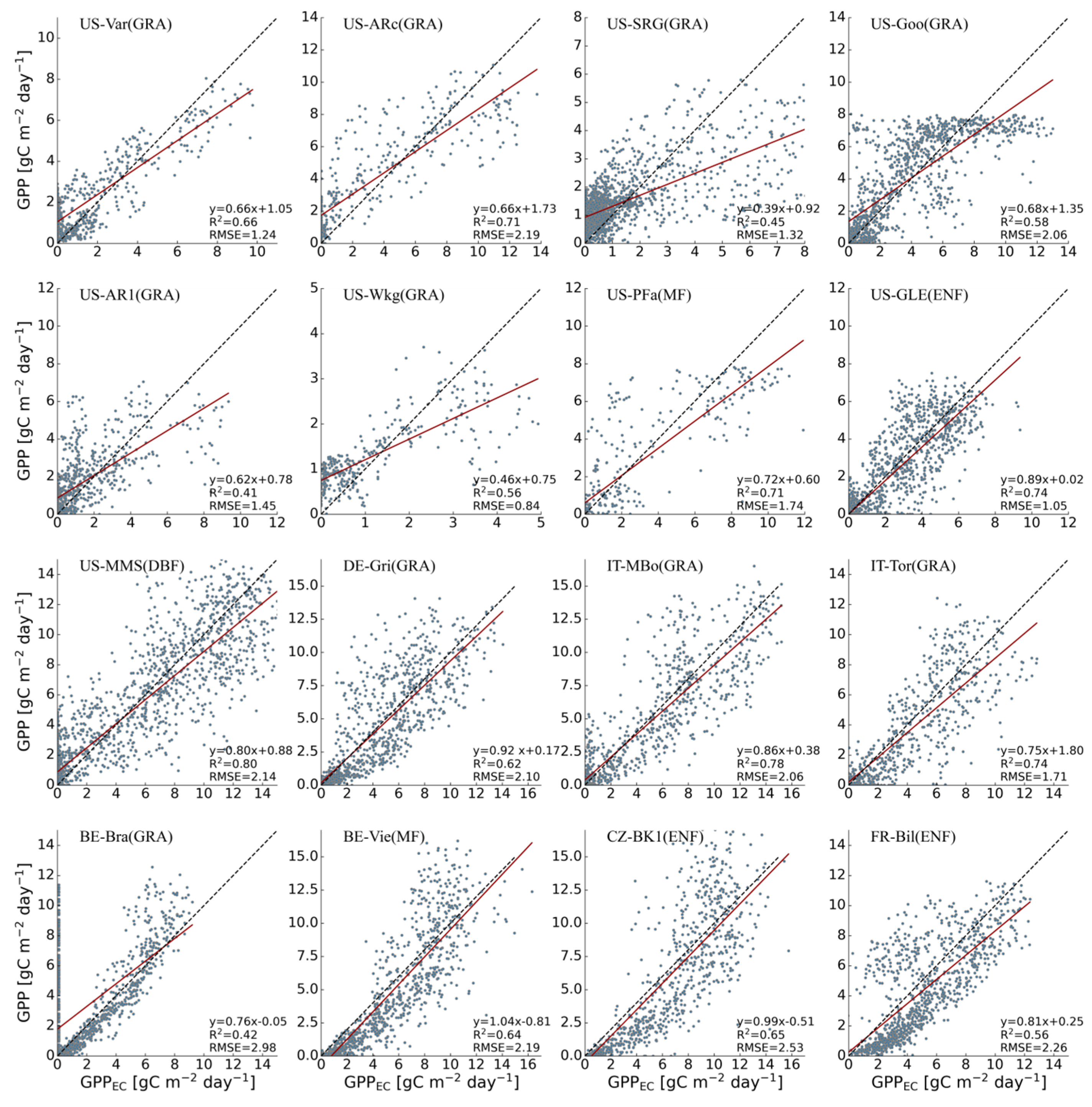
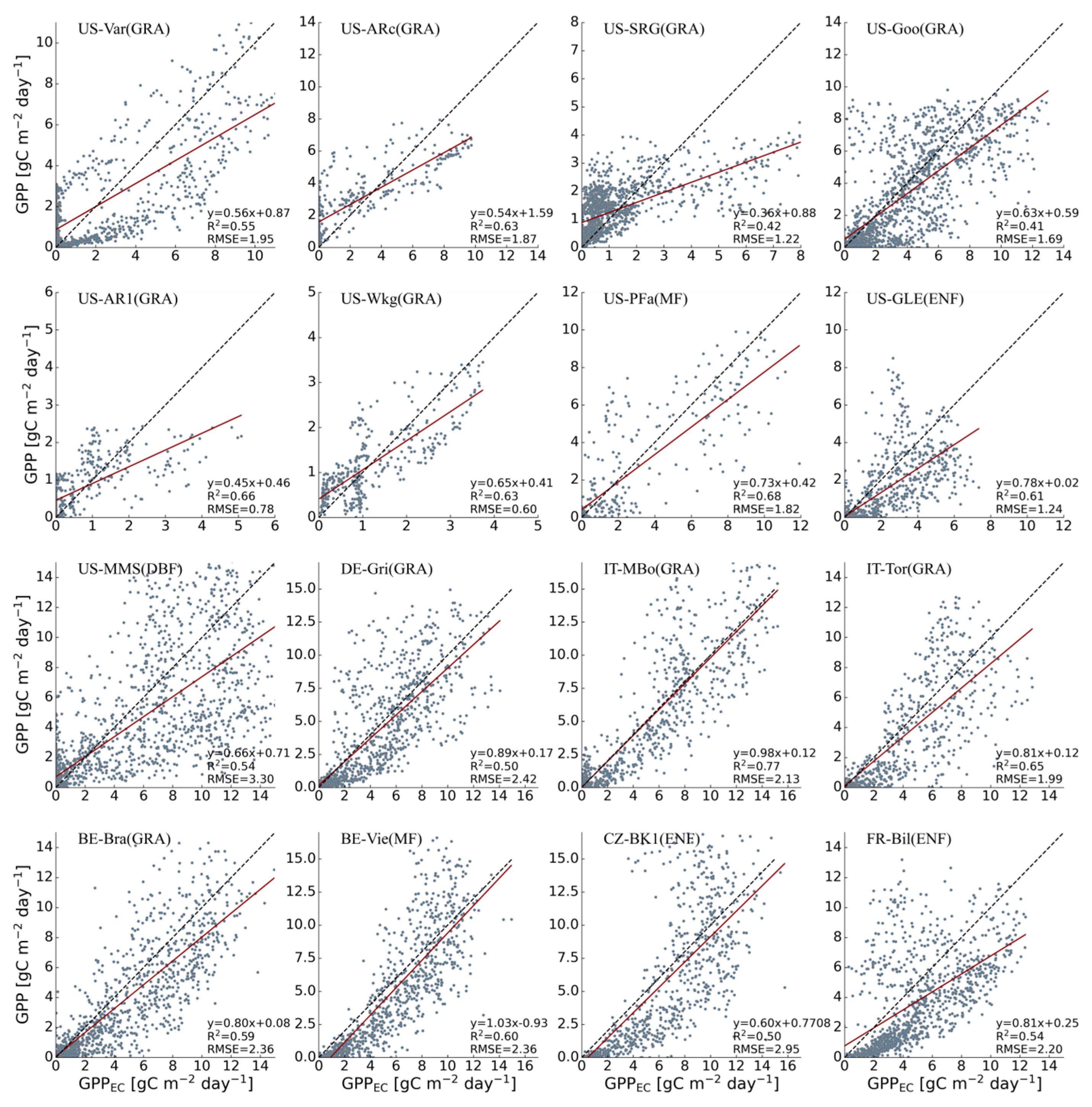
3.1. Performances of Original Models

After calibrating the TL-LUE model and VPM using the reference data, validation using the data for the remaining years was conducted (Figure 4 and Figure 5). The TL-LUE model performed the best at the US-MMS site (R² = 0.80, RMSE = 2.14 gCm⁻² day⁻¹) and performed the worst at US-AR1 (R² = 0.41, RMSE = 1.45 gCm⁻² day⁻¹). In general, the model showed significantly better performances at forest sites (R² ranged from 0.56 to 0.80, mean R² = 0.68) than at grass-type sites (R² ranged from 0.41 to 0.78, mean R² = 0.60). VPM performed the best at the forest site of IT-Mbo (R² = 0.77, RMSE = 2.13 gCm⁻² day⁻¹) while the worst at the grass-type site of US-Goo (R² = 0.41, RMSE = 1.69 gCm⁻² day⁻¹). Different from the TL-LUE model, for VPM, the overall performance for the forest sites (mean R² = 0.58) was similar to that of the grass-type sites (mean R² = 0.58).

From these results, it can be seen that the two models exhibited consistently good or poor performances at some sites due to the similarity in their model structures. For example, the two models performed less satisfactorily at the sites of US-SRG and US-Goo, with R² < 0.5; both show consistently good performances at the US-PFa and IT-Mbo sites (R² > 0.6). Meanwhile, due to the differences in input data, significant differences existed between the performances of the two models at the same site. VPM performed better (R² = 0.66, RMSE = 0.78 gCm⁻² day⁻¹) than the TL-LUE model (R² = 0.41, RMSE = 1.45 gCm⁻² day⁻¹) at the US-AR1 site.

3.2. Evaluation of Improved Models

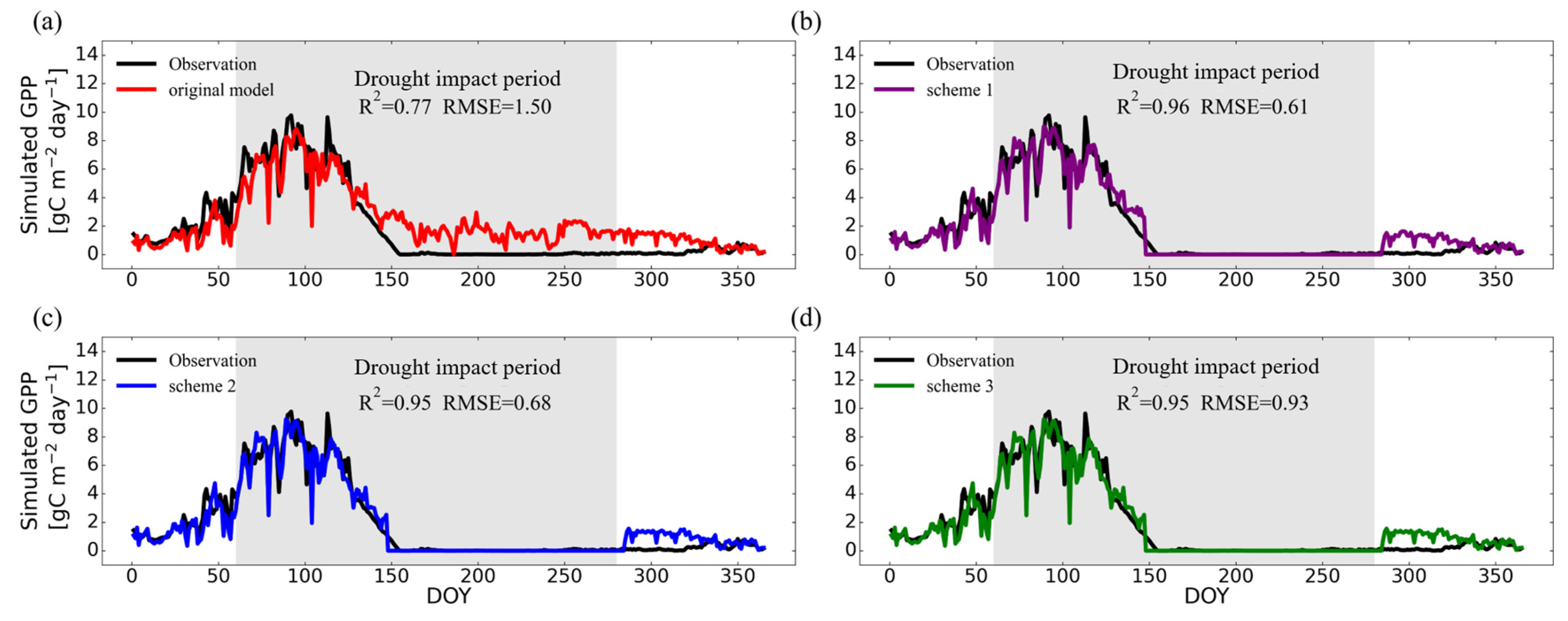
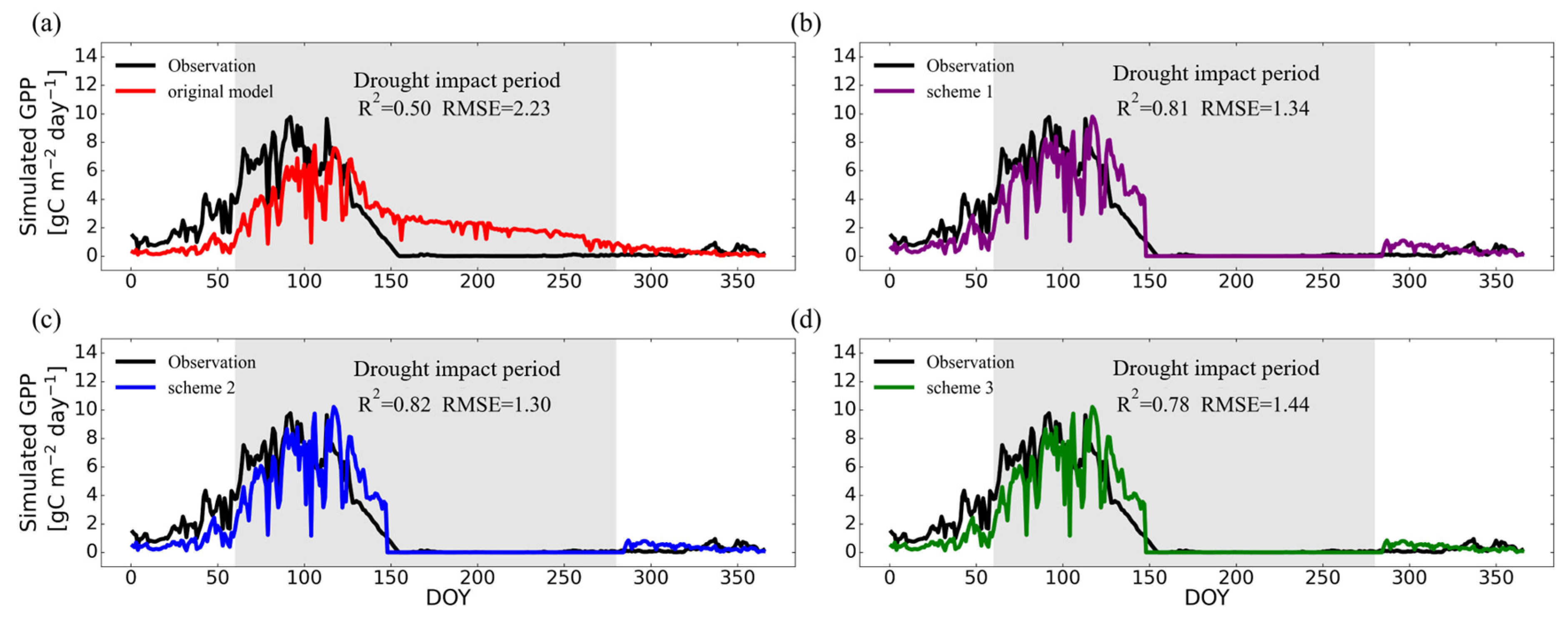
3.2.1. Temporal Variations on Typical Site

Figure 6 shows the simulated daily GPP over the year 2007 by the TL-LUE model with different modeling schemes for incorporating SM information at the grass-type site of US-Var. For the original TL-LUE model, although the simulations highly agreed with the observations during the initial drought period from the day of the year (DOY) 55 to 140, the simulations greatly overestimated from DOY 140 to 280 (Figure 6a). After incorporating SM information, all the simulations with different schemes showed clear improvements (Figure 6b–d). For these three schemes, a greatly improved performance was observed, especially during DOY 140 to 280. For Scheme 1, R² raised about 0.19, and RMSE dropped about 0.89 gCm⁻² day⁻¹. For Scheme 2, R² improved from 0.77 to 0.95, and RMSE decreased from 1.50 to 0.68 gCm⁻² day⁻¹. For Scheme 3, R² improved from 0.77 to 0.95, and RMSE decreased from 1.50 to 0.93 gCm⁻² day⁻¹. Overall, the simulations with Scheme 1 performed the best at the US-Var site.

Figure 7 shows the simulated daily GPP over the year 2007 by VPM at the US-Var site. The original VPM significantly underestimated GPP during the initial period, from DOY 55 to 140 (Figure 7a). However, it greatly overpredicted GPP during DOY 140 to 280, which is similar to the case of the TL-LUE model. Clear improvements were observed in the simulations incorporating SM information. For Scheme 1, R² raised from 0.50 to 0.81, and RMSE dropped from 2.23 gCm⁻² to 1.34 gCm⁻² day⁻¹ (Figure 7b). For Scheme 2, it was in high agreement with Scheme 1, but R² further raised to 0.82 and RMSE reduced to 1.30 gCm⁻² day⁻¹ (Figure 7c). The performance of Scheme 3 is slightly inferior to the first two schemes but also has a significant improvement over the original model, with an R² of 0.78 and RMSE of 1.44 gCm⁻² day⁻¹ (Figure 7d). Overall, the simulations with Scheme 2 had the best performance at the US-Var site.

We conducted similar analyses at other fifteen sites (Figure 8 and Figures S1–S15). We analyzed the improvements of R² and RMSE, i.e., the difference between the indexes of the best solution and the original model.

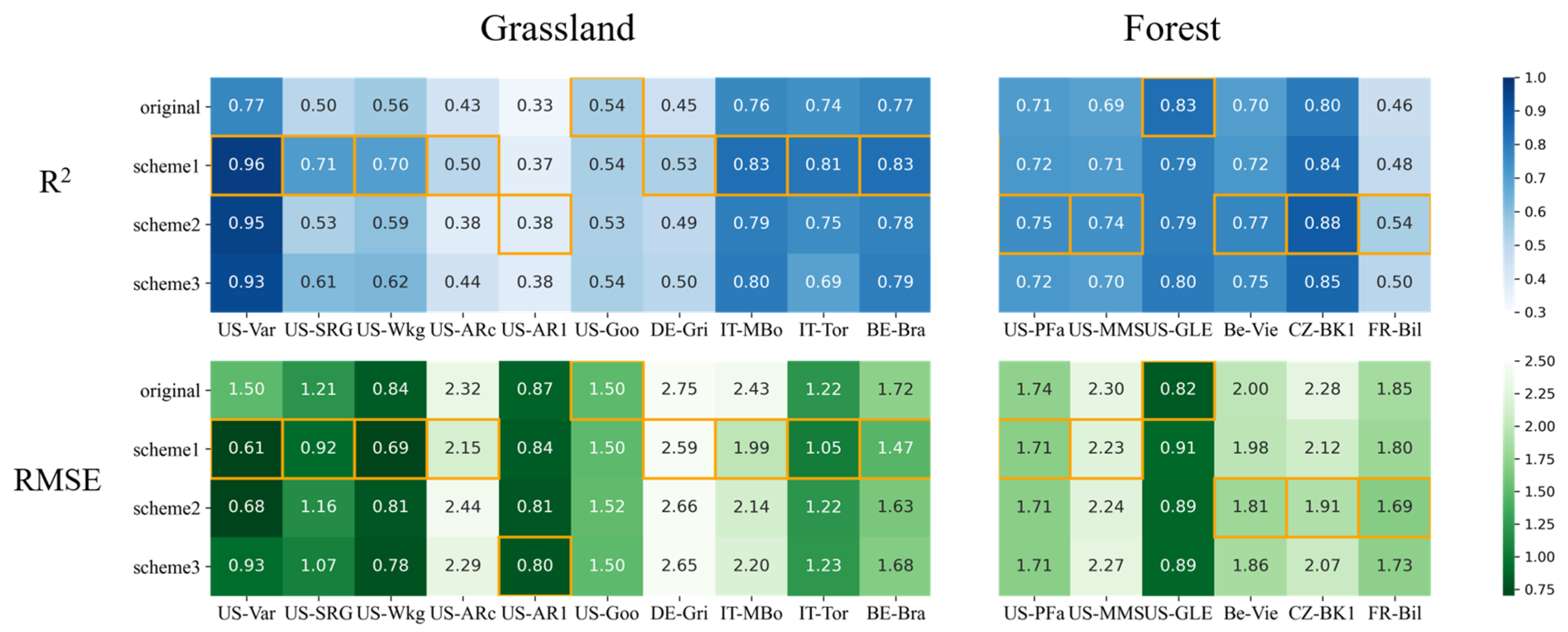
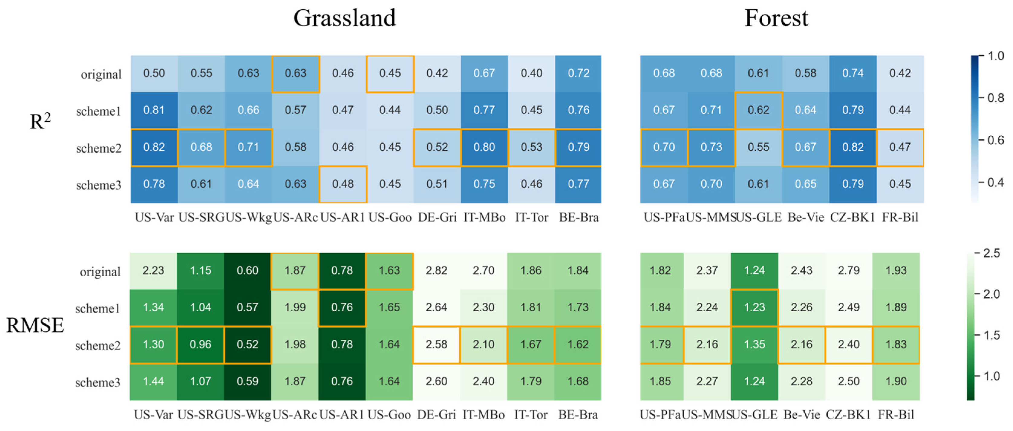
3.2.2. Improvements for Grass-Type Sites

For the TL-LUE model, the improvement solutions by incorporating SM showed different performances at various sites. For the grass-type, the simulations at most sites showed improvements compared to those by the original model, except for US-Goo (ΔR² = −0.01~0, ΔRMSE = 0~+0.02 gCm⁻² day⁻¹). The most significant improvement was observed at US-SRG (ΔR² = 0.21, ΔRMSE = −0.29 gCm⁻² day⁻¹), while at the other sites, the ΔR² of the improvement ranged from 0.05 to 0.2. A comparison of the different improvement schemes revealed that eight of the nine sites with significant improvements showed that Scheme 1 was the optimal scheme (except for US-AR1, where the optimal scheme was Scheme 2), i.e., it had the highest R² and the lowest RMSE.

For VPM, we conducted similar analysis at fifteen other sites (Figure 9 and Figures S1–S15). The simulations by incorporating SM performed differently at various sites. For the grass-type, 8 of the 10 sites showed an improvement over the original scheme (ΔR² = 0.02 to 0.32, ΔRMSE = −0.02 to −0.93 gCm⁻² day⁻¹), with the most pronounced improvement at the US-Var site (ΔR² = 0.32, ΔRMSE = 0.93 gCm⁻² day⁻¹). Among the eight sites with improvement, seven indicated that Scheme 2 was the best scheme, except for US-AR1 (the most significant improvement was in Scheme 3).

3.2.3. Improvements for Forest Sites

For the TL-LUE model, for the forest-type sites, the five sites, except for US-GLE, achieved the optimal simulation using Scheme 2. The improvements were generally less pronounced (ΔR² = 0.04–0.09) than the grass-type sites.

For VPM, in three forest sites, an improvement was observed at all 6 sites, with BE-Vie achieving the most significant improvement (ΔR² = 0.09, ΔRMSE = 0.27 gCm⁻² day⁻¹), whereas US-GLE showed very little improvement, and even Scheme 2 showed performance degradation. Moreover, all the other five sites except US-GLE showed Scheme 2 as the optimal improvement scheme.

3.2.4. Improvements for Non-Drought Periods

In addition, in order to verify the applicability of the scheme in non-drought periods, we analyzed the simulations for different improvement schemes by the two LUE models in different ecosystems during non-drought periods (Figure 10). It showed that among the 10 sites in the grassland, for the TL-LUE model, Scheme 1 had the highest R² and the lowest RMSE, while for VPM, Scheme 2 proved to be the best scheme. Among the six forest sites, for both TL-LUE and VPM, Scheme 2 showed the largest improvement in the simulations.

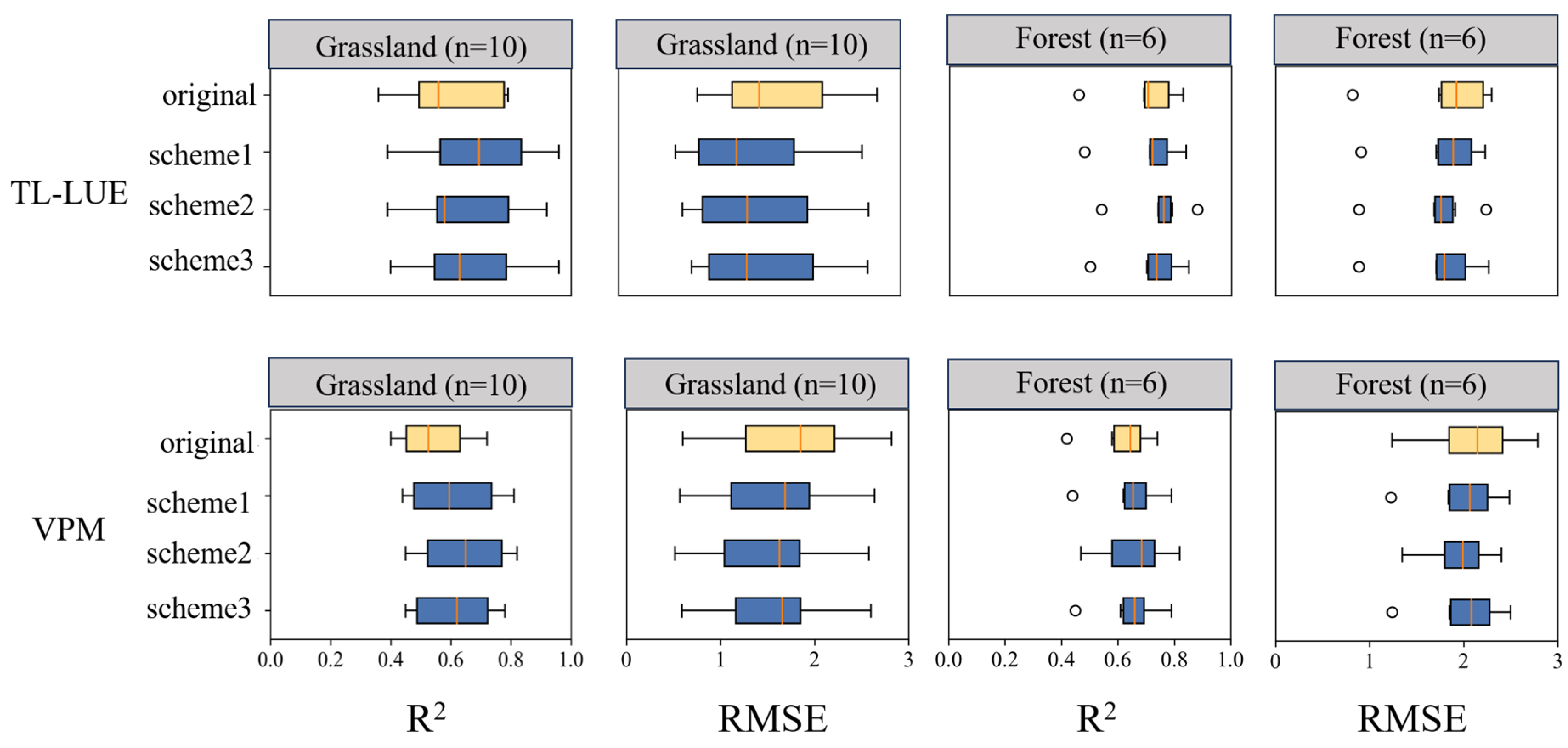
3.3. Improvement Comparison Between TL-LUE and VPM

Based on the results of Section 3.1 and Section 3.2, we found that TL-LUE and VPM have a general consistency, but there were some obvious differences. Thus, we further compared the performance between the two models by calculating the difference between the R² and RMSE values of the two models (ΔR², ΔRMSE) at each site (Figure 11). It showed that the superiority or inferiority of the TL-LUE model versus VPM on grass ecosystems varied across sites. Among the sixe sites in North America, the original TL-LUE model simulations were inferior to those of the original VPM at four sites (ΔR² = −0.05 to −0.20, ΔRMSE = 0.21 to 1.69 gCm⁻² day⁻¹). In contrast, the TL-LUE model outperformed VPM at grass-type sites in Europe. We also found that VPM generally outperformed the TL-LUE model with Scheme 2, both at the sites in North America and Europe. For the TL-LUE model, Scheme 2 accounted for both VPD and SM, whereas for VPM, it accounted for both LSWI and SM. For forest-type sites, both in North America and Europe, the original TL-LUE model performed significantly better than VPM (ΔR² = 0.01~−0.22, ΔRMSE = −0.08 to −0.51 gCm⁻² day⁻¹). Therefore, we conjecture whether the combination of LSWI and SM is superior to that of VPD and SM for grass-type sites and whether VPD better characterizes water stress for forest-type sites.

To test this hypothesis, we examined the correlation between in situ observations of GPP and various moisture indicators (e.g., LSWI, SM, VPD) during drought years (

Table 2. Correlation of various water stress indicators with GPP at flux sites.

Site	R(GPPobs-LSWI)	R(GPPobs-VPD)	R(GPPobs-SM)
US-Var	0.88	−0.39	0.40
US-SRG	0.61	−0.02	0.21
US-Wkg	0.63	0.11	0.29
US-ARc	0.84	0.17	0.28
US-AR1	0.39	0.19	0.29
US-Goo	0.75	0.26	0.05
FR-TOU	0.78	0.14	0.45
DE-Gri	0.69	0.18	0.39
IT-MBo	0.72	0.24	0.44
IT-Tor	0.79	0.26	0.51
BE-Bra	0.63	0.11	0.32
US-PFa	0.14	0.64	0.18
US-MMS	0.86	0.57	0.36
BE-Vie	0.36	0.67	0.23
US-GLE	0.23	0.77	0.08
CZ-BK1	0.14	0.82	0.28
FR-Bil	0.24	0.78	0.30

). The GPP at all ten grass-type sites exhibited the strongest correlation with LSWI. Differently, at forest sites, the GPP displayed the strongest correlation with VPD. Therefore, we speculate that for grass-type sites, VPD may be responsible for the worse performance of the scheme multiplying VPD and SM in the TL-LUE model. On the other hand, incorporating VPD into VPM might improve the GPP simulation for forests. To support this perspective, we analyzed the use of different moisture indicators in the TL-LUE model at the grass-type sites and in VPM at the forest sites (Figure 12, Figure 13 and Figures S16–S31). For the TL-LUE model, we conducted the simulations at the grass-type sites using four different moisture indicators: VPD, LSWI, SM, and LSWI*SM (Figure 12). The results indicate that replacing VPD with LSWI in the TL-LUE model led to substantial improvements. For instance, at the US-Var site, replacing VPD with LSWI resulted in an increase of R² by about 0.2 with a decrease in RMSE by 0.90 gCm⁻² day⁻¹. Combining the results of the improvements at the 10 grass-type sites, 3 had an increase in R² of 0.1 to 0.2 (US-Var, US-SRG, and US-Wkg), and the remaining 7 sites had changes in R² of 0.02 to 0.07. For the grassland sites, the maximum R², the minimum R², and the average value of R², as well as the RMSE simulated by the SM*LSWI scheme at all the sites, performed best among all the schemes. Therefore, the SM*LSWI scheme was the optimal scheme for the grassland sites, followed by the schemes LSWI and SM, and the scheme considering only VPD showed the poorest performance. At the US-SRG site, the scheme multiplying LSWI with SM was higher in R² by 0.06 with lower RMSE by 0.11 gCm⁻² day⁻¹ than the scheme using only SM. This was also verified by the results at all 10 grass-type sites, which showed an increase of R² by 0.0 to 0.09 and a decrease in RMSE by 0.01 to 0.2 gCm⁻² day⁻¹. For all six forest sites, replacing LSWI with VPD in VPM also showed an improvement over the original model (Figure 13). For example, at the US-GLE site, R² increased by 0.07 while RMSE decreased by 0.12 gCm⁻² day⁻¹. At all six sites, R² improved by 0.02 to 0.09 and RMSE decreased by 0.03 to 0.36 gCm⁻² day⁻¹. For the forest sites, the results by the schemes SM*VPD and VPD coincided very well, but the SM*VPD scheme still performed slightly better than the VPD scheme, and they both clearly outperformed the schemes LSWI and SM*LSWI.

4. Discussion

4.1. The Added Value of Incorporating Soil Moisture Information

Under drought conditions, LUE models generally appear to overestimate GPP, with obvious inter-model differences at the same sites. This is mainly associated with the diverse ways among different LUE models in characterizing the response to moisture stresses, which is a main factor affecting GPP during drought periods [4]. For example, the TL-LUE model uses VPD while VPM utilizes LSWI. According to our study, the simulation results improved after incorporating LSWI into the TL-LUE model, which can be explained by a better capacity of LSWI to decipher drought impacts than that of VPD for grass-type ecosystems [44]. However, for forest ecosystems, the TL-LUE model has overall superior performance than VPM, for both including and not including SM, which may associate with the better capacities of either VPD in characterizing drought impact or the two-leaf schemes in characterizing complex radiation regimes among vegetation canopies.

For the TL-LUE model, there was a substantial improvement at most grass-type sites after replacing VPD with SM. VPD is sensitive to air temperature and it is challenging to characterize the effect of soil water deficit on vegetation growth during extreme drought. In addition, grass-type ecosystems have relatively short root lengths and face more difficulties in drawing water from deeper soil layers [45], thus, they are largely dependent on surface SM. Bayat B improved the SCOPE model by integrating soil moisture data, creating SCOPE-SM to better capture water stress effects on photosynthesis and evapotranspiration under drought. Validation at the US-Var Fluxnet site shows significant accuracy improvements, emphasizing the value of soil moisture observations, which aligns with this study’s findings on the critical role of soil moisture in enhancing GPP simulations for grass-type ecosystems [46]. Thus, the response of the LUE model to drought can be better improved by using the surface SM measurements at the site scale. At all forest sites, the results of the various improvement schemes were very similar to the original model. It should be noted that even at the US-GLE site, the simulations with the original model were better than those with improvement schemes. In forest ecosystems, the vegetation is taller and has a greater number of biomes, where various types of water exist, including a greater proportion of atmospheric water, and the vegetation roots are longer and can draw water from deeper soils. Therefore, the incorporation of surface SM might have only a minimal effect on the improvement of GPP simulations.

For VPM, the GPP simulations were improved at most grass-type sites. The results also provide further evidence that SM has a critical influence on the vegetation growth of grass-type ecosystems during dry periods. The results for the US-Var site and the US-SRG site indicate that considering the effects of both SM and LSWI in VPM can substantially improve GPP simulations. Moreover, the scheme multiplying LSWI and SM produced the best performance. This may be because LSWI is only able to represent the water content status in leaves, whereas during extreme droughts, vegetation growth is controlled by both leaf water and SM availabilities [47]. Pei’s study also highlights that plant water stress (measured by LSWI, EF, PM, etc.) influences stomatal conductance and regulates evapotranspiration and photosynthesis, which are crucial for accurately modeling GPP. Atmospheric water stress is often included in models like MOD17 and EC-LUE, while soil moisture and plant water stress are key in models such as GLO-PEM and VPM, reinforcing the importance of integrating these proxies, especially soil moisture, into ecosystem flux models [48]. The use of the LSWI*SM scheme in the TL-LUE model led to the best simulations at all four grass-type sites (Figure 10), which confirmed this viewpoint. At the US-GLE site, all three schemes were inferior to the original model, which is similar to the case for the TL-LUE model, suggesting that surface SM may not be the dominant factor for vegetation growth in less drought-vulnerable ecosystems like forests.

4.2. Implications for Future LUE Model Development

During dry periods, vegetation growth is mainly limited by moisture factors, and appropriate moisture factors must be applied towards an accurate simulation of GPP [47]. The experimental results showed that after incorporating SM, both LUE models achieved improved GPP simulations at most sites.

For grass-type ecosystems, LSWI should be preferred to characterize water stress, but in drought periods, better simulations can be obtained using the scheme multiplying LSWI with SM. For forest ecosystems, there is typically a strong correlation between GPP and VPD. The simulation results using VPD in both models also demonstrate better performance at most sites. Additionally, the impact of drought on grass-type ecosystems can be effectively characterized by surface SM, while it is less effective for forest ecosystems. Hence, distinct water indicators should be applied to different ecosystem types.

When both models considered LSWI and SM as water stress indicators for grass-type, we found that the TL-LUE model outperformed VPM at many sites (e.g., US-Wkg and US-SRG). In addition, at the forest sites, the simulations by VPM after replacing LSWI with VPD showed some improvement but were still slightly worse than the TL-LUE model. Given the same input meteorological data (e.g., air temperature) and remote sensing data (e.g., LAI and reflectance), much of the difference in results may stem from the fact that the TL-LUE results considering sunlit and shaded leaves may be superior to the large leaf model [49]. Vegetation canopy consists of shade and sunlit leaves, and they receive different amounts of direct and diffuse incident solar radiation [50,51], so they have different structures as well as light saturation points. Thus, considering the distinction between shade and sun leaves in the LUE model may also improve the simulation accuracy.

4.3. Biodiversity Recovery, Ecosystem Functioning, and Sustainability

In the context of improving GPP (gross primary productivity) simulations under drought conditions, the incorporation of soil moisture (SM) and vegetation indices such as LSWI significantly enhances the accuracy of carbon flux predictions. Furthermore, these improvements have profound implications for understanding biodiversity recovery, ecosystem functioning, and long-term sustainability, offering critical scientific insights and decision-making support.

Drought poses significant challenges to ecosystem resilience and biodiversity conservation, and accurate GPP modeling provides a quantitative framework for assessing ecosystem recovery processes under drought stress [52,53]. Grass-type ecosystems, due to their shallow root systems, are more reliant on surface SM and are particularly vulnerable to water deficits [54,55]. By integrating SM and LSWI into light-use efficiency (LUE) models, this study achieves a more precise simulation of productivity changes in these ecosystems during recovery periods. Such an approach enables more effective identification of critical periods and regions affected by drought stress, thereby informing restoration strategies, including optimized irrigation practices, vegetation coverage adjustments, or the introduction of drought-tolerant species. Moreover, accurately identifying water stress conditions across ecosystems facilitates the prioritization of restoration efforts in biodiversity hotspots, providing a scientific basis for protecting and rehabilitating critical habitats.

The varying responses of different ecosystems to drought stress indicators reflect the complex interactions among vegetation structure, root system distribution, photosynthetic physiology, and water-use strategies. By integrating SM and LSWI, this study elucidates the response mechanisms of ecosystem functioning to water stress. For instance, the carbon sequestration capacity of grass-type ecosystems is particularly sensitive to surface water availability during drought periods, as evidenced by improved GPP simulations. This highlights the dependency of grass-type ecosystems’ primary productivity and carbon cycling on short-term hydrological conditions, especially dynamic changes in surface soil moisture [56].

In contrast, forest ecosystems exhibit a stronger correlation between GPP and vapor pressure deficit (VPD), which underscores the importance of atmospheric moisture dynamics in influencing their photosynthetic efficiency and water-use strategies. Additionally, the complex light environment within forest canopies (e.g., the distribution and varying light saturation points of sunlit and shaded leaves) plays a significant role in carbon flux processes. The ability of LUE models to differentiate these complex mechanisms not only deepens our understanding of ecosystem processes but also offers new pathways for further model optimization.

In the face of intensifying global climate change and increasing drought frequency, achieving sustainable ecosystem management is a critical challenge. The incorporation of SM and LSWI into LUE models not only improves simulation accuracy but also provides quantitative insights for evaluating and managing ecosystem services. For grass-type ecosystems, where GPP is highly sensitive to surface SM, sustainable practices such as soil conservation, water resource management, and irrigation optimization become essential for enhancing drought resilience. Specific measures, including soil mulching, increasing water storage capacity, and regulating irrigation schedules, can strengthen the adaptive capacity of grass-type ecosystems.

For forest ecosystems, the study suggests that adaptive strategies focusing on atmospheric water dynamics (e.g., VPD) and canopy microenvironments may be more effective in mitigating drought stress. Particularly in forest ecosystems with relatively low drought vulnerability, the study shows limited improvement from model enhancements, highlighting the need for future management practices to consider the structural complexity and hydrological dynamics of forest systems.

In summary, the model improvements proposed in this study represent significant advancements not only in carbon cycling simulations but also in supporting biodiversity conservation, enhancing ecosystem resilience, and achieving sustainable ecosystem management. By tailoring water stress indicators to the unique characteristics of different ecosystems, this approach provides both a scientific foundation for addressing global environmental challenges and a practical paradigm for optimizing regional ecosystem services.

4.4. Uncertainties

Some uncertainties exist in this study. First, the SM measurements provided by the flux network are a single point of data and may not represent the soil water status of the flux footprint of the flux tower well. Second, the values obtained using the physicochemical properties of the site soil when calculating the field water holding capacity and permanent wilting point of the site are obtained directly from off-the-shelf products because not all sites provide soil data, which may lead to some uncertainties. These uncertainties could be alleviated when more in situ observations are available in the future.

5. Conclusions

In this study, in order to improve the GPP simulation under water stresses by LUE models, we constructed three different water stress improvement schemes with a fused SM function f(SM) as the core. An attempt was made to explore which scheme best optimizes the simulation of GPP by the two LUE models during drought periods on different ecosystem types. The SWOT analysis provides a clearer understanding of the strengths and weaknesses of each scheme, highlighting their suitability for different ecosystems (Table 3). The main findings are as follows:

(1)

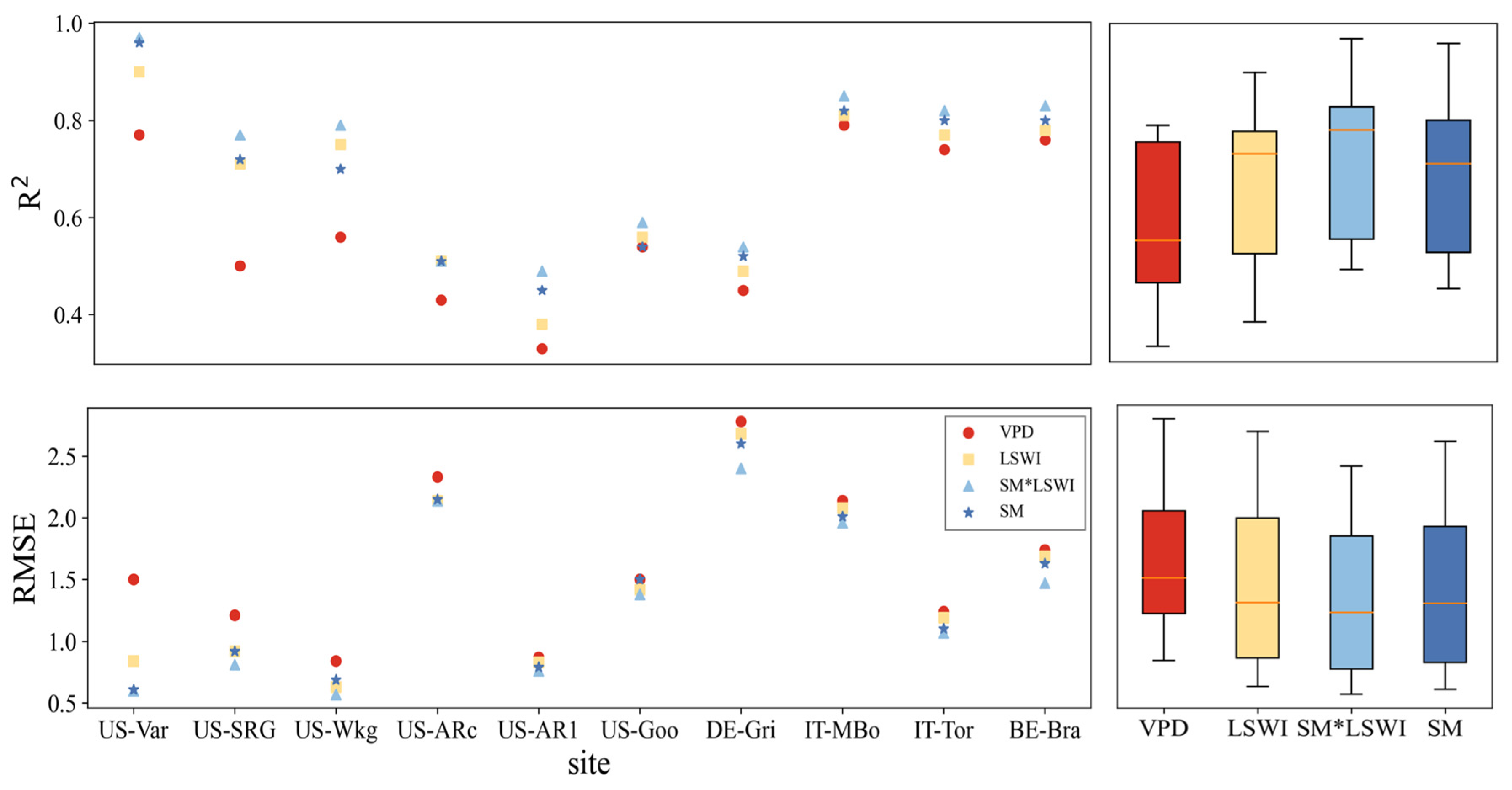
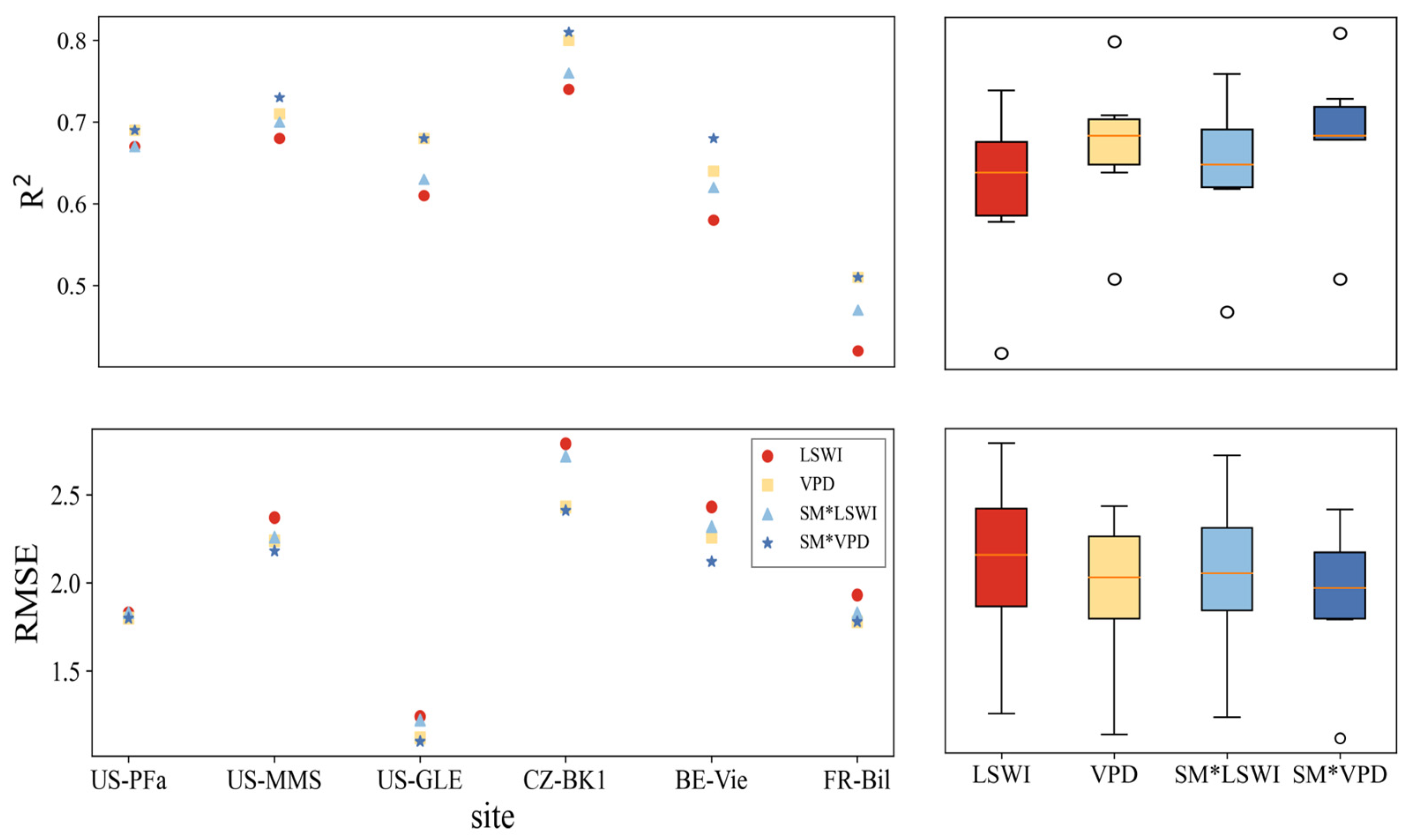
At most grass-type sites, VPM outperformed the TL-LUE model during drought periods, which is associated with the fact that LSWI responded better to drought than VPD at grass-type ecosystems. In contrast, at forest ecosystem sites, the TL-LUE model performed better, with VPD being more representative of water stress in forest ecosystems during drought periods.

(2)

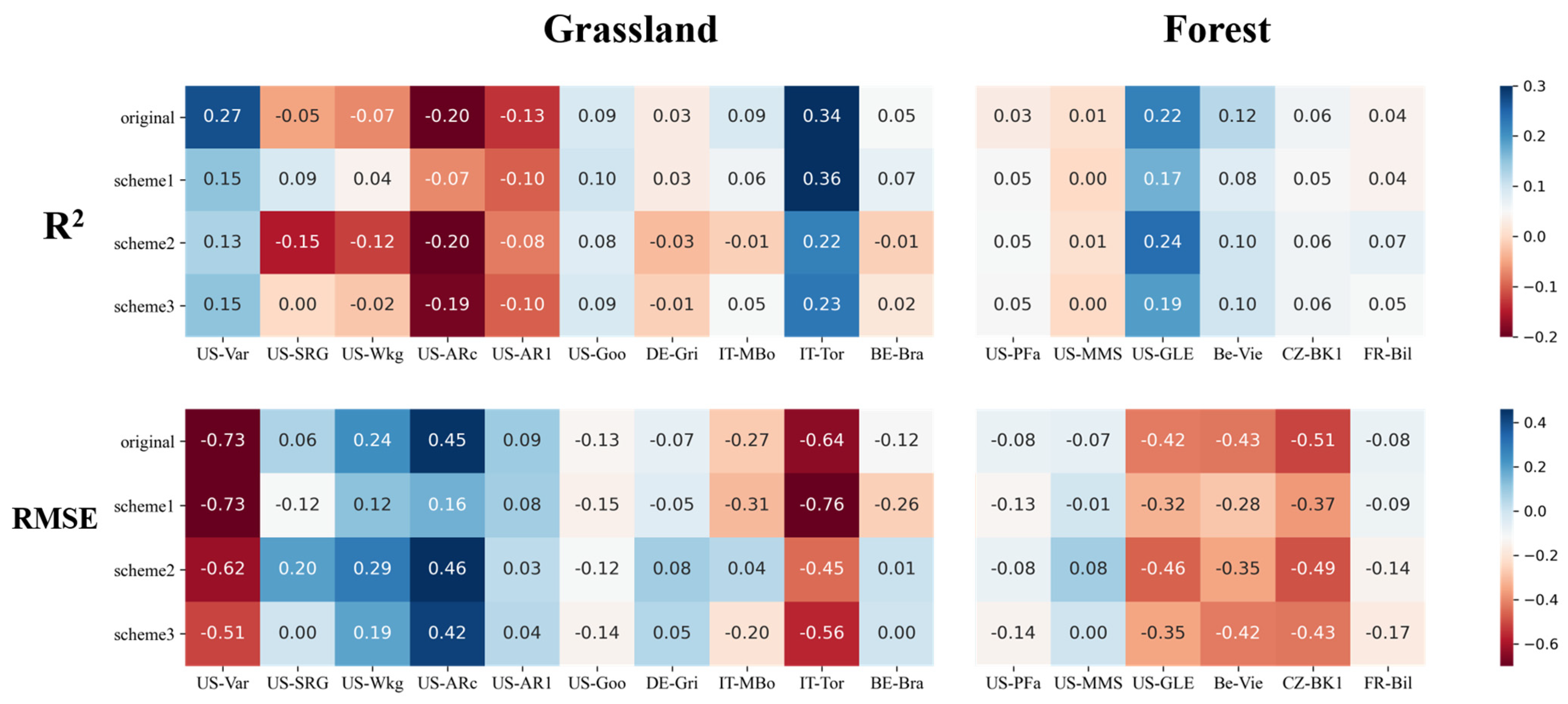
At grass-type sites, incorporating SM information by using a sigmoid-type SM correction function f(SM) led to clear improvements for both LUE models, in particular with the scheme multiplying f(SM) with LSWI. The TL-LUE model exhibited a maximum increase in R² of 0.27 (+54%) and a maximum decrease in RMSE of 0.40 gCm⁻² day⁻¹ (−33%). VPM showed improvements in R² as large as 0.32 (+64%) with a decrease in RMSE at a maximum of 0.93 gCm⁻² day⁻¹ (−41%).

(3)

In comparison, for forest ecosystems, it was more challenging to improve LUE models with SM under water stresses (for TL-LUE: ΔR² = −0.04~0.08, ΔRMSE = +0.07~−0.37 gCm⁻² day⁻¹; and for VPM, ΔR² = 0.01~0.08, ΔRMSE = −0.01~−0.39 gCm⁻² day⁻¹), since forests are less sensitive to surface SM variation. In addition, in contrast to grass-type ecosystems, using VPD as a moisture indicator in VPM can better improve forest GPP simulations under water stresses than using LSWI.

Table 3. SWOT analysis of different improvement schemes for LUE models.

	Scheme 1	Scheme 2	Scheme 3
Strengths	Best performance for grass-type ecosystems. Simple and effective for capturing surface soil moisture.	Best overall performance for both grasslands and forests. Performs well during non-drought and drought periods.	Balanced improvement across ecosystems. Effective in grasslands under certain conditions.
Weakness	Less effective for forests (minimal improvement at forest sites). Limited in representing leaf moisture.	High data requirements (e.g., soil moisture and LSWI data). Slightly lower performance for grasslands at some sites.	Inferior to Scheme 1 and Scheme 2 at most sites. Less significant improvements during drought periods.
Opportunities	Can be widely applied in drought-prone grasslands. Easily extendable with more surface soil moisture data.	Promising for ecosystem-level GPP modeling in diverse regions. Can be further improved with advanced data fusion.	Useful for regions with mixed water stress impacts. Potential to refine for grassland ecosystems.
Threats	Performance highly dependent on surface soil moisture data quality. May not generalize to forest ecosystems.	Requires advanced remote sensing for LSWI and soil moisture integration. High computational cost for broader applications.	May fail to outperform simpler models. Less adaptable to varying climatic conditions.

Table 3. SWOT analysis of different improvement schemes for LUE models.

	Scheme 1	Scheme 2	Scheme 3
Strengths	Best performance for grass-type ecosystems. Simple and effective for capturing surface soil moisture.	Best overall performance for both grasslands and forests. Performs well during non-drought and drought periods.	Balanced improvement across ecosystems. Effective in grasslands under certain conditions.
Weakness	Less effective for forests (minimal improvement at forest sites). Limited in representing leaf moisture.	High data requirements (e.g., soil moisture and LSWI data). Slightly lower performance for grasslands at some sites.	Inferior to Scheme 1 and Scheme 2 at most sites. Less significant improvements during drought periods.
Opportunities	Can be widely applied in drought-prone grasslands. Easily extendable with more surface soil moisture data.	Promising for ecosystem-level GPP modeling in diverse regions. Can be further improved with advanced data fusion.	Useful for regions with mixed water stress impacts. Potential to refine for grassland ecosystems.
Threats	Performance highly dependent on surface soil moisture data quality. May not generalize to forest ecosystems.	Requires advanced remote sensing for LSWI and soil moisture integration. High computational cost for broader applications.	May fail to outperform simpler models. Less adaptable to varying climatic conditions.

The significance of this study lies in the construction and comparison of three different water stress improvement schemes, demonstrating how incorporating SM information can improve GPP simulation under water stress across different ecosystem types. This provides valuable insights for future research, showing that different water stress schemes should be applied to different ecosystem types, particularly grasslands and forests, to improve GPP simulation accuracy and adaptability. Specifically, the improvement schemes incorporating SM information showed significant results for grassland ecosystems, offering a reference for future ecological modeling and climate change studies.

While this study has achieved promising results, there is still room for improvement. Future research could explore how these improvement schemes can be extended to other ecosystem types, especially considering regional and climatic variations in model performance. Additionally, as more soil and meteorological data become available, the methods used in this study can be further refined. Given the impact of climate change on water availability in ecosystems, future work should focus on incorporating climate change factors into models to further improve GPP simulation accuracy and predictive capabilities.

In conclusion, this study significantly improves GPP simulation during drought periods by incorporating SM information into LUE models. The findings indicate that SM plays a particularly critical role in grassland ecosystems, whereas forest ecosystems require more adaptable moisture indicators and methods. These results provide an important theoretical foundation and practical significance for future ecological modeling, climate change research, and related policy development.

References

1. Li, X.; Xiao, J. A Global, 0.05-Degree Product of Solar-Induced Chlorophyll Fluorescence Derived from OCO-2, MODIS, and Reanalysis Data. Remote Sens. 2019, 11, 517. [Google Scholar] [CrossRef]
2. He, B.; Liu, J.; Guo, L.; Wu, X.; Xie, X.; Zhang, Y.; Chen, C.; Zhong, Z.; Chen, Z. Recovery of Ecosystem Carbon and Energy Fluxes From the 2003 Drought in Europe and the 2012 Drought in the United States. Geophys. Res. Lett. 2018, 45, 4879–4888. [Google Scholar] [CrossRef]
3. Lv, Y.; Liu, J.; He, W.; Zhou, Y.; Tu Nguyen, N.; Bi, W.; Wei, X.; Chen, H. How Well Do Light-Use Efficiency Models Capture Large-Scale Drought Impacts on Vegetation Productivity Compared with Data-Driven Estimates? Ecol. Indic. 2023, 146, 109739. [Google Scholar] [CrossRef]
4. Stocker, B.D.; Zscheischler, J.; Keenan, T.F.; Prentice, I.C.; Seneviratne, S.I.; Peñuelas, J. Drought Impacts on Terrestrial Primary Production Underestimated by Satellite Monitoring. Nat. Geosci. 2019, 12, 264–270. [Google Scholar] [CrossRef]
5. Zheng, Y.; Zhang, L.; Xiao, J.; Yuan, W.; Yan, M.; Li, T.; Zhang, Z. Sources of Uncertainty in Gross Primary Productivity Simulated by Light Use Efficiency Models: Model Structure, Parameters, Input Data, and Spatial Resolution. Agric. For. Meteorol. 2018, 263, 242–257. [Google Scholar] [CrossRef]
6. Ciais, P.; Reichstein, M.; Viovy, N.; Granier, A.; Ogée, J.; Allard, V.; Aubinet, M.; Buchmann, N.; Bernhofer, C.; Carrara, A.; et al. Europe-Wide Reduction in Primary Productivity Caused by the Heat and Drought in 2003. Nature 2005, 437, 529–533. [Google Scholar] [CrossRef]
7. Ghil, M.; Yiou, P.; Hallegatte, S.; Malamud, B.D.; Naveau, P.; Soloviev, A.A.; Friederichs, P.; Keilis-Borok, V.I.; Kondrashov, D.; Kossobokov, V.; et al. Extreme Events: Dynamics, Statistics and Prediction. Nonlinear Process. Geophys. 2011, 18, 295–350. [Google Scholar] [CrossRef]
8. Yuan, M.; Zhu, Q.; Zhang, J.; Liu, J.; Chen, H.; Peng, C.; Li, P.; Li, M.; Wang, M.; Zhao, P. Global response of terrestrial gross primary productivity to climate extremes. Sci. Total Environ. 2021, 750, 142337. [Google Scholar] [CrossRef]
9. Liu, S.; Chadwick, O.A.; Roberts, D.A.; Still, C.J. Relationships between GPP, satellite measures of greenness and canopy water content with soil moisture in Mediterranean-Climate Grassland and Oak Savanna. Appl. Environ. Soil Sci. 2011, 2011, 839028. [Google Scholar] [CrossRef]
10. Valjarević, A. GIS-Based Methods for Identifying River Networks Types and Changing River Basins. Water Resour. Manag. 2024, 38, 5323–5341. [Google Scholar] [CrossRef]
11. Zhang, Y.; Xiao, X.; Zhou, S.; Ciais, P.; McCarthy, H.; Luo, Y. Canopy and physiological controls of GPP during drought and heat wave. Geophys. Res. Lett. 2016, 43, 3325–3333. [Google Scholar] [CrossRef]
12. Breshears, D.D.; Cobb, N.S.; Rich, P.M.; Price, K.P.; Allen, C.D.; Balice, R.G.; Romme, W.H.; Kastens, J.H.; Floyd, M.L.; Belnap, J.; et al. Regional vegetation die-off in response to global-change-type drought. Proc. Natl. Acad. Sci. USA 2005, 102, 15144–15148. [Google Scholar] [CrossRef]
13. Ji, L.; Peters, A.J. Assessing vegetation response to drought in the northern Great Plains using vegetation and drought indices. Remote Sens. Environ. 2003, 87, 85–98. [Google Scholar] [CrossRef]
14. Monteith, J.L. Solar Radiation and Productivity in Tropical Ecosystems. J. Appl. Ecol. 1972, 9, 747. [Google Scholar] [CrossRef]
15. Dong, J.; Xiao, X.; Wagle, P.; Zhang, G.; Zhou, Y.; Jin, C.; Torn, M.S.; Meyers, T.P.; Suyker, A.E.; Wang, J.; et al. Comparison of Four EVI-Based Models for Estimating Gross Primary Production of Maize and Soybean Croplands and Tallgrass Prairie under Severe Drought. Remote Sens. Environ. 2015, 162, 154–168. [Google Scholar] [CrossRef]
16. Wu, C.; Chen, J.M.; Desai, A.R.; Hollinger, D.Y.; Arain, M.A.; Margolis, H.A.; Gough, C.M.; Staebler, R.M. Remote Sensing of Canopy Light Use Efficiency in Temperate and Boreal Forests of North America Using MODIS Imagery. Remote Sens. Environ. 2012, 118, 60–72. [Google Scholar] [CrossRef]
17. Zhao, M.; Heinsch, F.A.; Nemani, R.R.; Running, S.W. Improvements of the MODIS Terrestrial Gross and Net Primary Production Global Data Set. Remote Sens. Environ. 2005, 95, 164–176. [Google Scholar] [CrossRef]
18. He, W.; Ju, W.; Jiang, F.; Parazoo, N.; Gentine, P.; Wu, X.; Zhang, C.; Zhu, J.; Viovy, N.; Jain, A.K.; et al. Peak Growing Season Patterns and Climate Extremes-Driven Responses of Gross Primary Production Estimated by Satellite and Process Based Models over North America. Agric. For. Meteorol. 2021, 298–299, 108292. [Google Scholar] [CrossRef]
19. Wei, X.; He, W.; Zhou, Y.; Cheng, N.; Xiao, J.; Bi, W.; Liu, Y.; Sun, S.; Ju, W. Increased Sensitivity of Global Vegetation Productivity to Drought Over the Recent Three Decades. J. Geophys. Res. Atmos. 2023, 128, e2022JD037504. [Google Scholar] [CrossRef]
20. Stocker, B.D.; Zscheischler, J.; Keenan, T.F.; Prentice, I.C.; Peñuelas, J.; Seneviratne, S.I. Quantifying Soil Moisture Impacts on Light Use Efficiency across Biomes. New Phytol. 2018, 218, 1430–1449. [Google Scholar] [CrossRef]
21. Green, J.K.; Seneviratne, S.I.; Berg, A.M.; Findell, K.L.; Hagemann, S.; Lawrence, D.M.; Gentine, P. Large Influence of Soil Moisture on Long-Term Terrestrial Carbon Uptake. Nature 2019, 565, 476–479. [Google Scholar] [CrossRef] [PubMed]
22. Liu, X.; Feng, X.; Fu, B. Changes in Global Terrestrial Ecosystem Water Use Efficiency Are Closely Related to Soil Moisture. Sci. Total Environ. 2020, 698, 134165. [Google Scholar] [CrossRef] [PubMed]
23. Verhoef, A.; Egea, G. Modeling Plant Transpiration under Limited Soil Water: Comparison of Different Plant and Soil Hydraulic Parameterizations and Preliminary Implications for Their Use in Land Surface Models. Agric. For. Meteorol. 2014, 191, 22–32. [Google Scholar] [CrossRef]
24. Ju, W.; Chen, J.M.; Black, T.A.; Barr, A.G.; Liu, J.; Chen, B. Modelling Multi-Year Coupled Carbon and Water Fluxes in a Boreal Aspen Forest. Agric. For. Meteorol. 2006, 140, 136–151. [Google Scholar] [CrossRef]
25. Yan, H.; Wang, S.; Huete, A.; Shugart, H.H. Effects of Light Component and Water Stress on Photosynthesis of Amazon Rainforests During the 2015/2016 El Niño Drought. J. Geophys. Res. Biogeosci. 2019, 124, 1574–1590. [Google Scholar] [CrossRef]
26. Yuan, W.; Liu, S.; Zhou, G.; Zhou, G.; Tieszen, L.L.; Baldocchi, D.; Bernhofer, C.; Gholz, H.; Goldstein, A.H.; Goulden, M.L.; et al. Deriving a Light Use Efficiency Model from Eddy Covariance Flux Data for Predicting Daily Gross Primary Production across Biomes. Agric. For. Meteorol. 2007, 143, 189–207. [Google Scholar] [CrossRef]
27. Jones, L.A.; Kimball, J.S.; Reichle, R.H.; Madani, N.; Glassy, J.; Ardizzone, J.V.; Colliander, A.; Cleverly, J.; Desai, A.R.; Eamus, D.; et al. The SMAP Level 4 Carbon Product for Monitoring Ecosystem Land–Atmosphere CO2Exchange. IEEE Trans. Geosci. Remote Sens. 2017, 55, 6517–6532. [Google Scholar] [CrossRef]
28. Madani, N.; Parazoo, N.C.; Kimball, J.S.; Ballantyne, A.P.; Reichle, R.H.; Maneta, M.; Saatchi, S.; Palmer, P.I.; Liu, Z.; Tagesson, T. Recent Amplified Global Gross Primary Productivity Due to Temperature Increase Is Offset by Reduced Productivity Due to Water Constraints. AGU Adv. 2020, 1, e2020AV000180. [Google Scholar] [CrossRef]
29. He, M.; Kimball, J.S.; Running, S.; Ballantyne, A.; Guan, K.; Huemmrich, F. Satellite Detection of Soil Moisture Related Water Stress Impacts on Ecosystem Productivity Using the MODIS-Based Photochemical Reflectance Index. Remote Sens. Environ. 2016, 186, 173–183. [Google Scholar] [CrossRef]
30. Wang, S.; Ibrom, A.; Bauer-Gottwein, P.; Garcia, M. Incorporating Diffuse Radiation into a Light Use Efficiency and Evapotranspiration Model: An 11-Year Study in a High Latitude Deciduous Forest. Agric. For. Meteorol. 2018, 248, 479–493. [Google Scholar] [CrossRef]
31. He, M.; Ju, W.; Zhou, Y.; Chen, J.; He, H.; Wang, S.; Wang, H.; Guan, D.; Yan, J.; Li, Y.; et al. Development of a Two-Leaf Light Use Efficiency Model for Improving the Calculation of Terrestrial Gross Primary Productivity. Agric. For. Meteorol. 2013, 173, 28–39. [Google Scholar] [CrossRef]
32. Heiskanen, J.; Brümmer, C.; Buchmann, N.; Calfapietra, C.; Chen, H.; Gielen, B.; Gkritzalis, T.; Hammer, S.; Hartman, S.; Herbst, M.; et al. The Integrated Carbon Observation System in Europe. Bull. Am. Meteorol. Soc. 2022, 103, E855–E872. [Google Scholar] [CrossRef]
33. Li, J.; Ju, W.; He, W.; Wang, H.; Zhou, Y.; Xu, M. An Algorithm Differentiating Sunlit and Shaded Leaves for Improving Canopy Conductance and Vapotranspiration Estimates. J. Geophys. Res. Biogeosci. 2019, 124, 807–824. [Google Scholar] [CrossRef]
34. De Pury, D.G.G.; Farquhar, G.D. Simple scaling of photosynthesis from leaves to canopies without the errors of big-leaf models. Plant Cell Environ. 1997, 20, 537–557. [Google Scholar] [CrossRef]
35. Chen, J.; Liu, J.; Cihlar, J.; Goulden, M. Daily canopy photosynthesis model through temporal and spatial scaling for remote sensing applications. Ecol. Model. 1999, 124, 99–119. [Google Scholar] [CrossRef]
36. Friend, A.D. Modelling canopy CO2 fluxes: Are ‘big-leaf’ simplifications justified. Glob. Ecol. Biogeogr. 2001, 10, 603–619. [Google Scholar] [CrossRef]
37. Bi, W.; He, W.; Zhou, Y.; Ju, W.; Liu, Y.; Liu, Y.; Zhang, X.; Wei, X.; Cheng, N. A Global 0.05° Dataset for Gross Primary Production of Sunlit and Shaded Vegetation Canopies from 1992 to 2020. Sci. Data 2022, 9, 213. [Google Scholar] [CrossRef]
38. Keenan, T.F.; Prentice, I.C.; Canadell, J.G.; Williams, C.A.; Wang, H.; Raupach, M.; Collatz, G.J. Recent Pause in the Growth Rate of Atmospheric CO2 Due to Enhanced Terrestrial Carbon Uptake. Nat. Commun. 2016, 7, 13428. [Google Scholar] [CrossRef]
39. Xiao, X.; Hollinger, D.; Aber, J.; Goltz, M.; Davidson, E.A.; Zhang, Q.; Moore, B. Satellite-Based Modeling of Gross Primary Production in an Evergreen Needleleaf Forest. Remote Sens. Environ. 2004, 89, 519–534. [Google Scholar] [CrossRef]
40. Li, J.; Xiao, Z. Evaluation of the Version 5.0 Global Land Surface Satellite (GLASS) Leaf Area Index Product Derived from MODIS Data. Int. J. Remote Sens. 2020, 41, 9140–9160. [Google Scholar] [CrossRef]
41. Vermote, E. MOD09A1 MODIS/Terra Surface Reflectance 8-Day L3 Global 500m SIN Grid V006. NASA EOSDIS LP DAAC. 2015. Available online: https://salsa.umd.edu/files/MOD09_UserGuide_v1.4.pdf (accessed on 19 January 2025).
42. Zhang, Y.; Schaap, M.G.; Wei, Z. Development of hierarchical ensemble model and estimates of soil water retention with global coverage. Geophys. Res. Lett. 2020, 47, e2020GL088819. [Google Scholar] [CrossRef]
43. Zhang, Y.; Schaap, M.G.; Zha, Y. A High-Resolution Global Map of Soil Hydraulic Properties Produced by a Hierarchical Parameterization of a Physically Based Water Retention Model. Water Resour. Res. 2018, 54, 9774–9790. [Google Scholar] [CrossRef]
44. Zhang, Y.; Song, C.; Sun, G.; Band, L.E.; Noormets, A.; Zhang, Q. Understanding Moisture Stress on Light Use Efficiency across Terrestrial Ecosystems Based on Global Flux and Remote-Sensing Data. J. Geophys. Res. Biogeosci. 2015, 120, 2053–2066. [Google Scholar] [CrossRef]
45. Canadell, J.; Jackson, R.B.; Ehleringer, J.B.; Mooney, H.A.; Sala, O.E.; Schulze, E.-D. Maximum Rooting Depth of Vegetation Types at the Global Scale. Oecologia 1996, 108, 583–595. [Google Scholar] [CrossRef]
46. Bayat, B.; van der Tol, C.; Yang, P.; Verhoef, W. Extending the SCOPE model to combine optical reflectance and soil moisture observations for remote sensing of ecosystem functioning under water stress conditions. Remote Sens. Environ. 2019, 221, 286–301. [Google Scholar] [CrossRef]
47. Schlaepfer, D.R.; Bradford, J.B.; Lauenroth, W.K.; Munson, S.M.; Tietjen, B.; Hall, S.A.; Wilson, S.D.; Duniway, M.C.; Jia, G.; Pyke, D.A.; et al. Climate Change Reduces Extent of Temperate Drylands and Intensifies Drought in Deep Soils. Nat. Commun. 2017, 8, 14196. [Google Scholar] [CrossRef]
48. Pei, Y.; Dong, J.; Zhang, Y.; Yuan, W.; Doughty, R.; Yang, J.; Zhou, D.; Zhang, L.; Xiao, X. Evolution of Light Use Efficiency Models: Improvement, Uncertainties, and Implications. Agric. For. Meteorol. 2022, 317, 108905. [Google Scholar] [CrossRef]
49. Guan, X.; Chen, J.M.; Shen, H.; Xie, X.; Tan, J. Comparison of Big-Leaf and Two-Leaf Light Use Efficiency Models for GPP Simulation after Considering a Radiation Scalar. Agric. For. Meteorol. 2022, 313, 108761. [Google Scholar] [CrossRef]
50. Dechant, B.; Ryu, Y.; Badgley, G.; Köhler, P.; Rascher, U.; Migliavacca, M.; Zhang, Y.; Tagliabue, G.; Guan, K.; Rossini, M.; et al. NIRVP: A Robust Structural Proxy for Sun-Induced Chlorophyll Fluorescence and Photosynthesis across Scales. Remote Sens. Environ. 2022, 268, 112763. [Google Scholar] [CrossRef]
51. Lichtenthaler, H.K.; Buschmann, C.; Döll, M.; Fietz, H.-J.; Bach, T.; Kozel, U.; Meier, D.; Rahmsdorf, U. Photosynthetic Activity, Chloroplast Ultrastructure, and Leaf Characteristics of High-Light and Low-Light Plants and of Sun and Shade Leaves. Photosynth. Res. 1981, 2, 115–141. [Google Scholar] [CrossRef]
52. Yu, X.; Zhang, L.; Zhou, T.; Zhang, X. Long-term changes in the effect of drought stress on ecosystems across global drylands. Sci. China Earth Sci. 2023, 66, 146–160. [Google Scholar] [CrossRef]
53. Gao, J.; Zhang, L.; Tang, Z.; Wu, S. A synthesis of ecosystem aboveground productivity and its process variables under simulated drought stress. J. Ecol. 2019, 107, 2519–2531. [Google Scholar] [CrossRef]
54. Sanaullah, M.; Rumpel, C.; Charrier, X.; Chabbi, A. How does drought stress influence the decomposition of plant litter with contrasting quality in a grassland ecosystem? Plant Soil 2012, 352, 277–288. [Google Scholar] [CrossRef]
55. Yao, Y.; Liu, Y.; Zhou, S.; Song, J.; Fu, B. Soil moisture determines the recovery time of ecosystems from drought. Glob. Change Biol. 2023, 29, 3562–3574. [Google Scholar] [CrossRef] [PubMed]
56. Liu, L.; Guan, J.; Zheng, J.; Wang, Y.; Han, W.; Liu, Y. Cumulative effects of drought have an impact on net primary productivity stability in Central Asian grasslands. J. Environ. Manag. 2023, 344, 118734. [Google Scholar] [CrossRef]
Figure 1. Site distribution and vegetation cover types in North America and Europe.
Forests 16 00297 g001
Figure 2. Annual soil moisture anomalies at sites across North America.
Forests 16 00297 g002
Figure 3. Annual soil moisture anomalies at sites across Europe.
Forests 16 00297 g003
Figure 4. Validation of daily GPP estimated by TL-LUE model with tower measurements (GPPEC) at 16 sites (The red line represents the fitting line, and the dashed line represents the 1:1 line).
Forests 16 00297 g004
Figure 5. Validation of daily GPP estimated by VPM with tower measurements (GPPEC) at 16 sites (The red line represents the fitting line, and the dashed line represents the 1:1 line).
Forests 16 00297 g005
Figure 6. The simulated daily GPP with the different schemes for incorporating SM information by the TL-LUE model against FLUXNET observations at the US-Var site during the drought episode in 2007 ((a) represents the original model simulation results, and (bd) represent the simulation results for scheme 1–scheme 3).
Forests 16 00297 g006
Figure 7. The simulated daily GPP with the different schemes for incorporating SM information by VPM against FLUXNET observations at the US-Var site during the drought episode in 2007 ((a) represents the original model simulation results, and (bd) represent the simulation results for scheme 1–scheme 3).
Forests 16 00297 g007
Figure 8. Performance comparison of GPP estimation with different schemes for incorporating SM information by TL-LUE model for drought years across different sites (The yellow boxes in the figure highlight the minimum R2 or maximum RMSE at specific sites).
Forests 16 00297 g008
Figure 9. Performance comparison of GPP estimation with different schemes for incorporating SM information by VPM for drought years across different sites. (The yellow boxes in the figure highlight the minimum R2 or maximum RMSE at specific site).
Forests 16 00297 g009
Figure 10. Performance comparison of GPP estimation with different schemes for incorporating SM information by TL-LUE and VPM for non-drought years across different systems.
Forests 16 00297 g010
Figure 11. Improvement comparison of GPP estimation at different sites by TL-LUE model and VPM. Differences in R2 and RMSE between TL-LUE model and VPM for corresponding modeling schemes were calculated.
Forests 16 00297 g011
Figure 12. Performance of simulation results with different water stress indicators (including VPD, LSWI, SM, and LSWI*SM) in TL-LUE model at four grass-type sites.
Forests 16 00297 g012
Figure 13. Performance of simulation results with different water stress indicators (including LSWI, VPD, SM*LSWI, and SM*VPD) in VPM at forest sites.
Forests 16 00297 g013