Abstract
Once the steady and ongoing mortality of individuals in a plant population has started, the widely accepted ‘self-thinning rule’ holds; this maintains that the set of progressive average sizes of the plants and their residual stocking densities bear a constant relationship to each other. This work aimed to quantify the self-thinning processes of monospecific Eucalyptus obliqua L’Hér. forest using data from each of a set of plots in Tasmania, Australia. Unexpectedly, it was found that, with or without extrapolation, the self-thinning lines of all the plots tended to intersect near a common plant average size and stocking density. This finding was extended using previously published data for monospecific forests of seven other tree species spread widely across the world, five hardwood and two softwood. All five showed the same phenomenon. Whilst this adds a new concept to the existing self-thinning rule, no immediate explanation could be offered as to why it occurs. It was concluded that it will require studying the various mechanisms that determine tree growth behavior, the competitive interactions between individuals for the resources each requires from the site (light, water, and mineral nutrients), and how these lead to the mortality of smaller, less competitively successful individuals.
1. Introduction
The balance between the numbers and sizes of plants in a population was examined by Yoda et al. [1]. They proposed that, after the inter-plant competitive processes had led to steady and ongoing mortality of individuals, the following relationship would hold at any time thereafter:
where B is the average plant biomass, N is the stocking density (number of plants per unit ground area), and α and β are parameters. This theory appeared to hold widely across plant populations [2,3]. It is commonly termed the ‘self-thinning rule’; the straight line based on the logarithmic conversion of the rule is known as the ‘self-thinning line’.
B = αNβ
Well before Yoda et al.’s recognition of this phenomenon, Reineke [4] proposed an alternative version of the rule; he did so in a forestry context and without an appreciation of its ecological principles. His version of the rule was defined by a reverse form of Equation (1) as follows:
where D indicated the average tree size, represented by the stand quadratic mean diameter (the diameter corresponding to the average cross-sectional area of the stems in the stand at breast height, 1.3 m above ground), and δ and ε were parameters. Reineke used D, rather than B, for average tree size as it is easily, and commonly, measured in forests, and it correlates well with B, e.g., [5]—Chap. 7.
N = δDε
Since its conception, there have been numerous approaches to define how the self-thinning line should be described and what data and statistical methods might be used to determine it for any particular forest population. Weller [6] suggested that the line could be described as “… an upper boundary of possible yield-density combinations for a species … using data from the most extreme of several hundred stands”, a line then termed the ‘species boundary line’ (often also termed the ‘maximum size–density relationship’, MSDR). That is how the line was viewed for many years, but Weller suggested that it might be understood conversely as “… the straight line that is approached and followed by the time trajectory of an individual crowded stand”, termed the ‘dynamic thinning line’, a term that will be used subsequently here to mean ‘self-thinning line’. This distinction between the results derived from a mass of data from many stands and those derived from individual stands has been considered by others [7,8,9].
Much empirical work has found that the values of the parameters of the self-thinning line may differ appreciably between species, whether they grow in monospecific or mixed-species populations [10,11,12,13,14,15,16,17,18,19,20,21,22,23]. Others have found the parameter values varying sometimes, and sometimes not, for a particular forest type on sites with different environmental circumstances at different phases of the life of stands and even when stands have been subject to different management practices early in their lives, such as different initial stocking densities or thinning [8,9,24,25,26,27,28,29,30,31,32,33,34,35,36,37,38,39,40,41,42]. In these cases, it has often been found that stand circumstances that favour higher tree growth rates (such as warmer temperatures or higher water availability) often yield steeper slopes of the self-thinning line; this is deemed to occur as larger trees in a stand grow faster and compete successfully for the site growth resources (water, light, and nutrients), leading to higher mortality rates amongst the competitively less successful smaller trees. Various ‘mechanisms’ that might determine alternative values of the self-thinning line slope have been suggested [43]; these include one or more of metabolic, biomechanical, inter-tree competition, or mortality rate effects, each of which might apply during the different growth phases of the plant population and under different environmental circumstances.
The present work initially aimed to examine the variations in the dynamic thinning lines of a set of plots of monospecific forests of Eucalyptus obliqua L’Hér. growing in Tasmania, Australia, in relation to the productive capacity of the site on which the forest was growing. However, an unexpected phenomenon was encountered whereby the dynamic thinning lines appeared to intersect near a common point. This led to a new principal objective to explore this phenomenon across seven other forest species spread across the world.
2. Data and Methods
The self-thinning line (or for an individual plot its dynamic thinning line) defined by Reineke’s Function (2) is
where ln(.) denotes natural logarithms. Its use has continued for forest populations over many years, e.g., [44]—Section 15–15 et seq., [45]. This form of the self-thinning line was used in the present work, with units for N of stems ha−1 and for D cm.
ln(N) = ln(δ) + εln(D)
The initial set of data used here had been collected during 1931−1989 from forest plots of E. obliqua established in Tasmania by the Tasmanian Government Forest Service and the CSIRO Division of Forestry; these data were collated in [46]. This species comprises a tall forest tree that occurs widely across cooler parts of southeastern Australia, usually in hilly or mountainous country. The plots here were established in naturally regenerated, even-aged stands of regrowth forests that were essentially monospecific, with only rare inclusions of individuals of other species. Diameters at breast height (1.3 m) over bark of all live trees in a plot were measured at several different ages, together with heights of at least a sample of trees at some measurements. Tree heights were used to estimate the site index (average height of the 50 largest-diameter trees ha−1 at an index age of 20 years using site index functions for E. obliqua [47]. Ranges of plot data were for age, 32–89 years, stocking density, 194–1917 stems ha−1, stand basal area, 40–78 m2 ha−1, and site index, 20–29 m.
During the analysis of the dynamic self-thinning lines from these data, an unexpected, apparently previously unreported, phenomenon was encountered. It was found that, with or without extrapolation, all the lines tended to pass through a common point before continuing on their respective trajectories. Examination of this phenomenon then became the principal objective of this work. It led to an attempt to determine if similar behavior could be observed in other species. Study of the literature found examples for seven forest species, from each of which data could be obtained for a set of dynamic thinning lines from a number of plots. These data sets were available either directly from supplementary materials supplied with the relevant publication or could be measured directly from included graphs.
As each of the eight data sets (for E. obliqua and seven other species) were being collated, data were included only for periods when a plot was conforming to the self-thinning rule and, hence, were displaying a dynamic thinning line with a trajectory consistent with Reineke’s Function (3). Various authors have used methods to ensure such data may be identified from remeasured plots, e.g., [7,8], and similar methods were used here. Often, data sets may include several measurements of a plot at times when mortality has first started but after which the rate stabilizes and its data become consistent with the self-thinning rule. Under these circumstances, regression models are used that may assist in determining when the plot has reached the point where it is indeed conforming to the self-thinning rule and thus has reached its dynamic thinning line. In the present case, the ‘broken-stick’ model was used for that purpose [48,49]; this model, and others, have been discussed in detail [50] and appeared to suit the present purposes well. The trajectories of the data selected for the dynamic thinning line of each plot in the E. obliqua data set are shown directly in Figure 1a. Reineke’s Function (3) was fitted to the data of each plot with ordinary least-square (OLS) regression.
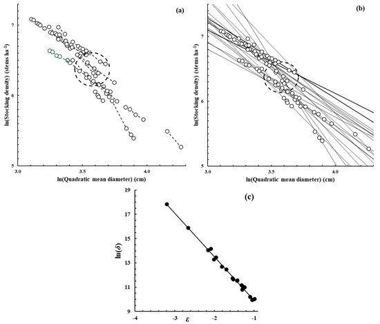
Figure 1.
Scatter plots (O) of the data available from each of the 20 E. obliqua plots that were available. In (a), the fine dashed lines (- - - -) join the data of each plot separately as the plot aged and its quadratic mean diameter increased and stocking density declined. In (b), the solid lines (––––) show the OLS regression fit to the data in each plot of Reineke’s dynamic thinning line (Function (3)); for each plot, its line has been extrapolated beyond the range of its data. In both (a,b), the elliptical shape (– – –) defines the 95% confidence region within which estimates of ln(N0) and ln(D0) lie as determined using the OLS fit of Model (8) to the data of these plots. In (c), a scatter plot (●) has been drawn between the estimates of parameters ln(δ) and ε from Function (3) for the 20 plots; the solid line (––––) is the OLS regression fit to the data of Model (8).
Table 1 lists the eight data sets that were available for the present work and their origins, together with some additional information about plot characteristics that was available for each species. Note that the data for Fagus sylvatica L. and Quercus petraea (Matt.) Liebl. had particularly wide spreads of stocking densities when compared with the other species. Both those data sets came from designed experimental trials that had unusually wide ranges of stocking densities at planting, 625–40,000 and 1333–500,000 stems ha−1, respectively.

Table 1.
Summary of the origins of the dynamic thinning line plot data used here for forests of various tree species around the world. The total number of plots for which data were included in each case is shown, together with the total number of measurements of those plots of which there were at least two for each plot. The minimum–mean–maximum ages of measurement of the plots of each species are shown where these could be determined. If shown in italics, the ages were not known directly but could only be determined approximately from information in the text of the corresponding publication.
3. Results
3.1. Dynamic Thinning Lines in E. obliqua Forest
Figure 1b shows a scatter plot of the dynamic data for each plot in the E. obliqua data set as each plot was self-thinning. The lines drawn there show the fit to the data of Reineke’s Function (3) for each plot; each of those lines have been extrapolated well beyond the range of the data from which they were determined. A scatter plot of the 20 sets of parameter estimates determined for Function (3) shows that they were highly correlated (Figure 1c); the correlation coefficient between them had a value of −0.997.
As discussed in the Introduction, various studies have found that the slopes and/or intercepts of the dynamic thinning lines of a set of plots, such as those here, may be related to the environmental circumstances of the plots; investigating that possibility was the initial objective of the present work. As described in Appendix A, no evidence was found here of such a relationship existing.
However, inspection by eye of Figure 1b suggested there was a tendency for the various dynamic thinning lines to intersect at a more or less common point, somewhere in the region of ln(N) ≈ 6.4 (N ≈ 602 stems ha−1) and ln(D) ≈ 3.6 (D ≈ 36.6 cm). Such a tendency was quite unexpected and does not seem to have been reported by others who have examined a set of dynamic thinning lines such as these. Suppose there is indeed a well-defined intersection region for such a set of dynamic thinning lines and its location is centered around some point ln(N0) and ln(D0). If it is assumed that Reineke’s Function (3) applies separately in each plot but passes through the common intersection point, then the dynamic thinning line for each plot might then be defined as having its origin at ln(N0) and ln(D0) and may be written as
where ε′ is a parameter. This can be rearranged as
which is equivalent to Reineke’s Function (3) but with
and
[ln(N) − ln(N0)] = ε′ [ln(D) − ln(D0)]
ln(N) = [ln(N0) − ε′ ln(D0)] + ε′ ln(D)
[ln(N0) − ε′ ln(D0)] ≡ ln(δ)
ε′ ≡ ε
Given this, the estimates of ln(δ) and ε obtained from the original fits of Function (3) for each plot (for the lines shown in Figure 1b in the present case) might be used to fit the linear model, rearranged from (6),
where ln(N0) and ln(D0) are treated as parameters. The estimates determined for ln(N0) and ln(D0) then define the mean of the intersection points of the lines. Estimates of the parameter standard errors from the regression analysis may then be used to define the confidence region within which the mean of the intersection points might lie.
ln(δ) = ln(N0) + ln(D0) [−ε]
For the present case, Model (8) was fitted using the data of ln(δ) and ε shown in Figure 1c, and the solid line shown there is the fit of the data from the OLS regression. The fitted model had a coefficient of determination (r2) of 0.994 and was highly significant (p < 0.001). It yielded estimates of ln(N0) = 6.372 (N0 = 585 stems ha−1), with a standard error of 0.112, and ln(D0) = 3.576 (D0 = 35.7 cm), with a standard error of 0.0647. Those estimates were close to the values mentioned above that were based simply on the visual inspection of Figure 1b. In Figure 1a,b, an elliptical shape was drawn, defining the 95% confidence region within which the estimates of ln(N0) and ln(D0) lie, as determined by this fitted model. That is to say, it appears that there is an approximately common intersection point within that region through which the dynamic thinning lines for the various plots tend to pass.
3.2. What Might Determine a Common Intersection Point?
The findings in the previous section led to the question as to whether or not a tendency for dynamic thinning lines to intersect at a common point is related to the level of correlation between the slopes and intercepts of the lines, as shown for E. obliqua in Figure 1c. This level of correlation determines the closeness of fit of Model (8) and hence the size of the confidence limit region within which the intersection point lies, as shown in Figure 1a,b.
A simulation study to examine this proposition was devised as follows. Figure 2 has the same form as Figure 1 but shows the data set used to initiate the simulation study. It was based on the E. obliqua data set using the original ln(D) data of each plot and the original slopes of the dynamic thinning line of each plot, as in Figure 1b. However, based on Model (5), the intercept of each line was then modified so that all the lines, when extrapolated, met at a common intersection point with ln(N) = 6.4 (N = 602 stems ha−1) and ln(D) = 3.6 (D = 36.6 cm), as evident in Figure 2b. Under those circumstances, the correlation between the ln(δ) and ε values of the lines was perfect, with a value of −1, as evident in Figure 2c. The ln(N) data of the original data set were then modified to conform to the new values of the intercepts of the dynamic thinning lines of each plot. This led to a revised data set, with a reduced spread between the plots, as evident by comparing Figure 1a and Figure 2a.
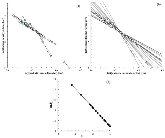
Figure 2.
Diagram with similar sections (a–c) and a similar form to that of Figure 1. It was based on the same E. obliqua data set but modified to become the initiation point of the simulation study described in the text.
The simulation study then proceeded as follows. Given the set of dynamic thinning line intercepts used to initiate the simulation (Figure 2b), an arbitrary variance was chosen and random normal deviates, with sizes based on that variance, were added to the intercepts. Model (8) was then applied to those data to yield estimates of ln(N0) and ln(D0) and their standard errors, hence confidence limits, exactly as described earlier for the original E. obliqua data set depicted in Figure 1. A new variance was then chosen and a new simulation carried out with the corresponding new set of intercepts. The larger the chosen variance, the larger the variation between the set of simulated intercepts and the smaller the level of correlation between the set of slopes and intercepts being used in the simulation.
As the level of correlation between the set of slopes and intercepts declined in any simulation, there was found to be a rapid increase in the size of the estimates of the confidence limits around the estimates of the mean values of ln(N0) and ln(D0). With a level of correlation close to that of the original data set, −0.997 (that of Figure 1c), the simulated 95% confidence interval of the estimate of ln(N0) ranged from 6.01 to 6.05 (the equivalent N0 range being 408−672 stems ha−1), whilst that of ln(D0) ranged from 3.56 to 3.58 (the equivalent D0 range being 35.2–47.0 cm). A reduction in the degree of correlation to only −0.960 led to a corresponding confidence interval for ln(N0) ranging from 4.83 to 6.85 (an equivalent N0 range of 126–943 stems ha−1) and ln(D0) ranging from 3.45 to 4.06 (equivalent D0 range of 31.4–100.1 cm). The latter range for the quadratic mean diameter of a forest stand of any tree species, grown even for some decades, had an upper limit of just over 100 cm, which is well above a level that is generally encountered and appears to be quite unrealistic in forest science terms.
These results suggest that, for the E. obliqua case studied here, there was indeed a tendency for the dynamic thinning lines of the various plots to intersect at points within a limited range of stocking densities and quadratic mean diameters, the 95% limits being defined by the ellipses in Figure 1a,b. These ranges would widen rapidly to biologically unrealistic limits with a reduction in the level of correlation between the set of slopes and intercepts of the dynamic thinning lines of the plots being considered.
3.3. Common Intersection Points for Other Species
The same methods as used for the data set of E. obliqua were applied to the data available for the other seven species under consideration here. The plot data and fitted dynamic thinning lines are shown in Figure A2a, Figure A3a, Figure A4a, Figure A5a, Figure A6a, Figure A7a and Figure A8a in Appendix B, as they were for E. obliqua in Figure 1b. The scatter plots of the estimates of parameters ln(δ) and ε from the dynamic lines are shown in Figure A2b, Figure A3b, Figure A4b, Figure A5b, Figure A6b, Figure A7b and Figure A8b. As for E. obliqua (Figure 1c), the correlations were very close in each case, as was the fit to the data of Model (8), which is shown as the solid line in each case. The results of fitting Model (8) are summarized in Table 2 (together with the results for E. obliqua). The levels of correlation shown there were highly significantly different from zero (p < 0.001 or less) in every case.

Table 2.
Results of fitting Model (8) to the data available for each of the eight species being considered here. The correlation coefficient shown is that between the estimates of parameters ln(δ) and ε of Function (3) for the set of plots for each species; its square is the coefficient of determination of the corresponding fit to the data of Model (8) for that species. The estimates of parameters ln(N0) and ln(D0) determined by fitting Model (8) are then shown, together (in parentheses) with the 95% confidence limits about those estimates.
The 95% confidence limits regarding the estimates from Model (8) of the common intersection points, ln(N0) and ln(D0), are shown in parentheses in Table 2; they have been plotted as ellipsoidal areas in the corresponding Figure A2a, Figure A3a, Figure A4a, Figure A5a, Figure A6a, Figure A7a and Figure A8a in Appendix B, as conducted for E. obliqua in Figure 1a,b. The unusually wide range of planting densities used in the experiments that yielded the Fagus sylvatica and Quercus petraea data (Figure A3 and Figure A4), as mentioned in Section 2, may have produced what appear to be the somewhat variable set of dynamic thinning lines in those cases; however, nothing in the fit to the data of Model (8) in those cases suggested they were behaving in any fashion that was different from that of the other species.
The results clearly suggest that there is a consistent tendency for the dynamic thinning lines of a set of plots in a monospecific population of a tree species to intersect at, and then pass through, a common intersection point. Attempts in this work to determine that point [ln(N0) and ln(D0)] for eight species from various parts of the world suggested that it was not exact for any one species, but it could be estimated to lie within a confidence region about some mean point. As can be determined from Table 2, the widths of those 95% confidence regions for ln(N0) varied from 3 to 14% of the corresponding estimate of their means and from 3 to 16% for ln(D0). The sizes of the corresponding ellipsoidal confidence regions can appear very different when plotted on graphs (Figure 1, Figure A2, Figure A3, Figure A4, Figure A5, Figure A6, Figure A7 and Figure A8). However, this can be somewhat misleading as the sizes reflect the scales to which the diagrams are drawn and the ranges that the data encompass.
4. Discussion
At the outset of this work, it had been intended to examine if a set of dynamic thinning lines, determined using data from a set of forest plots of E. obliqua from Tasmania, Australia, differed in their slopes and/or intercepts due to differences in site productive capacity. Using stand site index as the measure of productive capacity, that did not seem to be the case (Figure A1, Appendix A). As mentioned in the Introduction, others have found that some species show effects of site productive capacity whilst others do not.
As the work continued with the E. obliqua data set, it appeared that, if the dynamic thinning lines of the various plots were extrapolated, they tended to all intersect in the vicinity of a single point (Figure 1b) at a stand stocking density of about 585 stems ha−1 and a quadratic mean diameter near 35.7 cm. A method was devised to use regression analysis to estimate the position of the intersection point and a confidence limit of the region in which the point lies (Model 8). That region is shown for the E. obliqua data set in Figure 1a,b.
The authors of the present work were unable to find previous reports of this phenomenon for any forest species. An initial reaction to it here was that it might be inevitable. After all, any pair of non-parallel straight lines must intersect at some point; perhaps the structure of the data being used here ensured that would be the case. A simple simulation exercise was devised to examine the matter. It started from a simulated data set where all the lines intersected exactly at one point (Figure 2b). As the intercepts of the lines were altered randomly, the common intersection point was soon lost. However, it was clear that the degree of correlation between the slopes and intercepts of the lines was closely related to the presence or absence of the common intersection point. For the E. obliqua case, that correlation coefficient was indeed high at −0.997 (Figure 1c).
Data similar in form to those for E. obliqua were then obtained from the literature for monospecific forests of seven other species, five hardwood and two softwood, from populations scattered widely across the world (Table 1). In each case, the correlations between the slopes and intercepts of their set of dynamic thinning lines were high (Table 2), with the widths of their 95% confidence limits all lying within 3–16% of the estimated positions of both the stocking densities and quadratic mean diameters of the intersection points (or at least their natural logarithms). The data and results for all seven species are shown in Figure A2, Figure A3, Figure A4, Figure A5, Figure A6, Figure A7 and Figure A8 in Appendix B. It was concluded that it seemed generally true that the dynamic thinning lines of a set of plots from monospecific forests of a tree species tended to intersect at an approximately common intersection point.
The finding of this common intersection point of dynamic thinning lines does not have any consequence for the principles of the self-thinning rule. This can be appreciated through Equation (4), which defines the dynamic thinning line as it passes through a particular point with stocking density N0 and quadratic mean diameter D0. It can be rewritten as
and, hence,
This is completely equivalent to Reineke’s Function (3) but with
and
Thus, Yoda et al.’s [1] original concept of the self-thinning rule is completely supported even with this constraint that dynamic thinning lines from many stands pass through, or near, a common intersection point. However, this new phenomenon does add an additional concept to the rule, expressed here through Equations (10)–(12).
N = N0 (D/D0)ε′
N = δ′Dε′.
δ’ = N0/(D0)ε′
ε′ = ε.
At present, it is possible only to speculate as to what aspects of the biology of tree growth behavior might lead to the occurrence of this phenomenon. As a stand grows, the average size of the trees that remain alive within it at any time increases. However, the rate of increase in this average size declines with time because of a decline with increasing age in overall stand growth rates (5—Section. 8.10, [55,56,57]–Chap. 4, [58,59,60,61]), probably due to increased respiratory demands with increasing age [62] and due to losses of trees through mortality. At the same time as live tree sizes increase, their need for the resources from the site each requires for growth (light, water, and mineral nutrients) increases. On any particular site, the availability of those resources is limited and the trees must compete with each other for access to them. Because of their larger sizes, larger trees have greater competitive ability than smaller trees. Eventually, the growth of smaller trees is suppressed and it is they that tend to die, leading to changes with time in stocking density and average tree size that then conform to the self-thinning rule. The presence of a common intersection point of dynamic thinning lines in a tree population suggests there must be some balance between tree growth behavior and competitive interactions between trees and how these determine mortality amongst smaller trees. Exactly how and why such a balance occurs is unknown at present.
Certainly, for any species, there was some variation around the average point where the dynamic thinning lines intersected. This variation was reflected in a confidence limit showing variation about their average intersection point (Table 2 and Figure 1, Figure A2, Figure A3, Figure A4, Figure A5, Figure A6, Figure A7 and Figure A8). Again, no immediate explanation exists to explain this variation. Perhaps it reflects variations in growth behavior as a consequence of the different environmental circumstances under which plots grow, or differences in the original planting or regeneration densities of plots, or the timing of different management practices such as thinning. Perhaps, as these effects become greater, they may overtake the inferred growth–competition–mortality balances mentioned above and remove the tendency for a common intersection.
5. Conclusions
The unexpected conclusion from this work was that there is a tendency for a set of dynamic thinning lines in even-aged monospecific forest plots to intersect near a common point. The data for nine species, both hardwood and softwood from around the world, supported this conclusion. This phenomenon adds a new element to the concept of the self-thinning rule without altering the principles of the rule (Equations (10)–(12)).
This phenomenon does not seem to have been observed before. It may be a consequence of growth patterns, inter-tree competitive processes, and patterns of mortality interacting to lead to the common stand circumstances. The initial work to examine the forest growth behavior characteristics that explain the phenomenon might explore many existing forest growth models to determine if any of them predict it. If so, such models may lead to suggestions as to what mechanisms determine it. If none does, it will suggest that new work is necessary to both understand the phenomenon and develop growth models that predict its occurrence.
Author Contributions
Investigation, P.W.W. and D.A.R.; Writing—original draft, P.W.W.; Writing—review & editing, D.A.R. All authors have read and agreed to the published version of the manuscript.
Funding
The authors received no funding for this work.
Data Availability Statement
The E. obliqua data used in this study are available on request from the corresponding author.
Conflicts of Interest
The authors declare no conflict of interest.
Appendix A. Site Index Effects in E. obliqua
In the present case, the site index of each plot was known, and it was considered that it might reflect the environmental circumstances of each plot. Figure A1 shows a scatter plot of the parameter estimates of Function (3) against plot site index. Inspection of the figure suggests that there was no appreciable relationship present. In both cases, the correlation coefficient between the parameter estimates and site index was <0.3 and did not differ significantly from zero (p = 0.05). Because of the high level of correlation between ln(δ) and ε (Figure 1c), the scatter plots of Figure A1a,b are virtual mirror images of each other if reflected across the site index axis.
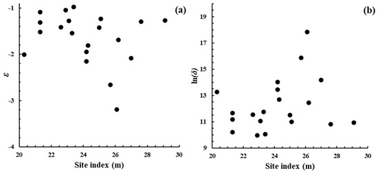
Figure A1.
Scatter plots of the parameters estimated for the dynamic thinning lines [Function (3)] of the 20 E. obliqua plots available here against the site index of each plot.
Appendix B. Dynamic Thinning Lines of Other Species
Figure A2, Figure A3, Figure A4, Figure A5, Figure A6, Figure A7 and Figure A8 were constructed in a similar fashion to Figure 1b,c in the main text for E. obliqua. They are for monospecific forest data sets of seven other species, as listed in Table 1 and Table 2. The origins of the data are shown in each case. In (a), each data set consisted of at least two measurements (O) taken from each of several plots that had reached their dynamic thinning line. The elliptical shape (– – –) defines the 95% confidence region within which lay estimates of ln(N0) and ln(D0). In (b), the scatter plot (●) was between the estimates of parameters ln(δ) and ε from Function (3) for the plots concerned.
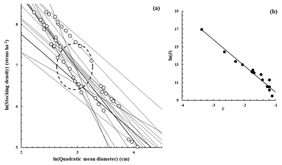
Figure A2.
Eucalyptus camaldulensis Denh.—[51], Supplementary data from the publication.
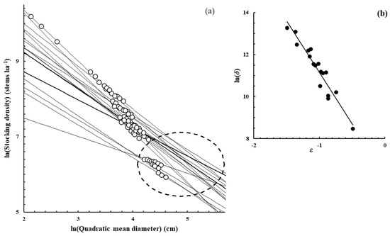
Figure A3.
Fagus sylvatica L.—[22,52], Supplementary data from the publication.
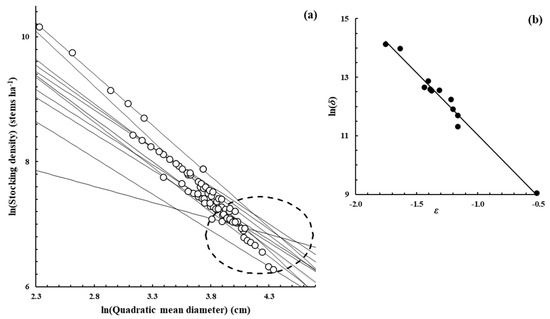
Figure A4.
Quercus petraea (Matt.) Liebl.—[22], Supplementary data from the publication.
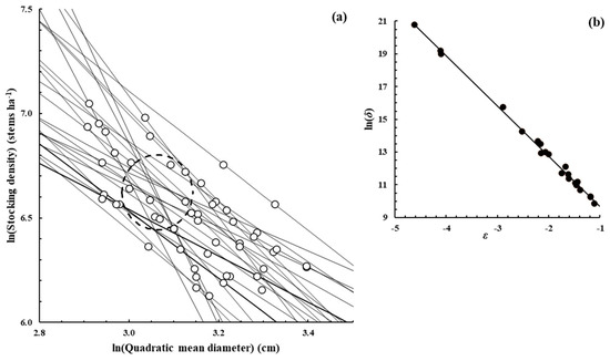
Figure A5.
Populus tremuloides Michx.—[37], Measured from the publication Figure 4A.
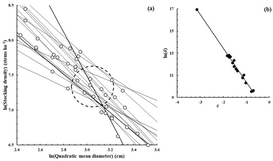
Figure A6.
Nothofagus spp.—[53], Measured from the publication Figure 2.
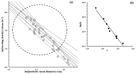
Figure A7.
Pinus pinaster Aiton.—[8], Measured from the publication Figure 3b.
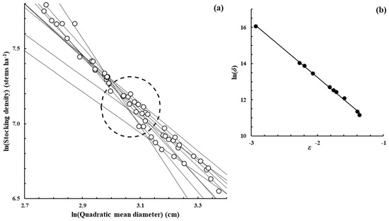
Figure A8.
Pinus taeda L.—[54], Measured from the publication Figure 4.
References
- Yoda, K.; Kira, T.; Ogawa, H.; Hozumi, K. Self-thinning in overcrowded pure stands under cultivated and natural conditions. J. Biol. Osaka City Univ. 1963, 14, 107–129. [Google Scholar]
- Gorham, E. Shoot height, weight and standing crop in relation to density of monospecific stands. Nature 1979, 279, 148–150. [Google Scholar] [CrossRef]
- White, J. The allometric interpretation of the self-thinning rule. J. Theor. Biol. 1981, 89, 475–500. [Google Scholar] [CrossRef]
- Reineke, L.H. Perfecting a stand-density index for even-aged forests. J. Agric. Res. 1933, 46, 627–638. [Google Scholar]
- West, P.W. Tree and Forest Measurement, 3rd ed.; Springer International Publishing: Cham, Switzerland, 2015. [Google Scholar]
- Weller, D.E. Will the real self-thinning rule stand up?—A reply to Osawa and Sugita. Ecology 1990, 71, 1204–1207. [Google Scholar] [CrossRef]
- VanderSchaaf, C.L.; Burkhart, H.E. Comparison of methods to estimate Reineke’s maximum size-density relationship species boundary line slope. For. Sci. 2007, 53, 435–442. [Google Scholar] [CrossRef]
- Pavel, M.A.A.; Barreiro, S.; Tomé, M. The importance of using permanent plots data to fit the self-thinning line: An example for maritime pine stands in Portugal. Forests 2023, 14, 1354. [Google Scholar] [CrossRef]
- Caicoya, A.T.; Biber, P.; del Rio, M.; Ruiz-Peinado, R.; Arcangeli, C.; Matthews, R.; Pretzsch, H. Self-thinning of Scots pine across Europe changes with solar radiation, precipitation and temperature but does not show trends in time. For. Ecol. Manag. 2024, 552, 121585. [Google Scholar]
- Puettmann, K.J.; Hann, D.W.; Hibbs, D.E. Evaluation of the size-density relationships for pure red alder and Douglas-fir stands. For. Sci. 1993, 39, 7–27. [Google Scholar] [CrossRef]
- Pretzsch, H.; Biber, P. A re-evaluation of Reineke’s rule and stand density index. For. Sci. 2005, 51, 304–320. [Google Scholar] [CrossRef]
- de Montigny, L.; Nigh, G. Density frontiers for even-aged Douglas-fir and western hemlock stands in coastal British Columbia. For. Sci. 2007, 53, 675–682. [Google Scholar] [CrossRef]
- Comeau, P.G.; White, M.; Kerr, G.; Hale, S.E. Maximum density-size relationships for Sitka spruce and coastal Douglas-fir in Britain and Canada. Forestry 2010, 83, 461–468. [Google Scholar] [CrossRef]
- Charru, M.; Seynave, I.; Morneau, F.; Rivoire, M.; Bontemps, J.-D. Significant differences and curvilinearity in the self-thinning relationships of 11 temperate tree species assessed from forest inventory data. Ann. For. Sci. 2012, 69, 195–205. [Google Scholar] [CrossRef]
- Brunet-Navarro, P.; Sterck, F.J.; Vayreda, J.; Martinez-Vilalta, J.; Mohren, G.M.J. Self-thinning in four pine species: An evaluation of potential climate impacts. Ann. For. Sci. 2016, 73, 1025–1034. [Google Scholar] [CrossRef]
- Riofrío, J.; del Río, M.; Bravo, F. Mixing effects on growth efficiency in mixed pine forests. Forestry 2016, 90, 381–392. [Google Scholar] [CrossRef]
- Condés, S.; Vallet, P.; Bielak, K.; Bravo-Oviedo, A.; Voll, L.; Ducey, M.J.; Pach, M.; Pretzsch, H.; Sterba, H.; Vayreda, J.; et al. Climate influences on the maximum size-density relationship in Scots pine (Pinus sylvestris L.) and European beech (Fagus sylvatica L.) stands. For. Ecol. Manag. 2017, 385, 295–307. [Google Scholar] [CrossRef]
- Aguirre, A.; del Rio, M.; Condes, S. Intra- and inter-specific variation of the maximum size-density relationship along an aridity gradient in Iberian pinewoods. For. Ecol. Manag. 2018, 411, 90–100. [Google Scholar] [CrossRef]
- Quiñonez-Barraza, G.; Tamarit-Urias, J.C.; Martínez-Salvador, M.; García-Cuevas, X.; Santos-Posadas, H.M.; Santiago-García, W. Maximum density and density management diagram for mixed-species forests in Durango, Mexico. Revista Chapingo Serie Ciencias Forestales y del Ambiente 2018, 24, 73–90. [Google Scholar] [CrossRef]
- Lee, D.; Choi, J. Evaluating maximum stand density and size-density relationships based on the Competition Density Rule in Korean pines and Japanese larch. For. Ecol. Manag. 2019, 446, 204–213. [Google Scholar] [CrossRef]
- Pretzsch, H. The effect of tree crown allometry on community dynamics in mixed-species stands versus monocultures. A review and perspectives for modeling and silvicultural regulation. Forests 2019, 10, 810. [Google Scholar] [CrossRef]
- Ningre, F.; Ottorini, J.-M.; Le Goff, N. Modeling size-density trajectories for even-aged oak (Quercus petraea Liebl.) stands and comparison with beech (Fagus silvatica L.) in France. Ann. For. Sci. 2019, 76, 73. [Google Scholar] [CrossRef]
- de Prado, D.R.; San Martín, R.; Bravo, F.; de Aza, C.H. Potential climatic influence on maximum stand carrying capacity for 15 Mediterranean coniferous and broadleaf species. For. Ecol. Manag. 2020, 460, 117824. [Google Scholar] [CrossRef]
- Donald, C.M. Competition among pasture plants. I. Interspecific competition among annual pasture plants. Aust. J. Agric. Res. 1951, 2, 355–376. [Google Scholar] [CrossRef]
- Shinozaki, K.; Kira, T. Intraspecific competition among higher plants VII. Logistic theory of the C-D effect. J. Inst. Polytech. 1956, 12, 69–82. [Google Scholar]
- Tang, S.; Meng, F.-R.; Meng, C.H. The impact of initial stand density and site index on maximum density index and self-thinning index in a stand self-thinning model. For. Ecol. Manag. 1995, 75, 61–68. [Google Scholar] [CrossRef]
- Bi, H.Q. The self-thinning surface. For. Sci. 2001, 47, 361–370. [Google Scholar] [CrossRef]
- Bi, H.Q. Stochastic frontier analysis of a classic self-thinning experiment. Austral Ecol. 2004, 29, 408–417. [Google Scholar] [CrossRef]
- Pittman, S.D.; Turnblom, E.C. A study of self-thinning using coupled allometric equations: Implications for coastal Douglas-fir stand dynamics. Can. J. For. Res. 2003, 33, 1661–1669. [Google Scholar] [CrossRef]
- Poage, N.J.; Marshall, D.D.; McClellan, M.H. Maximum stand-density index of 40 western hemlock–Sitka spruce stands in southeast Alaska. Western J. App. For. 2007, 22, 99–104. [Google Scholar] [CrossRef]
- Weiskittel, A.; Gould, P.; Temesgen, H. Sources of variation in the self-thinning boundary line for three species with varying levels of shade tolerance. For. Sci. 2009, 55, 84–93. [Google Scholar] [CrossRef]
- Schütz, J.P.; Zingg, A. Improving estimations of maximal stand density by combining Reineke’s size-density rule and the yield level, using the example of spruce (Picea abies (L.) Karst.) and European Beech (Fagus sylvatica L.). Ann. For. Sci. 2010, 67, 507. [Google Scholar] [CrossRef]
- Reyes-Hernandez, V.; Comeau, P.G.; Bokalo, M. Static and dynamic maximum size-density relationships for mixed trembling aspen and white spruce stands in western Canada. For. Ecol. Manag. 2013, 289, 300–311. [Google Scholar] [CrossRef]
- Zhang, J.W.; Oliver, W.W.; Powers, R.F. Reevaluating the self-thinning boundary line for ponderosa pine (Pinus ponderosa) forests. Can. J. For. Res. 2013, 43, 963–971.9604. [Google Scholar] [CrossRef]
- Zhang, X.; Cao, Q.V.; Duan, A.; Zhan, G.J. Self-thinning trajectories of Chinese fir plantations in Southern China. For. Sci. 2016, 62, 594–599. [Google Scholar] [CrossRef]
- Zhang, X.Q.; Lu, L.L.; Cao, Q.V.; Duan, A.G.; Zhang, J.G. Climate-sensitive self-thinning trajectories of Chinese fir plantations in south China. Can. J. For. Res. 2018, 48, 1388–1397. [Google Scholar] [CrossRef]
- Kweon, D.; Comeau, P.G. Effects of climate on maximum size-density relationships in Western Canadian trembling aspen stands. For. Ecol. Manag. 2017, 406, 281–289. [Google Scholar] [CrossRef]
- Forrester, D.I.; Baker, T.G.; Elms, S.R.; Hobi, M.L.; Ouyang, S.; Wiedmann, J.C.; Xiang, W.; Zell, J.; Pulkkinen, M. Self-thinning tree mortality models that account for vertical stand structure, species mixing and climate. For. Ecol. Manag. 2021, 487, 118936. [Google Scholar] [CrossRef]
- Le Goff, N.; Ningre, F.; Ottorini, J.M. Modeling size-density trajectories of even-aged ash (Fraxinus excelsior L.) stands in France. A baseline to assess the impact of Chalara ash dieback. Ann. For. Sci. 2021, 78, 3. [Google Scholar] [CrossRef]
- Marqués, L.; Weng, E.; Bugmann, H.; Forrester, D.I.; Rohner, B.; Hobi, M.L.; Trotsiuk, V.; Stocker, B.D. Tree growth enhancement drives a persistent biomass gain in unmanaged temperate forest. AGU Adv. 2023, 4, e2022AV000859. [Google Scholar] [CrossRef]
- Dong, L.B.; Chen, G.M.; Chung, W.; Liu, Z.G. Variations on the maximum density-size lines to climate and site factors for Larix spp. plantations in northeast China. Ecol. Model. 2024, 498, 110913. [Google Scholar] [CrossRef]
- Lee, D.; Siipilehto, J.; Hynynen, J. Comparison and analysis of self-thinning models based on diameter-based maximum size-density relationships. For. Ecol. Manag. 2025, 575, 122374. [Google Scholar] [CrossRef]
- Mrad, A.; Manzoni, S.; Oren, R.; Vico, G.; Lindh, M.; and Katul, G. Recovering the metabolic self-thinning, and constant final yield rules in mono-specific stands. Front. For. Glob. Chang. 2020, 3, 62. [Google Scholar] [CrossRef]
- Avery, T.E.; Burkhart, H.E. Forest Measurements, 5th ed.; McGraw Hill: New York, NY, USA, 2002. [Google Scholar]
- Burkhart, H.E. Comparison of maximum size-density relationships based on alternate stand attributes for predicting tree numbers and stand growth. For. Ecol. Manag. 2013, 289, 404–408. [Google Scholar] [CrossRef]
- Mattay, J.P.; West, P.W. A Collection of Growth and Yield Data from Eight Eucalypt Species Growing in Even-Aged, Monoculture Forest. CSIRO Division of Forestry, User Series No 18; Canberra. 1994. Available online: http://sciwest.byethost6.com/Mattay&West1994EucalyptdataCSIRO.pdf (accessed on 15 December 2024).
- West, P.W.; Mattay, J.P. Yield prediction models and comparative growth rates for six eucalypt species. Aust. For. 1993, 56, 211–225. [Google Scholar] [CrossRef]
- Bacon, D.W.; Watts, D.G. Estimating the transition between two intersecting straight lines. Biometrika 1971, 58, 525–534. [Google Scholar] [CrossRef]
- Deleuze, C.; Pain, O.; Dhôte, J.-F.; Hervé, J.-C. A flexible radial increment model for individual trees in pure even-aged stands. Ann. For. Sci. 2004, 61, 327–335. [Google Scholar] [CrossRef][Green Version]
- West, P.W.; Ratkowsky, D.A. Models relating individual tree basal area growth rates to tree basal areas in even-aged, monoculture forest stands. J. For. 2022, 9, 21–38. [Google Scholar] [CrossRef]
- Trouvé, R.; Nitschke, C.R.; Robinson, A.P.; Baker, P.J. Estimating the self-thinning line from mortality data. For. Ecol. Manag. 2017, 402, 122–134. [Google Scholar] [CrossRef]
- Ningre, F.; Ottorini, J.-M.; Le Goff, N. Modelling size-density trajectories for even-aged beech (Fagus sylvatica L.) stands in France. Ann. For. Sci 2016, 73, 765–776. [Google Scholar] [CrossRef]
- Salas-Eljatib, C.; Weiskittel, A.R. Evaluation of modeling strategies for assessing self-thinning behavior and carrying capacity. Ecol. Evol. 2018, 8, 10768–10779. [Google Scholar] [CrossRef]
- VanderSchaaf, C.L. Estimating individual stand size-density trajectories and a maximum size-density relationship species boundary line slope. For. Sci. 2010, 56, 327–335. [Google Scholar] [CrossRef]
- Gower, S.T.; McMurtrie, R.E.; Murty, D. Aboveground net primary production decline with stand age: Potential causes. Trends Ecol. Evol. 1996, 11, 378–382. [Google Scholar] [CrossRef] [PubMed]
- Ryan, M.G.; Binkley, D.; Fownes, J.H. Age-related decline in forest productivity: Pattern and process. Adv. Ecol. Res. 1997, 27, 213–262. [Google Scholar]
- Davis, L.S.; Johnson, K.N.; Bettinger, P.S.; Howard, T.E. Forest Management, 4th ed.; McGraw-Hill: New York, NY, USA, 2001. [Google Scholar]
- Skovsgaard, J.P.; Vanclay, J.K. Forest site productivity: A review of spatial and temporal variability in natural site conditions. Forestry 2013, 86, 305–315. [Google Scholar] [CrossRef]
- Binkley, D. Acorn review: The persistent mystery of declining growth in older forests. For. Ecol. Manag. 2023, 538, 121004. [Google Scholar] [CrossRef]
- Pretzsch, H.; del Rio, M.; Arcangeli, C.; Bielak, K.; Dudzinska, M.; Forrester, D.I.; Kohnle, U.; Ledermann, T.; Matthews, R.; Nagel, R.; et al. Competition-based mortality and tree losses. An essential component of net primary productivity. For. Ecol. Manag. 2023, 544, 21204. [Google Scholar] [CrossRef]
- West, P.W. A review of the growth behaviour of stands and trees in even-aged, monospecific forest. Ann. For. Sci. 2024, 81, 34. [Google Scholar] [CrossRef]
- West, P.W. Do increasing respiratory costs explain the decline with age in forest growth rate? J. For. Res. 2020, 31, 693–712. [Google Scholar] [CrossRef]
Disclaimer/Publisher’s Note: The statements, opinions and data contained in all publications are solely those of the individual author(s) and contributor(s) and not of MDPI and/or the editor(s). MDPI and/or the editor(s) disclaim responsibility for any injury to people or property resulting from any ideas, methods, instructions or products referred to in the content. |
© 2025 by the authors. Licensee MDPI, Basel, Switzerland. This article is an open access article distributed under the terms and conditions of the Creative Commons Attribution (CC BY) license (https://creativecommons.org/licenses/by/4.0/).