1. Introduction
Climate change poses serious challenges to forest ecosystems worldwide, where drought has become one of the leading causes of forest decline [
1]. Drought stress impairs plant physiology by limiting photosynthesis, nutrient uptake, and growth. These effects can reduce productivity, alter canopy structure, and reshape species composition [
2]. Accurate and timely evaluation of tree water status is critical for climate-smart forestry. Traditional approaches, mainly manual field surveys or single-sensor remote sensing [
3], lack the capacity to capture the subtle and early physiological and structural responses of trees to water deficit at a fine scale. As a result, there is a pressing demand to develop advanced tools and technologies that improve the efficiency and precision of forest health monitoring and stress diagnosis.
This need is a primary driver behind the rise in high-throughput plant phenotyping technology [
4]. These systems integrate automation with sophisticated sensor arrays—including RGB, hyperspectral, thermal, and LiDAR sensors [
5,
6]. Although it originated in agricultural research, it has also shown great potential in forestry research, providing a new perspective for non-destructive and quantitative analysis of plant structure and function [
7]. For example, Cohen used drone thermal imaging technology to map the changes in water conditions in
date palm forests to customize irrigation plans [
8]. Saarinen used hyperspectral cameras combined with radar point clouds to obtain the volume of deciduous trees in forest blocks to assess forest health [
9]. Accurate analysis of forest phenotypic traits is essential for understanding how plant’s genes, phenotypes, and environmental factors interact under climate change [
10,
11,
12]. Such analysis underpins the advancement of smart forestry technologies. Phenotyping platforms can be categorized into two types: field-based and indoor systems. Field platforms, such as vehicle-mounted or drone systems, can provide valuable spatial environmental information. They are influenced by environmental variables and face challenges in data standardization and result reproducibility [
13,
14]. However, despite progress in field-based remote sensing, controlled indoor systems remain essential for isolating the physiological drivers of drought responses and for validating multimodal fusion methods under repeatable condition. In contrast, indoor phenotyping systems offer significant advantages through precise environmental control. They provide an ideal environment for systematically analyzing plant physiological responses to specific stresses, such as drought, and for establishing robust diagnostic models. This controlled setting effectively reduces the impact of confounding factors. Examples of such platforms include LemnaTec’s Scanalyzer HTC (Germany) and Crop3D from the Chinese Academy of Sciences’ Institute of Botany [
15]. Consequently, indoor platforms play a vital role in developing and validating multi-sensor data fusion techniques and serve as testbeds for future smart forestry monitoring systems.
Single-sensor techniques can detect drought-induced physiological changes to some extent, but each modality has its limitations. Thermal infrared imaging can track canopy temperature variations, yet, its performance is strongly influenced by the background temperature, wind speed, solar radiation, and canopy structure [
16,
17]. Hyperspectral imaging can capture subtle biochemical changes related to water absorption features, although its performance often decreases when spectral responses saturate under severe stress [
18]. Physiological and structural changes in plants are tightly linked and unfold across different spatial and temporal scales. Under complex stress conditions such as drought, these processes often occur asynchronously, making them challenging to capture with a single sensor [
19]. Multi-sensor data fusion has been a promising method to address this limitation by combining complementary information from different sources. Sankaran‘s research showed that combining hyperspectral and thermal imaging can improve drought prediction accuracy by integrating biochemical and thermal responses [
20]. Zhu reported that hyperspectral–LiDAR fusion can enhance assessments of canopy water content and structural changes in forests [
21]. Nonetheless, effectively integrating heterogeneous data with varying resolutions and physical properties presents challenges in registration, feature alignment, and biological interpretation [
22]. Therefore, establishing a reliable multimodal analysis framework to resolve these issues is an important step toward improving forest monitoring.
To overcome these limitations, we designed a three-axis gantry platform with high positional precision. This integrated system enables synchronized operation of a hyperspectral camera, a thermal infrared imager, and a LiDAR sensor to acquire complementary physiological and structural data of plants. The platform supports a multimodal data processing framework that extracts features indicative of plant water stress. The framework first applies sensor-specific image processing techniques to obtain relevant features. Next, a multi-kernel extreme learning machine (WOA-MK-ELM) model, optimized using the whale swarm algorithm, is constructed. This model adaptively fuses hyperspectral and thermal features through a double Gaussian kernel, enabling precise classification of water stress levels. Experimental results demonstrate that the hybrid model achieves classification accuracy notably higher than that of single-sensor models.
Early detection of drought-induced water stress is crucial for maintaining forest health. Integrated complementary sensing modalities should improve the early and reliable detection of water stress in forest seedlings compared with single-sensor methods. The aim of this study is to develop and validate a multi-sensor monitoring framework that can support intelligent forestry applications. To meet this objective, we designed an indoor phenotyping acquisition system capable of synchronously collecting multi-sensors data, allowing us to evaluate how multimodal information enhances the characterization of water stress responses relevant to forestry research. This study focuses on three main objectives:
- (1)
Developing a prototype multi-sensor acquisition system as a controlled platform for evaluating multimodal water stress indicators;
- (2)
Establishing a unified multimodal data processing pipeline to extract physiological and structural traits related to water stress from heterogeneous sensor data;
- (3)
Constructing a hybrid machine learning framework to adaptively integrate multimodal features for early drought-stress analysis.
2. Materials and Methods
2.1. Design of Experiment
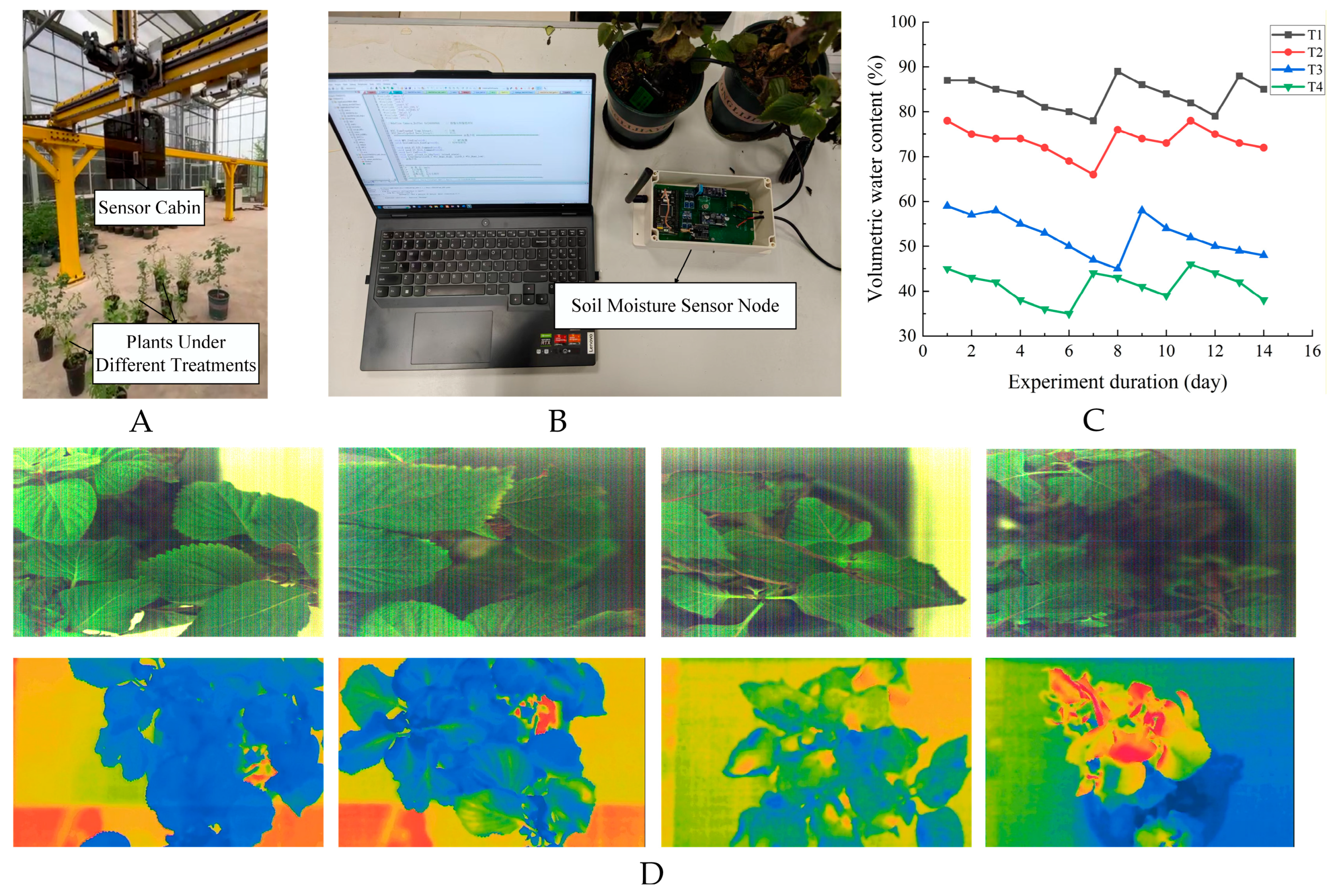
To evaluate whether our multimodal sensing method can improve the detection of plant water stress, we established a controlled indoor phenotyping platform in the greenhouse of XiaShu Forest Farm of Nanjing Forestry University (
Figure 1A). The platform integrates hyperspectral imaging, thermal infrared imaging, and LiDAR-based structural sensing to capture complementary physiological and morphological responses to drought. A controlled greenhouse experiment was designed to systematically test how these multimodal measurements respond to different levels of water deficit. The experiment provides a validation framework for assessing the feasibility of multi-sensor phenotyping approaches before extending them to more complex forest environments.
We selected
Perilla frutescens as the model plant for water-stress validation for three reasons: (1) Herbaceous and woody plants share similar physiological mechanisms in response to drought stress, including stomatal regulation, water balance adjustment, pigment changes, and reactive oxygen species (ROS) metabolism. These similarities have been confirmed by comparative physiology studies across both plant types [
23]. (2)
Perilla shows clear and quantifiable responses under water stress. Its canopy structure and leaf surface properties monitored with high sensitivity that are well suited for evaluating imaging-based drought indicators. This feature also emphasized in other sensor phenotyping studies [
24]. (3) Drought indicators based on imaging sensors have cross-species applicability. Previous work has demonstrated that physiological and imaging-derived stress indicators established in herbaceous species can inform drought responses in woody plants. For instance, Munns showed that stress signatures identified in herb experiments could be interpreted in woody plants [
25]. Sims & Gamon proposed that reflectance indices such as PRI and WI retain sensitivity across a wide range of species [
26].
To investigate how our multimodal sensors respond to different water-availability conditions, we imposed four irrigation treatments—waterlogging stress (T1), normal irrigation (T2), mild drought (T3), and severe drought (T4)—which correspond to stress levels I–IV. Rather than applying fixed watering blindly, we delivered quantitatively controlled irrigation volumes and simultaneously tracked soil relative water content (RWC) using a soil moisture sensor (Shandong Vemsee Technology Co., Ltd., Weifang, China). We monitored RWC daily and adjusted irrigation accordingly, and we maintained stable and clearly differentiated moisture levels for each stress treatment. The use of sensor and results are displayed in
Figure 1B,C. This approach allowed us to reliably simulate four well-defined water stress gradients, similar to strategies widely used in controlled plant phenotyping studies [
27].
Multi-source plant phenotyping data were collected in three acquisition phases to guarantee adequate sample size and stable coverage of the four water-stress treatments. The first two phases ran from 15 to 24 April 2025, and from 5 to 14 June 2025, following a twice-daily imaging schedule (9:30–10:30 a.m. and 2:30–3:30 p.m.) with two acquisition cycles per session.
To further strengthen the robustness of the dataset and address variability across plant growth stages, an additional acquisition phase was carried out from 3 to 12 September 2025, using the same greenhouse setup, sensor configuration, and irrigation treatments (T1–T4). This extension increased the number of multimodal datasets from the initial 240 to a total of 720 samples.
Figure 1D shows some of this data, corresponding to stress degree I to IV from left to right.
2.2. Design of the Multi-Sensor Prototype Platform
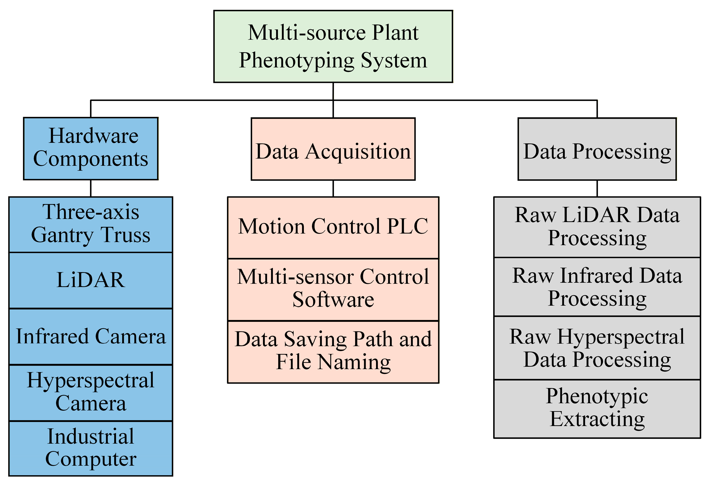
To support synchronized multimodal acquisition for water stress analysis, we developed a custom phenotyping prototype consisting of three modules: hardware architecture, control and synchronization, and a data-processing pipeline (
Figure 2). Its design builds on concepts from commercial platforms such as the LemnaTec Scanalyzer and Crop3D systems, which have been widely used for controlled-environment phenotyping of agricultural crops. The Scanalyzer series provides pre-configured RGB, fluorescence, or hyperspectral imaging with fixed mounting geometries suited to small herbaceous plants [
28], whereas Crop3D employs a gantry-based RGB–depth configuration with limited Z-axis travel and restricted compatibility with additional modalities such as LiDAR or high-resolution hyperspectral sensors [
29]. These systems also frequently rely on independent or software-level triggering, which may introduce temporal offsets that complicate multimodal fusion, particularly when combining sensors with heterogeneous frame rates [
30].
To tackle these issues, our prototype was specifically built for forestry phenotyping, where woody seedlings have greater canopy complexity and demand larger working volumes, stable scanning, and repeatable sensor positioning. A modular design was adopted to enable flexible integration of heterogeneous sensors and mechanically robust alignment within a unified cabin structure. In addition, a unified software-level triggering protocol and a multi-sensor calibration workflow were implemented to minimize temporal drift and geometric inconsistencies. Together, these procedures ensure stable, time-aligned, and spatially consistent multimodal acquisition suitable for downstream feature-level fusion in water stress analysis.
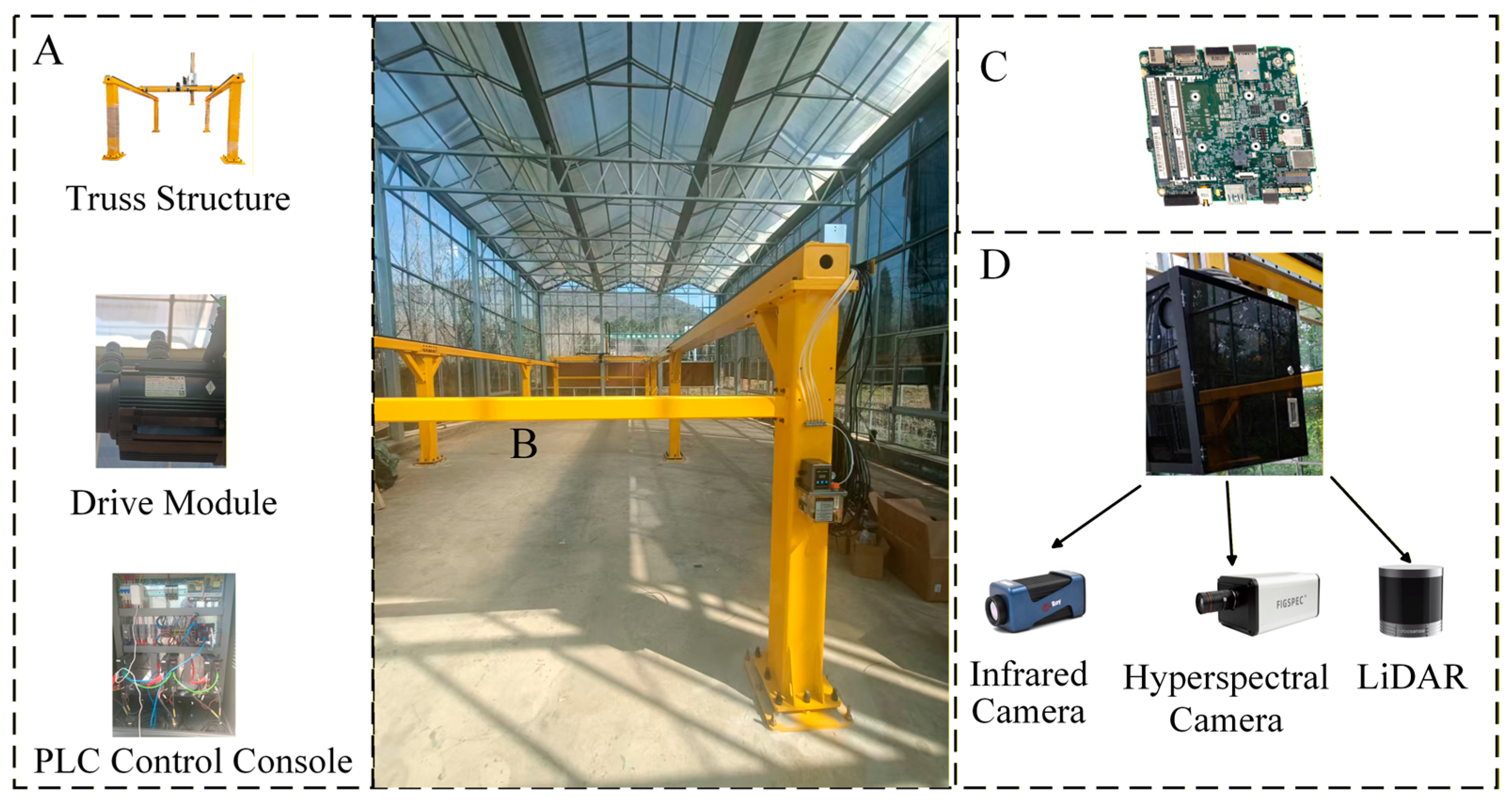
The phenotyping platform’s hardware architecture comprises four main components, with photographs of each presented in
Figure 3. Their functions are described as follows:
- (1)
The core framework of the indoor high-throughput phenotyping platform comprises Parts A and B, built around a commercial three-axis gantry system (Shenzhen Litai Automation Co., Ltd., Shenzhen, China). It owns high positional repeatability and the ability to carry the multiple optical sensors. While many commercial indoor phenotyping systems, such as LemnaTec Scanalyzer and Crop3D, are primarily designed for agricultural crops, their working volumes and sensor configurations may not fully accommodate the structural characteristics of woody seedlings or tree saplings. To address these requirements, we designed a modular sensor cabin mounted on the Z-axis of the gantry. It can adjust imaging height and stable operation during slow scanning, thus enabling simultaneous acquisition of thermal, hyperspectral, and LiDAR data. The gantry spans 18 m (X-axis), 4 m (Y-axis), and 2.1 m (Z-axis), providing a sufficiently large working volume for phenotyping. A PLC-based motion control system directs the movement of each axis, which allows accurate positioning and smooth motion. This hardware configuration supports a flexible, multimodal data acquisition workflow tailored to forestry research, by modifying existing agricultural phenotyping platforms to handle the specific challenges of monitoring woody plants.
- (2)
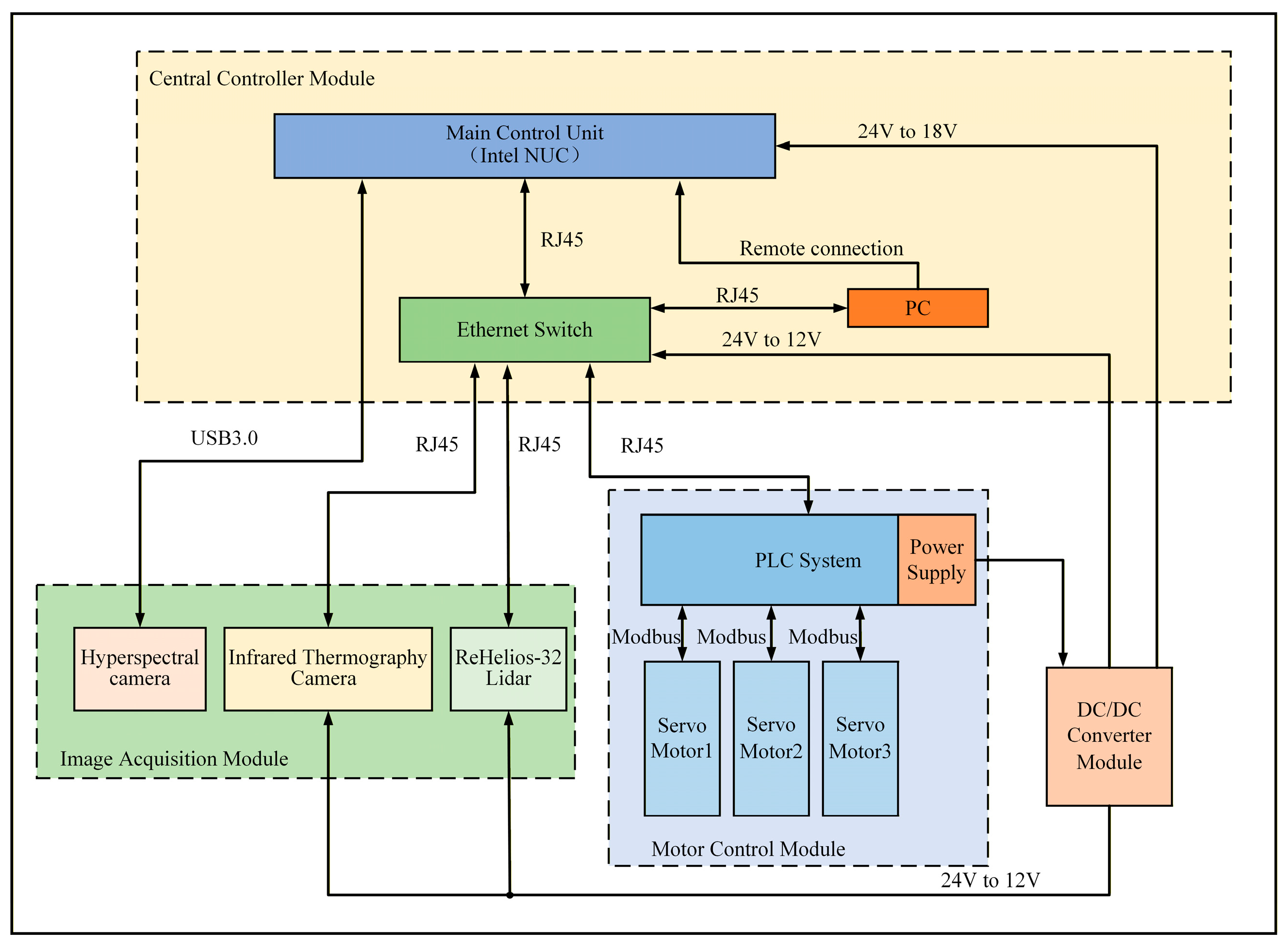
Part C contains the Intel NUC10FNH industrial-grade computer (Intel Corporation, Santa Clara, CA, USA), which serves as the phenotyping platform’s central control unit. This unit orchestrates the platform’s motion control, manages sensor operations, and executes real-time data acquisition and processing. A schematic of the control system architecture is shown in
Figure 4.
- (3)
Part D of the platform is the sensor cabin, which combines multiple sensing systems for comprehensive data collection. It is mounted on the truss’s Z-axis and can move vertically to capture images at various plant heights. The cabin contains three sensors. First, an AT61P thermal infrared camera (IRay Technology Co., Ltd., Yantai, China) operates at 12 V, detects temperatures from −20 °C to 150 °C, and provides images at 640 × 512 pixels with ±2 °C accuracy; it is used to monitor plant water status. Second, an FS-22 hyperspectral camera (Hangzhou CHNSpec Technology Co., Ltd., Hangzhou, China) runs on an internal 18 V battery, offers 640 × 480 pixel resolution, automatic focusing, and a spectral range of 400–1000 nm, enabling assessment of plant physiological and biochemical characteristics. Third, an RSHelios LiDAR unit (RoboSense Technology Co., Ltd., Shenzhen, China). It installed in a fixed position within the sensor cabin, mounted on the truss’s Z-axis. The LiDAR performs mechanical spinning (rotating) scans with 32 channels, covering a full 360° horizontally and 26° vertically, with a horizontal angular resolution of 0.4°. The sensor acquires point clouds at a frequency of 20 Hz and stores the data in PCD format. This configuration enables high-density 3D capture of plant structures across multiple heights during platform movement.
All sensors are networked to the industrial computer via Ethernet or USB 3.0 interfaces. Their initialization, synchronization, and acquisition operations are centrally controlled by custom software developed in-house to ensure timing consistency among all sensing modules.
2.3. Data Acquisition System
A centralized data acquisition and control system was developed to synchronize the multi-sensor payload and the gantry motion. The core software, built using C# on the Visual Studio 2022 platform, integrates the Software Development Kits (SDKs) from each sensor manufacturer and operates on the industrial control computer (IPC). This system provides unified scheduling and coordinated control over the hyperspectral camera, thermal infrared imager, LiDAR scanner, and the three-axis gantry, ensuring stable operation and data integrity.
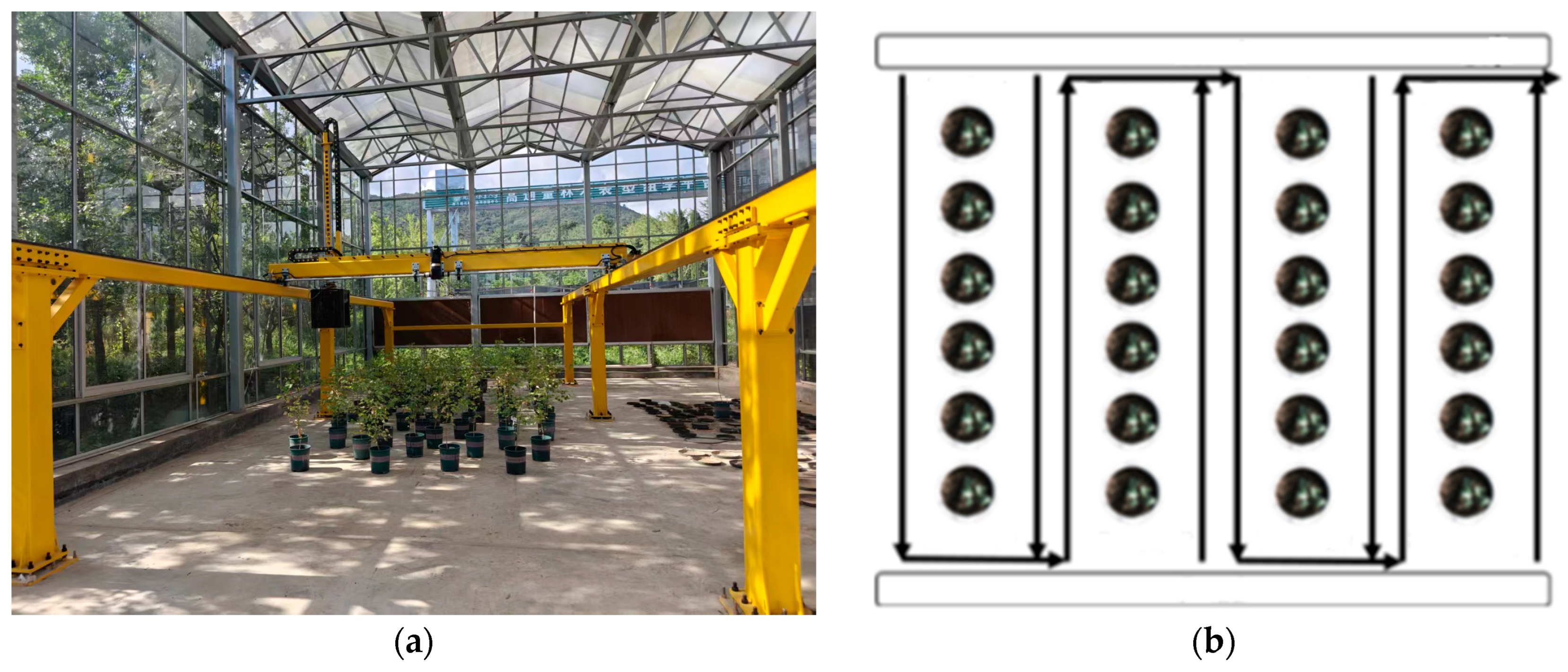
The platform supports two distinct acquisition modes tailored for different experimental needs (
Figure 5):
In fixed-point mode, the sensor unit hovers above a selected plant, and data capture is initiated manually through the software. This approach maintains precise spatial alignment among the hyperspectral, thermal, and LiDAR images, ensuring reliable pixel-level fusion. In automated mode, the acquisition path is generated from predefined plant positions. The system triggers sensors automatically during gantry movement, allowing fast, unattended scanning of multiple plants for high-throughput experiments.
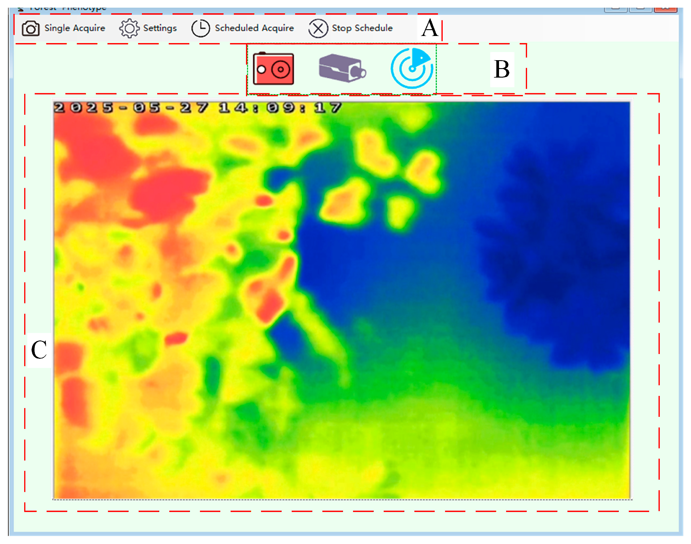
The operation interface of the system appears in
Figure 6. The interface is organized into three main functional modules: (A) the task configuration area, where users can define data acquisition parameters and experiment schedules; (B) the sensor control area, which allows real-time operation of the platform and connected sensors; and (C) the data display area, where acquired data are visualized. Through repeated tests, the gantry movement speed was set to 2 cm s
−1, which provided the best trade-off between data precision and platform stability. When the speed exceeded this value, minor mechanical vibrations appeared, reducing the quality of both hyperspectral images and LiDAR point clouds. Conversely, operating at slower speeds produced redundant data and unnecessarily increased storage requirements.
2.4. Data Processing Framework
Raw data from the platform’s multiple sensors included substantial background interference from soil surfaces, pot edges, and imaging artifacts. To address these issues, we developed a preprocessing pipeline in Python 3.8 with OpenCV and the Point Cloud Library (PCL). Each sensor type required custom processing workflows to eliminate noise and isolate canopy regions. The resulting aligned datasets provided a solid foundation for extracting phenotypic features relevant to water stress analysis.
2.4.1. Thermal Infrared Data Processing for Canopy Temperature Extraction
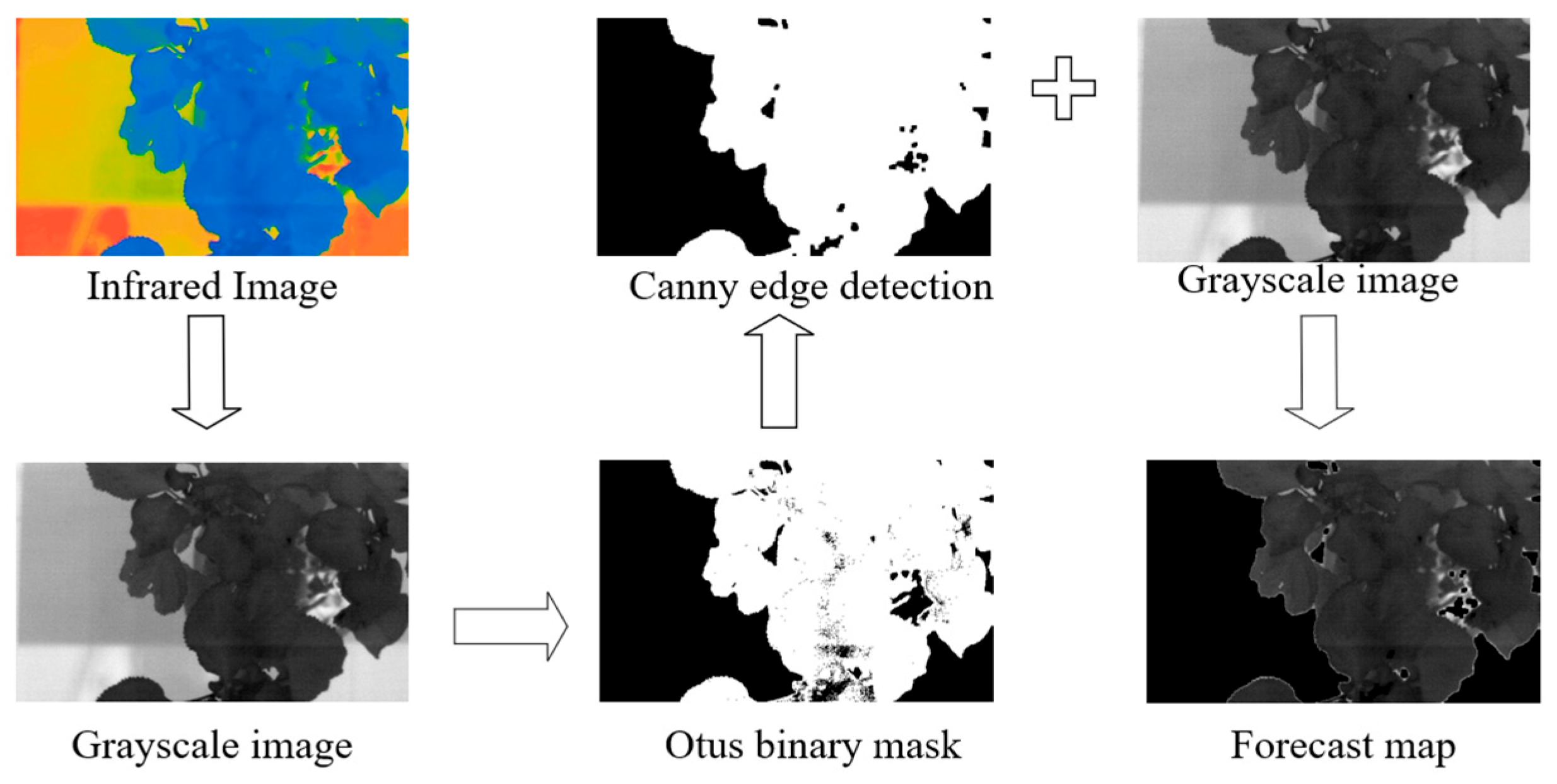
Thermal infrared image directly measures canopy temperature, which reflects plant water status. However, accurate temperature retrieval requires effective separation of the canopy from the background. A hybrid segmentation algorithm combining Otsu thresholding and Canny edge detection was used [
31]. Otsu’s method provided an initial segmentation based on pixel intensity, while Canny edge detection refined canopy boundaries and removed isolated noise. The resulting mask preserved the canopy structure well, ensuring accurate extraction of temperature features (
Figure 7).
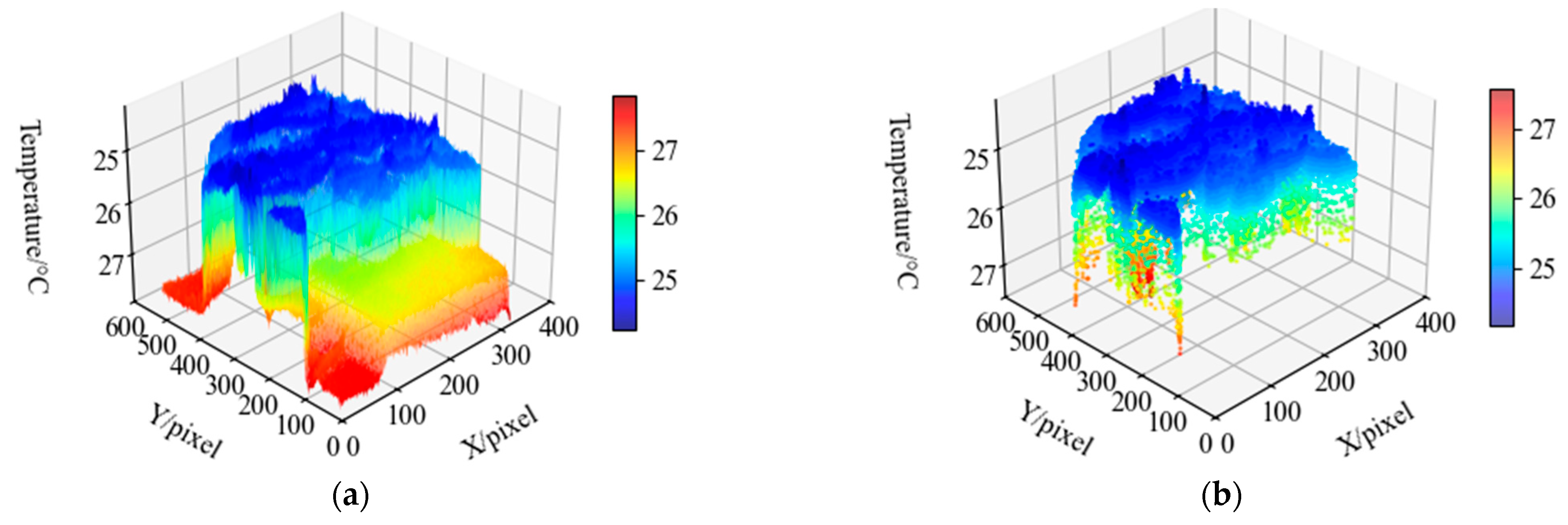
Figure 7 presents 3D thermal maps of the infrared images before and after processing. The raw thermal image (
Figure 8a) exhibited a temperature range influenced by background interference. After segmentation (
Figure 8b), the mask isolated the canopy, leading to a more accurate representation of the plant’s thermal characteristics. The maximum and average temperatures decreased to 27.5 °C and 24.9 °C, respectively, as high-temperature background pixels were removed, while the structural thermal signature of the canopy was preserved.
2.4.2. Hyperspectral Data Processing and Feature Band Selection
Hyperspectral imagery requires careful preprocessing to suppress noise and extract physiologically meaningful information [
32]. The proposed pipeline included three key stages: radiometric calibration, spectral denoising, and feature band selection.
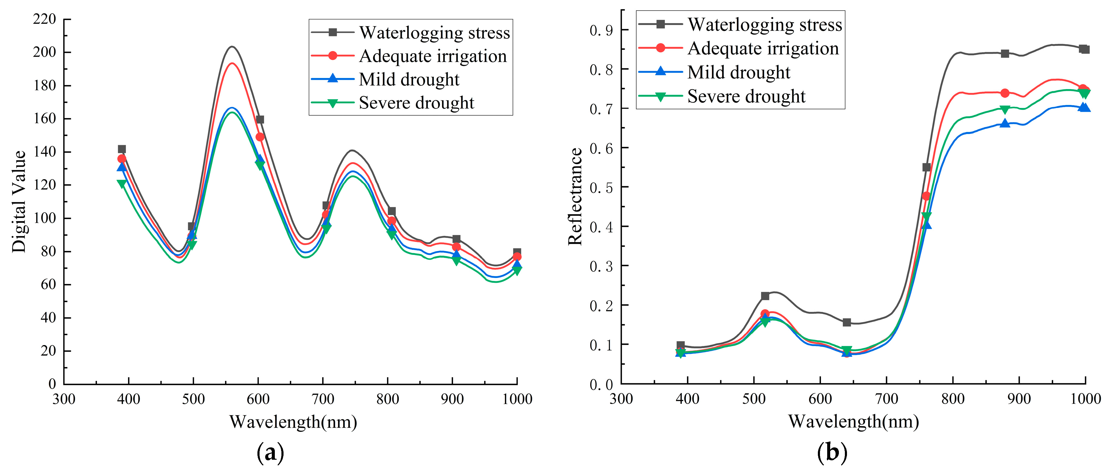
First, raw digital numbers were converted to reflectance values using standard black–white reference calibration, correcting for dark current and illumination non-uniformity. The black and white correction formula is as follows:
R represents the corrected spectral reflectance, I
raw represents the original pixel spectral value, I
black represents the blackboard reflectance spectrum, and I
white represents the whiteboard reflectance. The calibrated spectra were then smoothed with a Savitzky–Golay (SG) filter [
33] to enhance the signal-to-noise ratio while retaining spectral detail (
Figure 9). The spectral curves of plant canopies under different degrees of water stress before and after treatment are shown in
Figure 8.
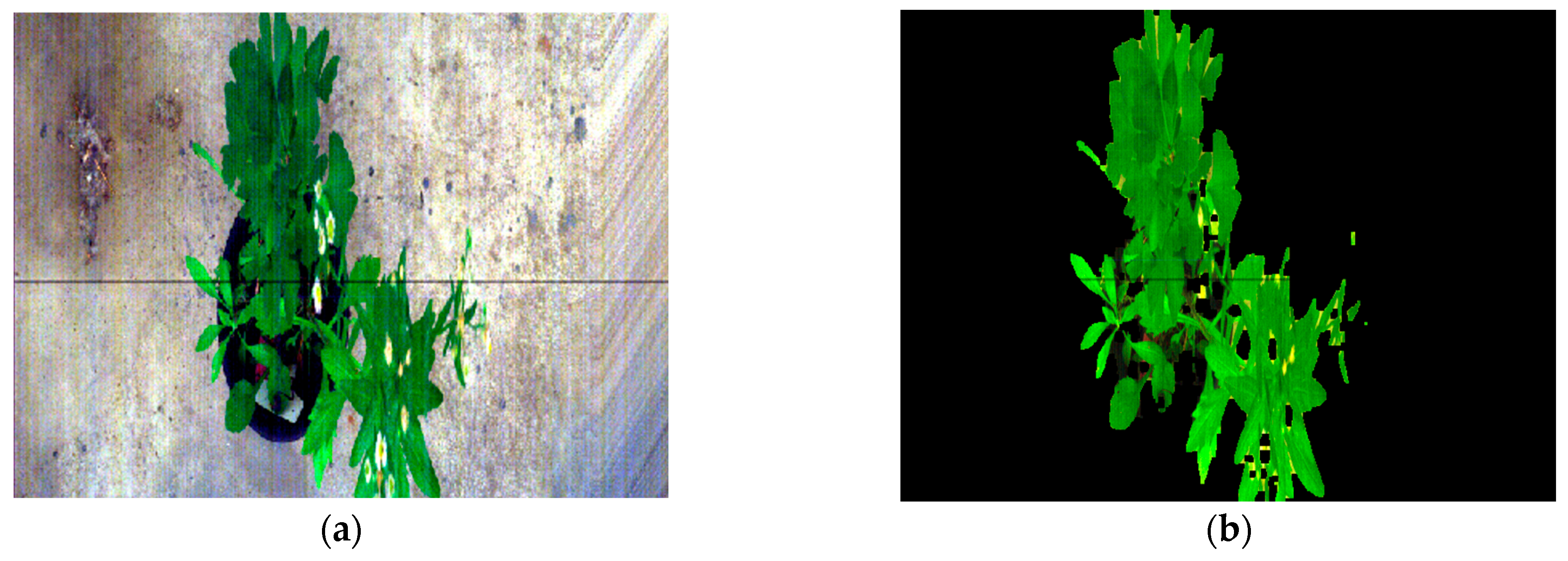
Next, canopy spectra were automatically extracted based on vegetation indices. Specifically, a Normalized Difference Vegetation Index (NDVI) image was generated, and the Otsu algorithm was applied to this image to create a binary mask [
32], effectively separating vegetation (NDVI > 0.4) from the background without manual intervention (
Figure 10). The formula for NDVI calculation is presented as follows:
Finally, to address the high dimensionality of hyperspectral data, we evaluated two feature selection algorithms: the Successive Projections Algorithm (SPA) [
33] and Competitive Adaptive Reweighted Sampling (CARS) [
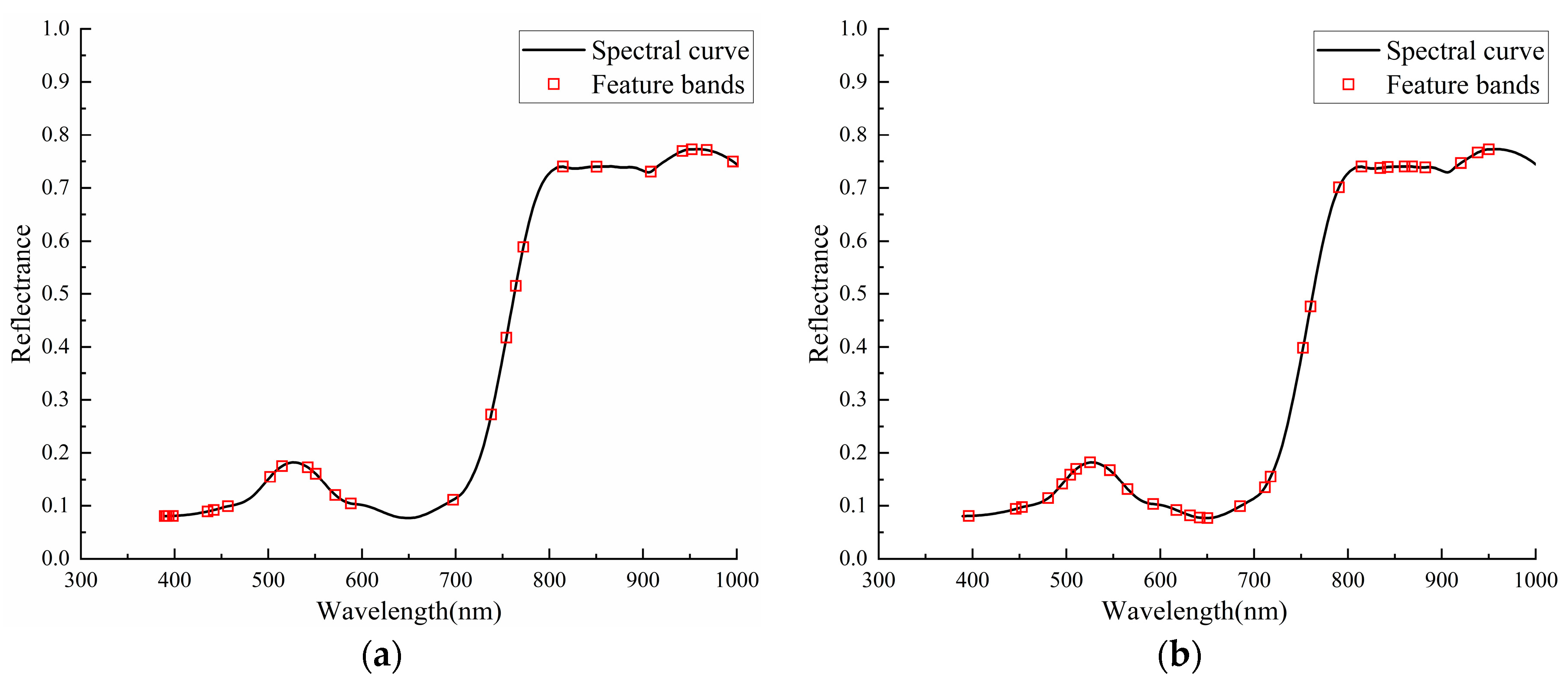
34]. These methods were used to identify the most informative bands related to water stress. As shown in
Figure 11, CARS selected 30 wavelengths that more comprehensively captured key spectral characteristics across the range, including regions associated with chlorophyll absorption (520–580 nm, 640–690 nm) and water content (720–800 nm), and was therefore used for subsequent modeling.
2.4.3. LiDAR Point Cloud Processing for 3D Structure Analysis
The LiDAR point cloud data is stored in PCD format, containing the fields x, y, z, and intensity, which encode the 3D position and return intensity of each point, respectively. The LiDAR point cloud data is stored in PCD format. The result of single-frame sampling is shown in
Figure 11a. Its density is low and it is difficult to reflect the three-dimensional structure of the plant. Therefore, we employed a strategy of multi-frame registration and fusion using the Iterative Closest Point (ICP) algorithm [
35]. By acquiring a sequence of point cloud frames during gantry movement and aligning them based on calculated relative poses, a dense, composite 3D point cloud of the plant was reconstructed (
Figure 12b).
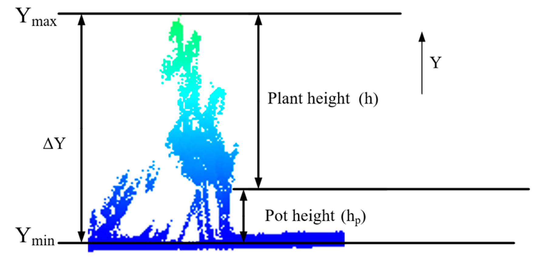
The reconstructed point cloud was then segmented using the DBSCAN clustering algorithm to separate the plant canopy from the ground and pot points. Plant height was calculated as follows: Plant height was calculated as the vertical distance between the highest canopy point (Y
max) and the average height of the ground points (Y
min), with an adjustment for pot height (h
p) (
Figure 13). This method provides an accurate, non-destructive metric of plant growth and structure.
Plant height variation is an important morphological response to water stress. Smith’s study proofed that plant height is closely associated with water availability and stress levels [
36]. In this study, LiDAR-derived plant height was not incorporated into the multi-modal fusion model. Instead, it was used as an independent indicator to assist in the analysis and to validate the performance of the proposed water stress detection models. Plant height measured using LiDAR can help evaluate the growth differences under different water stress treatments. They supplied another structural data to explain what we learned from hyperspectral and thermal imaging. This combined approach makes the assessment easier to interpret.
2.5. Development of a Multi-Sensor Fusion Model for Water Stress Detection
To achieve reliable identification of plant water stress levels, we constructed a machine learning model that combines hyperspectral and thermal infrared features. The model employs a Kernel Extreme Learning Machine (KELM) to capture the nonlinear patterns in the data. To further improve the representation of multi-source information, the method was extended to a Multi-Kernel ELM (MK-ELM), whose hyperparameters were optimized using the Whale Optimization Algorithm (WOA).
2.5.1. Kernel Extreme Learning Machine (KELM)
The Extreme Learning Machine (ELM) is known for its computational efficiency but can be unstable due to the random initialization of its hidden layer [
37]. The KELM incorporates a kernel function, which implicitly maps the input features into a high-dimensional space, thereby enhancing stability and generalization performance. In this study, the Gaussian (RBF) kernel is applied (Formula (4)). The Gaussian kernel function has good generalization performance in processing nonlinear distribution features such as plant hyperspectral and thermal infrared [
38,
39].
For a given training sample,
where N is the number of samples,
d is the feature dimension, and
m is the output dimension. The kernel matrix is constructed as Formula (5).
Although KELM performs well for small, high-dimensional datasets, it processes multi-source heterogeneous data uniformly. It ignores the differences in distribution characteristics, scale sensitivity, and semantic expression among different types of features [
40]. Therefore, an improved method is needed to account for the structural variations between different feature subspaces and improve model accuracy.
2.5.2. Whale Optimization Algorithm-Based Multi-Kernel ELM (WOA-MK-ELM)
To address the challenge, we extended KELM to Multi-Kernel Extreme Learning Machine (MK-ELM). Specifically, separate Gaussian kernel functions are defined for the hyperspectral feature subspace (K
HSI), and the thermal infrared feature subspace (K
TIR). The fused kernel matrix is obtained by a weighted combination:
where μ ∈ [0, 1] is the kernel combination weight coefficient, which is used to control the contribution of the two kernel functions to the final kernel space. The training process of MK-ELM is similar to KELM model, and its output is as follows:
While this multi-kernel design allows the model to better exploit complementary information between hyperspectral and thermal features, it also introduces additional hyperparameters, including the two kernel function width parameters σ1 and σ2, the fusion weight coefficient μ, and the regularization parameter C.
To eliminate the need for manual parameter tuning during model training, the Whale Optimization Algorithm (WOA) [
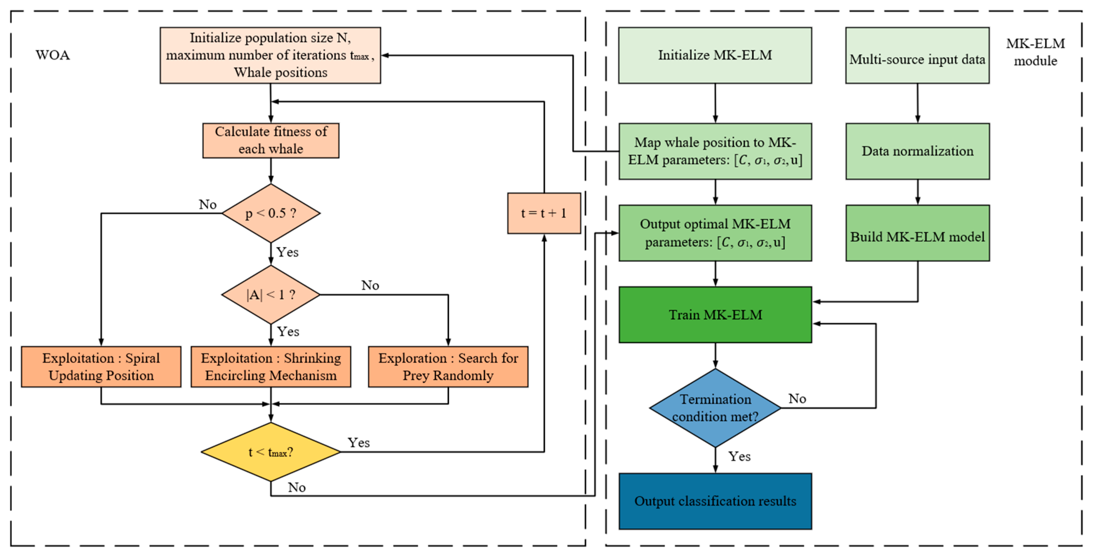
41] was employed to optimize the MK-ELM framework, resulting in the WOA-MK-ELM variant. This approach automatically identifies the optimal hyperparameters. The corresponding training workflow is depicted in
Figure 14.
In the WOA-MK-ELM framework, each whale represents a potential hyperparameter set (C, σ1, σ2, μ). In this setup, each whale represents a possible solution, and we assess its quality based on the model’s classification accuracy. The optimization process seeks a high-accuracy solution by strategically exploiting promising regions while also exploring the search space broadly to avoid local optima. Once the algorithm converges, we retrain the MK-ELM model with the optimized hyperparameters to produce the final classifier.
2.6. Evaluation Metrics
To evaluate the performance of each model, accuracy, precision, recall, and F1-score were used as evaluation indicators, and confusion matrix was used for visualization. In theory, it is expected that both precision and recall will remain high, but you cannot have both. To comprehensively measure these two metrics and find a balance, the F1-score is introduced as a harmonic mean. The F1-score aims to simultaneously take into account high precision and recall. Its value range is [0, 1], with an optimal value of 1. The calculation formulas for each metric are as follows:
3. Results
3.1. Feature Extraction and Single-Source Model Performance
First, we constructed a single-source classification model based on hyperspectral images. The hyperspectral image processing method proposed in
Section 2.4.2 was used for hyperspectral data.
Figure 15 is a pseudo-color image of the
Perilla canopy after processing the hyperspectral raw image data. From left to right are the T1–T4 treatment groups, corresponding to levels I–IV of water stress. The characteristic wavelength selection results are shown in
Table 1.
Subsequently, a KELM water stress degree detection model based on different characteristic wavelengths is constructed. The reflectance of different characteristic bands is used as the input of the model, and the output is the water stress level to evaluate the performance of different band combinations in the detection model.
A significant correlation exists between plant canopy temperature characteristics and key physiological parameters, namely leaf stomatal conductance and transpiration rate [
42]. Consequently, canopy temperature serves as an indirect indicator of leaf water utilization, enabling the diagnosis of plant water stress status.
Figure 16 presents the spatial distribution of canopy temperature under varying stress conditions. Within this thermal map, the color gradient corresponds to temperature values: black denotes the minimum temperature in the range, while increasing color intensity signifies progressively higher temperatures.
Observing
Figure 16, as water stress intensifies, the canopy temperature of plants increases, which is consistent with the conclusion of the plant canopy temperature and plant water stress response mentioned in the literature [
43]. For the treated plant canopy foreground image, the temperature characteristics are calculated, including the maximum temperature, minimum temperature, average temperature, and temperature variance value to construct a thermal characteristic matrix. The first three quantities reflect the plant canopy temperature characteristic quantity itself, and the last one reflects the degree of temperature dispersion.
3.2. Multi-Source Data Fusion for Enhanced Diagnosis
Information fusion, also known as multi-sensor information fusion (MSIF), uses different sensors to sample the target object. It then analyzes, correlates, and optimizes the multi-source data according to predefined criteria to support decision-making tasks. Information fusion is mainly divided into three levels: input-level fusion, feature-level fusion, and decision-level fusion [
44]. In order to give full play to the complementary advantages of multi-source data, this study proposes a fusion model that integrates hyperspectral and thermal infrared information, and evaluates it from two perspectives: input-level fusion and feature-level fusion.
Input layer fusion is used to directly splice the hyperspectral features and temperature features to form a unified feature vector as the model input. This method maintains the integrity of the original features and facilitates the direct integration of multi-source information. KELM is used to model and evaluate the water stress classification performance of multi-source feature fusion.
In order to further improve the flexibility and expressiveness of the fusion model, this paper adopts a feature layer fusion strategy based on multi-kernel learning (MKL) [
45]. This method selects different Gaussian kernel functions to map multi-source data, and on this basis, constructs the MK-ELM model to achieve feature fusion through weighted kernel combination. In the model, the kernel function weights and KELM parameters are optimized by the WOA. This method not only retains the independent structural characteristics of each modal data, but also explores their complementarity, thus improving the model’s discriminative ability. The modeling idea is shown in
Figure 17.
3.3. Test Results
This section details the partitioning of the collected dataset into training and test subsets using a 7:3 ratio for model development and performance assessment. The evaluation commenced with single-source data models to quantify their classification accuracy. Subsequently, the optimal single-source approach was selected to construct a multi-source data fusion framework. A comparative assessment of all models was then conducted to evaluate the efficacy of distinct data sources and fusion methodologies.
The results are shown in
Table 2, demonstrating the accuracy of the characteristic wavelength model. It can be seen that the accuracy of the test set and the training set under each model is similar, among which the CARS-KELM model has the highest accuracy, followed by the full-band, and the SPA + KELM model has the lowest accuracy. Therefore, the CARS algorithm was used to extract the characteristic bands as the input of the fusion model.
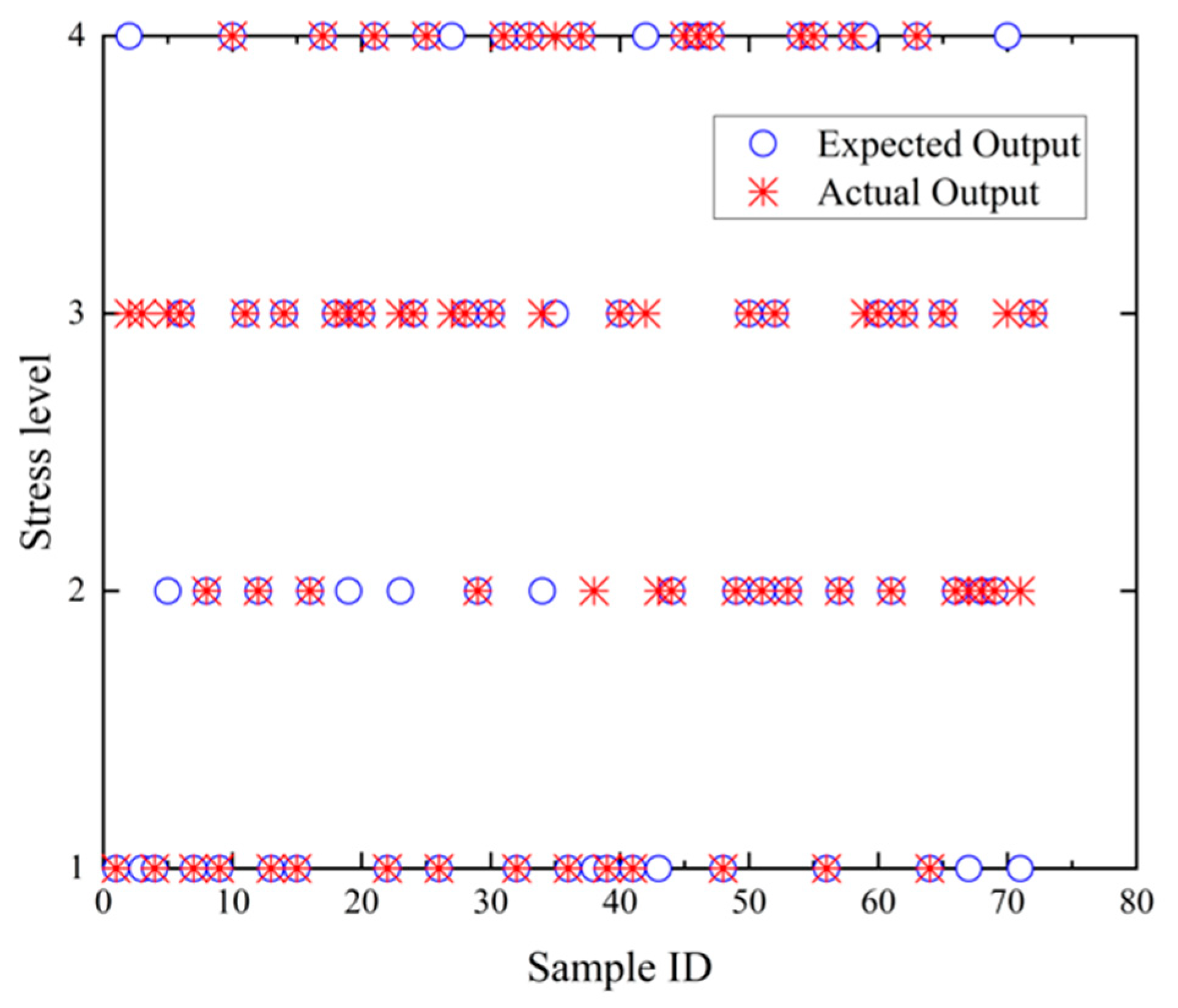
We calculate and extract temperature features based on thermal infrared images, and train the KELM model. The accuracy of the model on the test set reaches 81.17%. Cross-validation results further verified the model’s stability, with an average accuracy of 78.51%.
Figure 18 presents an example subset of the model outputs based on thermal infrared temperature features. In this representative subset, the temperature-based model correctly identified 57 samples and incorrectly identified 15. Misclassifications included five samples labeled as Level I, four as Level II, one as Level III, and five as Level IV water stress. These results illustrate the inherent difficulty of accurately determining plant water stress levels using temperature features alone, as the feature space exhibits noticeable overlap across classes.
Using the idea shown in
Figure 17, we constructed the MK-ELM model. This study used two data sources. After feature extraction, we generated two feature spaces, A and B. These spaces were mapped to two similar spaces using a Gaussian kernel function. These spaces were then used to construct a combined space, and the WOA was used for automatic hyperparameter optimization. Ultimately, the WOA-MK-ELM water stress detection model was established.
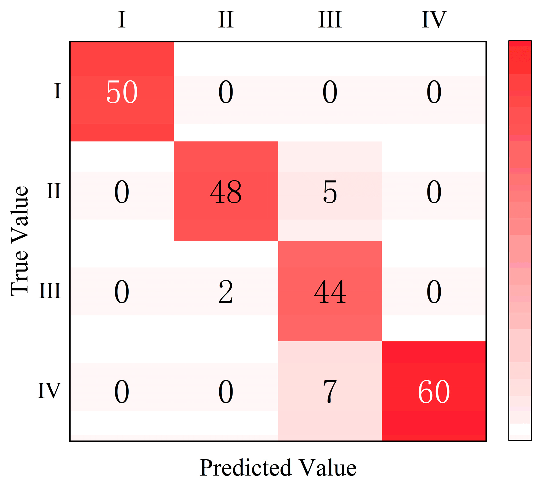
Figure 19 shows the confusion matrix of the model based on feature layer fusion. The overall prediction accuracy of this model was 93.52%, exceeding that of the input layer fusion model.
Table 3 lists the model evaluation metrics calculated based on this confusion matrix.
The feature-layer fusion model not only achieved an overall prediction accuracy of 93.52% but also achieved an F1-Score exceeding 0.86 for all levels of samples, demonstrating excellent prediction results for all types of samples. With average precision and recall rates around 93%, and an average F1-Score of 0.93, the model outperformed detection models based on input-layer fusion.
To further validate the model’s predictions, we examined structural information derived from LiDAR point clouds. Although plant height was not used as an input feature in the multi-modal fusion model, it served as an independent metric for supporting model validation. We used Pearson correlation analysis to examine the relationship between LiDAR-derived plant height and predicted water stress levels. The results revealed a moderately strong negative correlation (r = −0.70, p < 0.05), meaning that plants subjected to higher water stress exhibited reduced height. This finding supported that plant height decreases under water deficit. It provides additional evidence that the models accurately capture plant responses to water deficit.
3.4. Comparison of Different Models
This section compares the performances of water stress detection models based on different data modalities and fusion strategies. In addition, we used different machine learning models (SVM, RF, and KNN) for a more comprehensive evaluation. All models were trained and tested on the expanded dataset, consisting of 672 multi-sensor samples. The classification accuracy of each model is summarized in
Table 4 and illustrated in
Figure 20.
As is shown in
Table 4, models based on single-source data exhibit moderate classification performance. For KELM models using hyperspectral data, the test set accuracies were 83.73% (all bands), 85.43% (CARS-selected bands), and 80.58% (SPA-selected bands). It indicated that the CARS method effectively captures the most informative wavelengths related to water stress. The KELM model based on thermal infrared features achieved a test accuracy of 81.17%, confirming that thermal characteristics alone can reflect differences in plant water status. However, when used individually, these single-source data are not sufficient to fully distinguish among water stress levels.
By comparison, models utilizing multi-source data achieved clear improvements. The KELM-based input-level fusion model achieved a test accuracy of 89.81%, illustrating the advantage of combining hyperspectral and thermal information. Notably, our proposed WOA-MK-ELM model with feature-level fusion further improved performance, achieving 93.52% test accuracy. These results suggested that feature-level fusion more effectively integrates the information from heterogeneous data sources, yielding higher predictive accuracy and robustness.
In comparison, traditional machine learning models trained on the same multimodal dataset achieved the following results: SVM, 91.2%; RF, 90.5%; KNN, 89.8%. While these models demonstrate reasonable performance, our proposed WOA-MK-ELM model (feature-level fusion) consistently achieved the highest accuracy of 93.06%, along with superior precision, recall, and F1-score across all stress levels. This demonstrates not only the overall effectiveness of the proposed KELM-based multimodal fusion approach but also its robustness and stability relative to conventional algorithms.
In addition, we also used other evaluation metrics, such as precision, recall, and F1-score, to assess model performance. The confusion matrix and performance metric tables for the two fusion models are provided above.
Figure 21 displayed the evaluation metrics of the two different fusion models.
4. Discussion
This research presents a multi-sensor system aimed at addressing ongoing challenges in high-resolution forest health assessment. This research presents a multi-sensor system aimed at addressing ongoing challenges in high-resolution forest health assessment. Comparable phenotyping systems, such as the LemnaTec Scanalyze, Crop3D, and mobile platforms like PhenoRover, have been widely applied to agricultural crops. Our prototype applied these concepts for forestry phenotyping by acquiring thermal, hyperspectral, and LiDAR data synchronously. Its flexible Z-axis mounting and robust multi-sensor calibration allowed for reliable feature-level fusion, even in structurally complex seedlings.
We found that multi-sensor fusion was genuinely useful for plant water stress detection. The WOA-MK-ELM model, combining thermal, spectral, and structural data, gave more consistent and accurate results across stress levels. This improvement mainly comes from the fact that the signal responds at different times during drought progression, which mitigates reliance on any single, potentially variable indicator. Recent studies show a similar trend. Okyere used optimized vegetation indices derived from hyperspectral reflectance and achieved classification accuracies exceeding 0.94 across DNN models under controlled greenhouse conditions [
46]. Gupta developed an RGB-based drought detection framework for wheat, reporting an accuracy of approximately 91.2% using a Random Forest classifier [
47]. In comparison, our WOA-MK-ELM model reached 93.5% classification accuracy under small-sample conditions, demonstrating that it can reliably detect water stress even when limited data are available.
This work also demonstrates how the indoor multi-sensor acquirement system can accelerate methodological progress in forestry monitoring. Using Perilla frutescens as a representative species subjected to graded water stress, we were able to clearly separate the spectral signatures of stress from field variability. This controlled setting enabled stepwise development and testing of a multimodal analysis pipeline. We used segmentation method for accurate thermal and spectral feature extraction to a WOA-optimized multi-kernel fusion model. This workflow is not just a fixed procedure; it can be reused in other settings. It fits both small nursery trials and UAV tree surveys, making it easier to translate indoor findings to real forestry work. To further benchmark our approach, we compared WOA-MK-ELM with common machine learning models trained on the same multi-source dataset. Support Vector Machine (SVM) scored 89.35% test accuracy, Random Forest (RF) reached 84.72%, and K-Nearest Neighbors (KNN) dropped to 76.85%. RF trained well (95.24%), but, its lower test performance indicates potential overfitting. KNN still performed poorly. The fused features were too high-dimensional for it to handle well. Overall, WOA-MK-ELM did better than the other models, and its results were more consistent.
Although this experiment was conducted in a greenhouse, earlier studies confirmed that stress indicators calibrated indoors still work well when applied in more variable field settings. Fiorani and Schurr positioned greenhouse phenotyping as a robust basis for transferring water-stress assessments to field crops [
48]. Sankaran demonstrated that spectral and thermal indicators calibrated in greenhouse trials still hold up when used in field conditions [
49]. This implies that once the physiological meaning of the indicators is established indoors, the same multimodal features can be used in nursery or forest settings with proper calibration. This also means the workflow has practical value outside controlled environments.
Based on these findings, our next step is to test the multimodal sensing workflow outside controlled conditions. We will start with woody seedlings in greenhouse or semi-natural settings, then move on to small field trials in forest plots. These environments feature factors absent indoors, such as heterogeneous soil moisture, variable irradiance, and microclimate fluctuations, which are key to evaluating the robustness of sensor-based drought indicators. If the workflow performs well under these conditions, it would show that the multimodal framework can be used in real forestry monitoring and drought early-warning work.
The framework proved effective in the controlled settings. It still faced several challenges in field applications. First, the use of multiple sensors made the platform more complicated. To adapt the system for field use, simpler hardware or an integrated sensor module would be needed. While the fusion approach worked well indoors, we can add other sensors to improve the ability of early stress detection. LiDAR data could help quantify structural and biomass traits, which will assist widely ecological studies. Finally, the present workflow depends on offline processing, which limits its use for rapid diagnosis. Addressing these points will make the framework suitable for practical forestry applications.
5. Conclusions
In response to the escalating impacts of climate change on global forest ecosystems, this study built a prototype system combining multiple sensors to monitor plant water status in a greenhouse. This work provides an initial step toward integrating hyperspectral, thermal infrared, and LiDAR sensing for vegetation stress assessment.
The principal contributions of this work are threefold: (1) We engineered an integrated hardware-software platform capable of synchronizing hyperspectral, thermal infrared, and LiDAR sensors. It enabled co-captured multimodal datasets which suitable for forests monitor algorithm development and testing. (2) We established a comprehensive data processing pipeline that extracts and integrates physiological, functional, and structural features from heterogeneous sources. (3) The resulting WOA-MK-ELM model, implementing adaptive multi-kernel learning, achieved 93.56% accuracy in plant water stress classification, confirming the superiority of feature-level fusion over single-source or input-level alternatives.
In summary, this study offers a promising proof-of-concept for multimodal sensing–based plant stress detection and provides a foundation for future extensions. Nevertheless, the findings remain constrained by the controlled environment, limited sample size, and single-species design. Future work will expand the system to nursery and forest conditions, incorporate more diverse plant materials, and further evaluate the generalization and robustness of the proposed framework.
Author Contributions
Conceptualization, Y.W., Q.F. and J.Z.; methodology, Y.W., Q.F. and J.Z.; software, J.Z.; validation, Y.W., S.Q. and J.Z.; formal analysis, Y.L. and Y.W.; investigation, J.Z. and S.Q.; resources, Y.W. and Y.L.; data curation, J.Z. and S.Q.; writing—original draft preparation, J.Z.; writing—review and editing, Y.W., S.Q., Y.L. and J.Z.; visualization, Y.W. and J.Z.; supervision, Y.W. and Y.L.; project administration, Y.W. and Y.L.; funding acquisition, Y.W., Q.F. and Y.L. All authors have read and agreed to the published version of the manuscript.
Funding
This work was supported in part by the Biological Breeding-National Science and Technology Major Project under grant 2023ZD0405605, by the Sichuan Yibin Bamboo Industry Major Public Project under grant YBZD2024, by the National Natural Science Foundation of China under grant 32171788 and, in part, by the Qing Lan Project of Jiangsu colleges and universities.
Data Availability Statement
All data generated or presented in this study are available upon request from corresponding author. Furthermore, the models and code used during this study cannot be shared at this time as the data also form part of an ongoing study.
Acknowledgments
The authors would like to thank the editor and the anonymous reviewers for their valuable suggestions for improving the quality of this paper.
Conflicts of Interest
The authors declare no conflicts of interest.
References
- Yang, G.; Chang, J.; Wang, Y.; Guo, A.; Zhang, L.; Zhou, K.; Wang, Z. Understanding drought propagation through coupling spatiotemporal features using vine copulas: A compound drought perspective. Sci. Total Environ. 2024, 921, 171080. [Google Scholar] [CrossRef]
- Zhang, G.; Huimin, W.; Xiaoling, S.; Hongyuan, F.; Zhang, S.; Huang, J.; Kai, F. Assessing the vegetation vulnerability of Loess Plateau under compound dry and hot climates. Trans. Chin. Soc. Agric. Eng. 2024, 40, 339–346. [Google Scholar]
- Bian, L.-M.; Zhang, H.-C. Application of phenotyping techniques in forest tree breeding and precision forestry. CABI Datebases 2020, 56, 113–126. [Google Scholar]
- Zhao, C.-J. Big data of plant phenomics and its research progress. CABI Datebases 2019, 1, 5–18. [Google Scholar]
- He, Y.; Li, X.; Yang, G. Research progress and prospect of indoor high-throughput germplasm phenotyping platforms. Trans. CSAE 2022, 38, 127–141. [Google Scholar]
- Pieruschka, R.; Schurr, U. Plant phenotyping: Past, present, and future. Plant Phenomics 2019, 2019, 7507131. [Google Scholar] [CrossRef] [PubMed]
- Wang, J.; Ding, C.; Li, W.; Luo, K.; Wang, J.; Zhang, W.; Niu, S.; Zhang, M.; Zhao, X.; Xue, L.; et al. Progress in Genetic Breeding of Forest Trees in China, 2024. For. Sci. 2025, 61, 35–51. [Google Scholar] [CrossRef]
- Cohen, Y.; Alchanatis, V.; Prigojin, A.; Levi, A.; Soroker, V.; Cohen, Y. Use of aerial thermal imaging to estimate water status of palm trees. Precis. Agric. 2012, 13, 123–140. [Google Scholar] [CrossRef]
- Saarinen, N.; Vastaranta, M.; Näsi, R.; Rosnell, T.; Hakala, T.; Honkavaara, E.; Wulder, M.A.; Luoma, V.; Tommaselli, A.; Imai, N. UAV-based photogrammetric point clouds and hyperspectral imaging for mapping biodiversity indicators in boreal forests. Int. Arch. Photogramm. Remote Sens. Spat. Inf. Sci. 2017, 42, 171–175. [Google Scholar] [CrossRef]
- Roitsch, T.; Cabrera-Bosquet, L.; Fournier, A.; Ghamkhar, K.; Jiménez-Berni, J.; Pinto, F.; Ober, E.S. New sensors and data-driven approaches—A path to next generation phenomics. Plant Sci. 2019, 282, 2–10. [Google Scholar] [CrossRef]
- Singh, A.; Jones, S.; Ganapathysubramanian, B.; Sarkar, S.; Mueller, D.; Sandhu, K.; Nagasubramanian, K. Challenges and opportunities in machine-augmented plant stress phenotyping. Trends Plant Sci. 2021, 26, 53–69. [Google Scholar] [CrossRef]
- Su, B.; Liu, Y.; Huang, Y.; Wei, R.; Cao, X.; Han, D. Analysis for stripe rust dynamics in wheat population using UAV remote sensing. Trans. CSAE 2021, 37, 127–135. [Google Scholar]
- Yang, W.; Feng, H.; Zhang, X.; Zhang, J.; Doonan, J.H.; Batchelor, W.D.; Xiong, L.; Yan, J. Crop phenomics and high-throughput phenotyping: Past decades, current challenges, and future perspectives. Mol. Plant 2020, 13, 187–214. [Google Scholar] [CrossRef]
- Hu, W.; Fu, X.; Chen, F.; Yang, W. A path to next generation of plant phenomics. Chin. Bull. Bot. 2019, 54, 558. [Google Scholar]
- Du, J.; Lu, X.; Fan, J.; Qin, Y.; Yang, X.; Guo, X. Image-based high-throughput detection and phenotype evaluation method for multiple lettuce varieties. Front. Plant Sci. 2020, 11, 563386. [Google Scholar] [CrossRef]
- González-Dugo, V.; Testi, L.; Villalobos, F.J.; López-Bernal, A.; Orgaz, F.; Zarco-Tejada, P.J.; Fereres, E. Empirical validation of the relationship between the crop water stress index and relative transpiration in almond trees. Agric. For. Meteorol. 2020, 292, 108128. [Google Scholar] [CrossRef]
- Still, C.J.; Rastogi, B.; Page, G.F.; Griffith, D.M.; Sibley, A.; Schulze, M.; Hawkins, L.; Pau, S.; Detto, M.; Helliker, B.R. Imaging canopy temperature: Shedding (thermal) light on ecosystem processes. New Phytol. 2021, 230, 1746–1753. [Google Scholar] [CrossRef] [PubMed]
- Zhang, N.; Li, P.-C.; Liu, H.; Huang, T.-C.; Liu, H.; Kong, Y.; Dong, Z.-C.; Yuan, Y.-H.; Zhao, L.-L.; Li, J.-H. Water and nitrogen in-situ imaging detection in live corn leaves using near-infrared camera and interference filter. Plant Methods 2021, 17, 117. [Google Scholar] [CrossRef]
- Liu, H.; Bruning, B.; Garnett, T.; Berger, B. Hyperspectral imaging and 3D technologies for plant phenotyping: From satellite to close-range sensing. Comput. Electron. Agric. 2020, 175, 105621. [Google Scholar] [CrossRef]
- Sankaran, S.; Quirós, J.J.; Miklas, P.N. Unmanned aerial system and satellite-based high resolution imagery for high-throughput phenotyping in dry bean. Comput. Electron. Agric. 2019, 165, 104965. [Google Scholar] [CrossRef]
- Zhu, X.; Skidmore, A.K.; Darvishzadeh, R.; Wang, T. Estimation of forest leaf water content through inversion of a radiative transfer model from LiDAR and hyperspectral data. Int. J. Appl. Earth Obs. Geoinf. 2019, 74, 120–129. [Google Scholar] [CrossRef]
- Biswas, A.; Sarkar, S.; Das, S.; Dutta, S.; Choudhury, M.R.; Giri, A.; Bera, B.; Bag, K.; Mukherjee, B.; Banerjee, K. Water scarcity: A global hindrance to sustainable development and agricultural production—A critical review of the impacts and adaptation strategies. Camb. Prism. Water 2025, 3, e4. [Google Scholar] [CrossRef]
- Bartlett, M.K.; Klein, T.; Jansen, S.; Choat, B.; Sack, L. The correlations and sequence of plant stomatal, hydraulic, and wilting responses to drought. Proc. Natl. Acad. Sci. USA 2016, 113, 13098–13103. [Google Scholar] [CrossRef]
- Li, H.; Jia, S.; Tang, Y.; Jiang, Y.; Yang, S.; Zhang, J.; Yan, B.; Wang, Y.; Guo, J.; Zhao, S. A transcriptomic analysis reveals the adaptability of the growth and physiology of immature tassel to long-term soil water deficit in Zea mays L. Plant Physiol. Biochem. 2020, 155, 756–768. [Google Scholar] [CrossRef]
- Munns, R.; Millar, A.H. Seven plant capacities to adapt to abiotic stress. J. Exp. Bot. 2023, 74, 4308–4323. [Google Scholar] [CrossRef]
- Sims, D.A.; Gamon, J.A. Relationships between leaf pigment content and spectral reflectance across a wide range of species, leaf structures and developmental stages. Remote Sens. Environ. 2002, 81, 337–354. [Google Scholar] [CrossRef]
- Marchin, R.M.; Ossola, A.; Leishman, M.R.; Ellsworth, D.S. A simple method for simulating drought effects on plants. Front. Plant Sci. 2020, 10, 1715. [Google Scholar] [CrossRef] [PubMed]
- Virlet, N.; Sabermanesh, K.; Sadeghi-Tehran, P.; Hawkesford, M.J. Field Scanalyzer: An automated robotic field phenotyping platform for detailed crop monitoring. Funct. Plant Biol. 2016, 44, 143–153. [Google Scholar] [CrossRef] [PubMed]
- Guo, Q.; Wu, F.; Pang, S.; Zhao, X.; Chen, L.; Liu, J.; Xue, B.; Xu, G.; Li, L.; Jing, H. Crop 3D—A LiDAR based platform for 3D high-throughput crop phenotyping. Sci. China Life Sci. 2018, 61, 328–339. [Google Scholar] [CrossRef] [PubMed]
- Xu, R.; Li, C. A review of high-throughput field phenotyping systems: Focusing on ground robots. Plant Phenomics 2022, 2022, 9760269. [Google Scholar] [CrossRef]
- Otsu, N. A threshold selection method from gray-level histograms. Automatica 1975, 11, 23–27. [Google Scholar] [CrossRef]
- Long, Y.-W.; Li, M.-Z.; Gao, D.-H.; Zhang, Z.-Y.; Sun, H.; Qin, Z. Chlorophyll content detection based on image segmentation by plant spectroscopy. Spectrosc. Spectr. Anal. 2020, 40, 2253–2258. [Google Scholar]
- Araújo, M.C.U.; Saldanha, T.C.B.; Galvao, R.K.H.; Yoneyama, T.; Chame, H.C.; Visani, V. The successive projections algorithm for variable selection in spectroscopic multicomponent analysis. Chemom. Intell. Lab. Syst. 2001, 57, 65–73. [Google Scholar] [CrossRef]
- Liu, Y.-H.; Wang, Q.-Q.; Shi, X.-W.; Gao, X. Hyperspectral nondestructive detection model of chlorogenic acid content during storage of honeysuckle. Trans. Chin. Soc. Agric. Eng. 2019, 35, 291–299. [Google Scholar]
- Besl, P.J.; McKay, N.D. Method for registration of 3-D shapes. In Proceedings of the Sensor Fusion IV: Control Paradigms and Data Structures, Boston, MA, USA, 12–15 November 1992; pp. 586–606. [Google Scholar]
- Smith, D.D.; Sperry, J.S. Coordination between water transport capacity, biomass growth, metabolic scaling and species stature in co-occurring shrub and tree species. Plant Cell Environ. 2014, 37, 2679–2690. [Google Scholar] [CrossRef] [PubMed]
- Rakesh, S.; Sudhakar, P. Deep transfer learning with optimal kernel extreme learning machine model for plant disease diagnosis and classification. Int. J. Electr. Eng. Technol. IJEET 2020, 11, 160–178. [Google Scholar]
- Chen, C.; Li, W.; Su, H.; Liu, K. Spectral-spatial classification of hyperspectral image based on kernel extreme learning machine. Remote Sens. 2014, 6, 5795–5814. [Google Scholar] [CrossRef]
- Janssens, O.; Van de Walle, R.; Loccufier, M.; Van Hoecke, S. Deep learning for infrared thermal image based machine health monitoring. IEEE/ASME Trans. Mechatron. 2017, 23, 151–159. [Google Scholar] [CrossRef]
- Gu, Y.; Chanussot, J.; Jia, X.; Benediktsson, J.A. Multiple kernel learning for hyperspectral image classification: A review. IEEE Trans. Geosci. Remote Sens. 2017, 55, 6547–6565. [Google Scholar] [CrossRef]
- Mirjalili, S.; Lewis, A. The whale optimization algorithm. Adv. Eng. Softw. 2016, 95, 51–67. [Google Scholar] [CrossRef]
- Zhang, Z.; Bian, J.; Han, W.; Fu, Q.; Chen, S.; Cui, T. Cotton moisture stress diagnosis based on canopy temperature characteristics calculated from UAV thermal infrared image. Nongye Gongcheng Xuebao/Trans. Chin. Soc. Agric. Eng. 2018, 34, 77–84. [Google Scholar]
- Chen, S.; Chen, Y.; Chen, J.; Zhang, Z.; Fu, Q.; Bian, J.; Cui, T.; Ma, Y. Retrieval of cotton plant water content by UAV-based vegetation supply water index (VSWI). Int. J. Remote Sens. 2020, 41, 4389–4407. [Google Scholar] [CrossRef]
- Duan, L.; Li, T.; Tang, Y.; Yang, J.; Liu, W. Mechanical fault diagnosis method based on multi-source heterogeneous information fusion. Pet. Mach. 2021, 49, 60–67. [Google Scholar]
- Schlegel, R.; Chow, C.-Y.; Huang, Q.; Wong, D.S. User-defined privacy grid system for continuous location-based services. IEEE Trans. Mob. Comput. 2015, 14, 2158–2172. [Google Scholar] [CrossRef]
- Okyere, F.G.; Cudjoe, D.K.; Virlet, N.; Castle, M.; Riche, A.B.; Greche, L.; Mohareb, F.; Simms, D.; Mhada, M.; Hawkesford, M.J. Hyperspectral imaging for phenotyping plant drought stress and nitrogen interactions using multivariate modeling and machine learning techniques in wheat. Remote Sens. 2024, 16, 3446. [Google Scholar] [CrossRef]
- Gupta, A.; Kaur, L.; Kaur, G. Drought stress detection technique for wheat crop using machine learning. PeerJ Comput. Sci. 2023, 9, e1268. [Google Scholar] [CrossRef] [PubMed]
- Sankaran, S.; Espinoza, C.Z.; Hinojosa, L.; Ma, X.; Murphy, K. High-Throughput Field Phenotyping to Assess Irrigation Treatment Effects in Quinoa. Agrosystems Geosci. Environ. 2019, 2, 1–7. [Google Scholar] [CrossRef]
- Fiorani, F.; Schurr, U. Future scenarios for plant phenotyping. Annu. Rev. Plant Biol. 2013, 64, 267–291. [Google Scholar] [CrossRef] [PubMed]
Figure 1.
Experimental process and collected data. (A) Experimental site and information collection platform setup. (B) Soil moisture monitoring. (C) Soil moisture monitoring results of different treatment groups. (D) Partial data collection.
Figure 1.
Experimental process and collected data. (A) Experimental site and information collection platform setup. (B) Soil moisture monitoring. (C) Soil moisture monitoring results of different treatment groups. (D) Partial data collection.
Figure 2.
Composition of Multi-sensor Plant Phenotyping System.
Figure 2.
Composition of Multi-sensor Plant Phenotyping System.
Figure 3.
Actual composition of Multi-sensor System. (A) Motion control system. (B) Mechanical framework. (C) Main control unit. (D) Sensor acquisition unit.
Figure 3.
Actual composition of Multi-sensor System. (A) Motion control system. (B) Mechanical framework. (C) Main control unit. (D) Sensor acquisition unit.
Figure 4.
The Control System of the multi-sensor platform.
Figure 4.
The Control System of the multi-sensor platform.
Figure 5.
Operation and path planning of the acquisition system: (a) actual operation status; (b) path planning in automatic mode.
Figure 5.
Operation and path planning of the acquisition system: (a) actual operation status; (b) path planning in automatic mode.
Figure 6.
An interface view of the acquisition control software. (A) Task configuration area. (B) Sensor control area. (C) Data display area.
Figure 6.
An interface view of the acquisition control software. (A) Task configuration area. (B) Sensor control area. (C) Data display area.
Figure 7.
Thermal infrared image processing flow.
Figure 7.
Thermal infrared image processing flow.
Figure 8.
Three-dimensional thermal maps of infrared images before and after processing: (a) thermal distribution of the original image; (b) thermal distribution of the canopy foreground image.
Figure 8.
Three-dimensional thermal maps of infrared images before and after processing: (a) thermal distribution of the original image; (b) thermal distribution of the canopy foreground image.
Figure 9.
Spectral curves before and after pretreatment: (a) original hyperspectral curves; (b) spectral curves after black and white correction, denoising, and smoothing filtering.
Figure 9.
Spectral curves before and after pretreatment: (a) original hyperspectral curves; (b) spectral curves after black and white correction, denoising, and smoothing filtering.
Figure 10.
Hyperspectral pseudo-color images before and after processing: (a) original hyperspectral pseudo-color image; (b) processed pseudo-color image of the canopy foreground.
Figure 10.
Hyperspectral pseudo-color images before and after processing: (a) original hyperspectral pseudo-color image; (b) processed pseudo-color image of the canopy foreground.
Figure 11.
Spectral Feature Extraction by Various Techniques: (a) feature wavelength selection using the SPA; (b) feature wavelength selection using the CARS algorithm.
Figure 11.
Spectral Feature Extraction by Various Techniques: (a) feature wavelength selection using the SPA; (b) feature wavelength selection using the CARS algorithm.
Figure 12.
Comparison of radar point cloud data before and after processing: (a) a frame of original point cloud; (b) dense point cloud after stitching.
Figure 12.
Comparison of radar point cloud data before and after processing: (a) a frame of original point cloud; (b) dense point cloud after stitching.
Figure 13.
Plant height measurement method.
Figure 13.
Plant height measurement method.
Figure 14.
WOA-MK-ELM model training process.
Figure 14.
WOA-MK-ELM model training process.
Figure 15.
Pseudo-color images of plant canopies under different water stress conditions.
Figure 15.
Pseudo-color images of plant canopies under different water stress conditions.
Figure 16.
Canopy temperature of Perilla plants under different water stress levels.
Figure 16.
Canopy temperature of Perilla plants under different water stress levels.
Figure 17.
Modeling method based on feature layer fusion.
Figure 17.
Modeling method based on feature layer fusion.
Figure 18.
Model test set detection results based on temperature characteristics.
Figure 18.
Model test set detection results based on temperature characteristics.
Figure 19.
The confusion matrix of the detection model test set with feature layer fusion.
Figure 19.
The confusion matrix of the detection model test set with feature layer fusion.
Figure 20.
Comparison chart of different model effects.
Figure 20.
Comparison chart of different model effects.
Figure 21.
Comparison of indicators between input layer fusion and feature layer fusion models. (a) Prediction precision, (b) Recall rate, (c) F1-score across water stress classes.
Figure 21.
Comparison of indicators between input layer fusion and feature layer fusion models. (a) Prediction precision, (b) Recall rate, (c) F1-score across water stress classes.
Table 1.
Characteristic wavelength distribution.
Table 1.
Characteristic wavelength distribution.
| Method | Band Count | Wavelength Position (nm) |
|---|
| CARS | 30 | 396.1, 446.2, 452.7, 480.6, 495.6, 504.1, 510.5, 525.3, 546.4, 565.3, 592.5, 617.4, 635.9, 642.1, 650.4, 685.2, 711.6, 717.7, 752.1, 760.2, 790.4, 814.5, 834.5, 842.5, 860.5, 868.4, 882.5, 920.3, 938.4, 948.2 |
| SPA | 25 | 389.5, 391.7, 393.8, 398.3, 435.4, 441.9, 457.0, 502.0, 514.8, 542.2, 552.8, 571.6, 588.3, 738.0, 756.2, 764.2, 772.3, 814.5, 850.5, 908.4, 942.3, 952.3, 958.2, 968.1, 996.1 |
Table 2.
Accuracy of water stress detection model in different characteristic bands.
Table 2.
Accuracy of water stress detection model in different characteristic bands.
| Data Source | Bands Number | Training Set Accuracy % | Test Set Accuracy % |
|---|
| All bands | 300 | 81.35 | 83.73 |
| CARS | 30 | 86.31 | 85.43 |
| SPA | 25 | 83.33 | 80.58 |
Table 3.
Model evaluation metrics based on feature layer fusion.
Table 3.
Model evaluation metrics based on feature layer fusion.
| Stress Level | Precision % | Recall % | F1-Score | Accuracy % |
|---|
| I | 100.00 | 100.00 | 1.00 | 93.52 |
| II | 96.00 | 90.57 | 0.93 |
| III | 78.57 | 95.65 | 0.86 |
| IV | 100 | 89.55 | 0.94 |
| Macro average | 93.64 | 93.94 | 0.93 |
Table 4.
Comparison of accuracy of different models.
Table 4.
Comparison of accuracy of different models.
| Model ID | Methods | Data Source | Data Type | Training Set Accuracy % | Test Set Accuracy % |
|---|
| 1 | KELM | Hyperspectral image | All bands | 81.35 | 83.73 |
| 2 | CARS bands | 86.31 | 85.43 |
| 3 | SPA bands | 83.33 | 80.58 |
| 4 | KELM | Infrared image | Temperature features | 83.13 | 81.17 |
| 5 | KELM | Multi-source images | Input-level fusion | 88.69 | 89.81 |
| 6 | WOA-MK-ELM | Multi-source images | Feature-level fusion | 91.27 | 93.52 |
| 7 | SVM | Multi-source images | Input-level fusion | 88.89 | 89.35 |
| 8 | RF | Multi-source images | Input-level fusion | 95.24 | 84.72 |
| 9 | KNN | Multi-source images | Input-level fusion | 76.88 | 76.85 |
| Disclaimer/Publisher’s Note: The statements, opinions and data contained in all publications are solely those of the individual author(s) and contributor(s) and not of MDPI and/or the editor(s). MDPI and/or the editor(s) disclaim responsibility for any injury to people or property resulting from any ideas, methods, instructions or products referred to in the content. |
© 2025 by the authors. Licensee MDPI, Basel, Switzerland. This article is an open access article distributed under the terms and conditions of the Creative Commons Attribution (CC BY) license (https://creativecommons.org/licenses/by/4.0/).
