Article

A Spatiotemporal Wildfire Risk Prediction Framework Integrating Density-Based Clustering and GTWR-RFR

by
Shaofeng Xie
,
Huashun Xiao
*,
Gui Zhang
and
Haizhou Xu
School of Advanced Interdisciplinary Studies, Central South University of Forestry and Technology, Changsha 410004, China
*
Author to whom correspondence should be addressed.
Forests 2025, 16(11), 1632; https://doi.org/10.3390/f16111632 (registering DOI)
Submission received: 15 September 2025 / Revised: 19 October 2025 / Accepted: 22 October 2025 / Published: 26 October 2025
(This article belongs to the Special Issue Ecological Monitoring and Forest Fire Prevention)

Abstract

Accurate wildfire prediction and identification of key environmental drivers are critical for effective wildfire management. We propose a spatiotemporally adaptive framework integrating ST-DBSCAN clustering with GTWR-RFR. In this hybrid model, Random Forest captures local nonlinear relationships, while GTWR assigns adaptive spatiotemporal weights to refine predictions. Using historical wildfire records from Hunan Province, China, we first derived wildfire occurrence probabilities via ST-DBSCAN, avoiding the need for artificial non-fire samples. We then benchmarked GTWR-RFR against seven models, finding that our approach achieved the highest accuracy (R2 = 0.969; RMSE = 0.1743). The framework effectively captures spatiotemporal heterogeneity and quantifies dynamic impacts of environmental drivers. Key contributing drivers include DEM, GDP, population density, and distance to roads and water bodies. Risk maps reveal that central and southern Hunan are at high risk during winter and early spring. Our approach enhances both predictive performance and interpretability, offering a replicable methodology for data-driven wildfire risk assessment.

1. Introduction

Wildfires increasingly threaten forest ecosystems and human settlements worldwide, with rising frequency and severity under climate change [1,2]. Hunan Province, China, is especially vulnerable due to its dense vegetation, complex terrain, and frequent human activities, leading to substantial ecological and economic losses [3]. Accurate wildfire prediction remains challenging because of the complex, nonlinear interactions among climatic, topographic, vegetative, and anthropogenic factors [4].
Traditional “black-box” machine learning models (e.g., RF, SVM, MaxEnt) achieve high accuracy but assume global stationarity and overlooking local spatiotemporal dynamics [5,6,7]. Spatial regression techniques like Geographically Weighted Regression (GWR) and Geographically and Temporally Weighted Regression (GTWR) address non-stationarity by allowing coefficients to vary over space and time [8,9,10], but their linear nature constrains its capacity to model complex nonlinear interactions inherent in wildfire dynamics and may lead to multicollinearity and overfitting [11,12]. Recent studies have proposed hybrid frameworks that integrate machine learning algorithms with spatial regression techniques to flexibly adjust spatiotemporal weights and better capture spatiotemporal non-stationarity [13]. Among them, the GWR-RF model incorporates RF into the GWR structure, enhancing both predictive performance and interpretability [14] in domains such as traffic risk assessment [15], crop yield prediction [16], and disaster early warning [17]. However, its application to wildfire risk remains scarce.
In addition to model formulation, the construction of the dependent variable remains an underexplored aspect of wildfire modeling. Conventional binary classification relies on artificially generated non-fire samples, which can distort spatial dependencies. In contrast, ST-DBSCAN, a spatiotemporal extension of DBSCAN, identifies meaningful wildfire clusters by jointly considering spatial and temporal proximity [18,19], thereby preserving the intrinsic structure of wildfire occurrences [20,21].
To address these limitations, this study proposes a novel integrated wildfire risk prediction framework that combines ST-DBSCAN clustering with a Geographically and Temporally Weighted Random Forest Regression (GTWR-RFR). ST-DBSCAN identifies realistic wildfire clusters without artificial controls, preserving spatiotemporal dependency, while GTWR-RFR combines Random Forest’s nonlinear learning with GTWR’s spatiotemporal weighting. The objectives are to: (1) estimate wildfire occurrence probability using ST-DBSCAN to avoid sampling bias; (2) compare GTWR-RFR with conventional machine learning and spatial models; and (3) reveal the spatiotemporal effects of environmental and socioeconomic drivers for localized wildfire risk assessment. By leveraging Random Forest’s nonlinear modeling and GTWR’s adaptive spatiotemporal weighting, the proposed framework aims to deliver localized, interpretable, and high-fidelity wildfire risk assessments.

2. Study Area and Data Preparation

2.1. Study Area

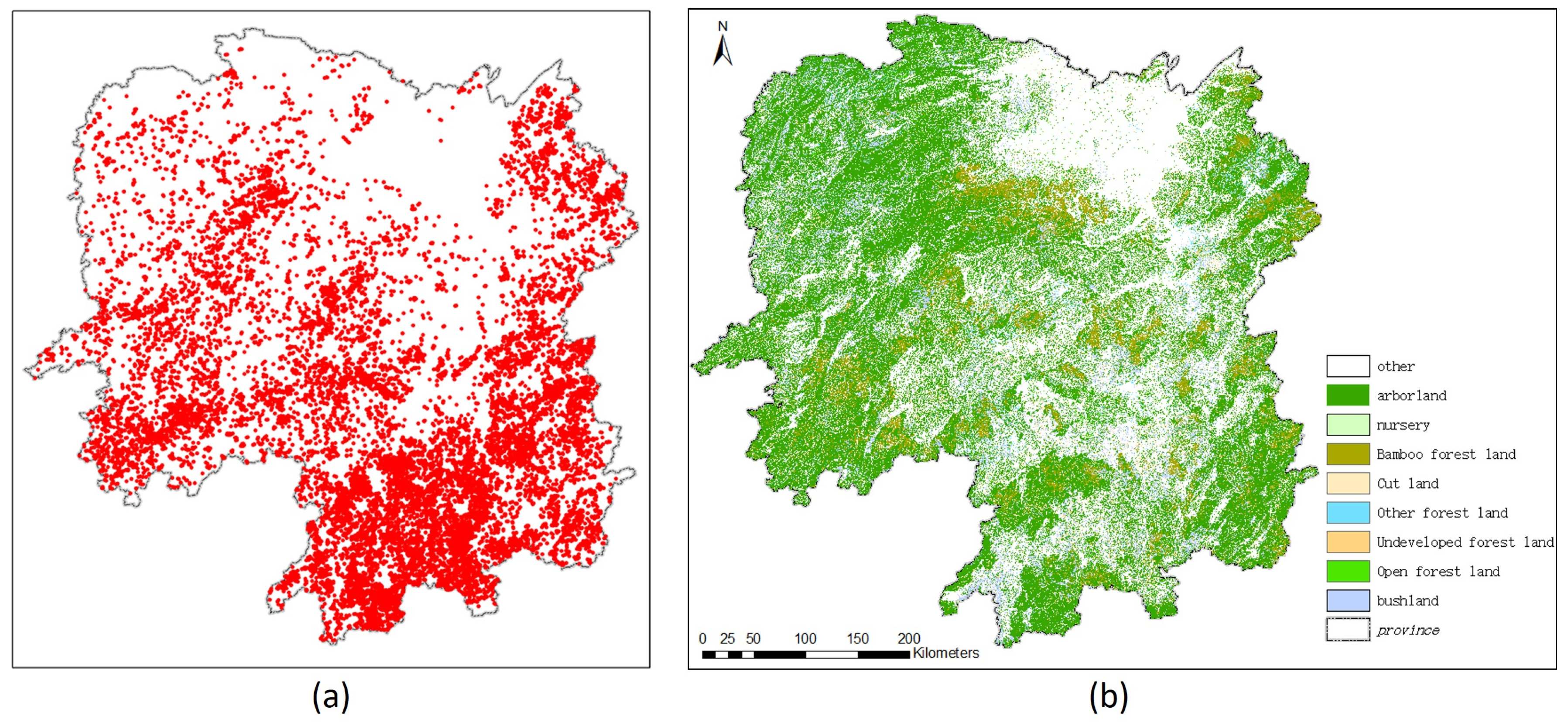
Hunan Province (24°38′–30°08′ N, 108°47′–114°15′ E) is located in south–central China and spans approximately 211,829 km2 (Figure 1). The terrain gradually transitions from low-lying plains in the north, such as the Dongting Lake area, to hilly and mountainous regions in the central and southern parts of the province. Hunan experiences a humid subtropical monsoon climate, characterized by a pronounced dry season from December to February and a wet season from May to August. Forests cover nearly 60% of the province’s land area, with denser vegetation concentrated in the mountainous western and southern zones (Figure 2b). The complex interplay among diverse topography, microclimates, vegetation types, and anthropogenic activities leads to significant spatial heterogeneity in wildfire risk. These characteristics make Hunan a representative region for investigating spatiotemporal wildfire risk under complex environmental and anthropogenic influences.

2.2. Data Collection and Preprocessing

Wildfire records from 2000 to 2024 were obtained from NASA’s Fire Information for Resource Management System (FIRMS), with a spatial resolution of 1 km2. To ensure high data reliability, only wildfire events with a confidence level exceeding 70% were retained, and those occurring in non-forested areas were excluded. This filtering process yielded 18,784 high-confidence wildfire records (Figure 2a).
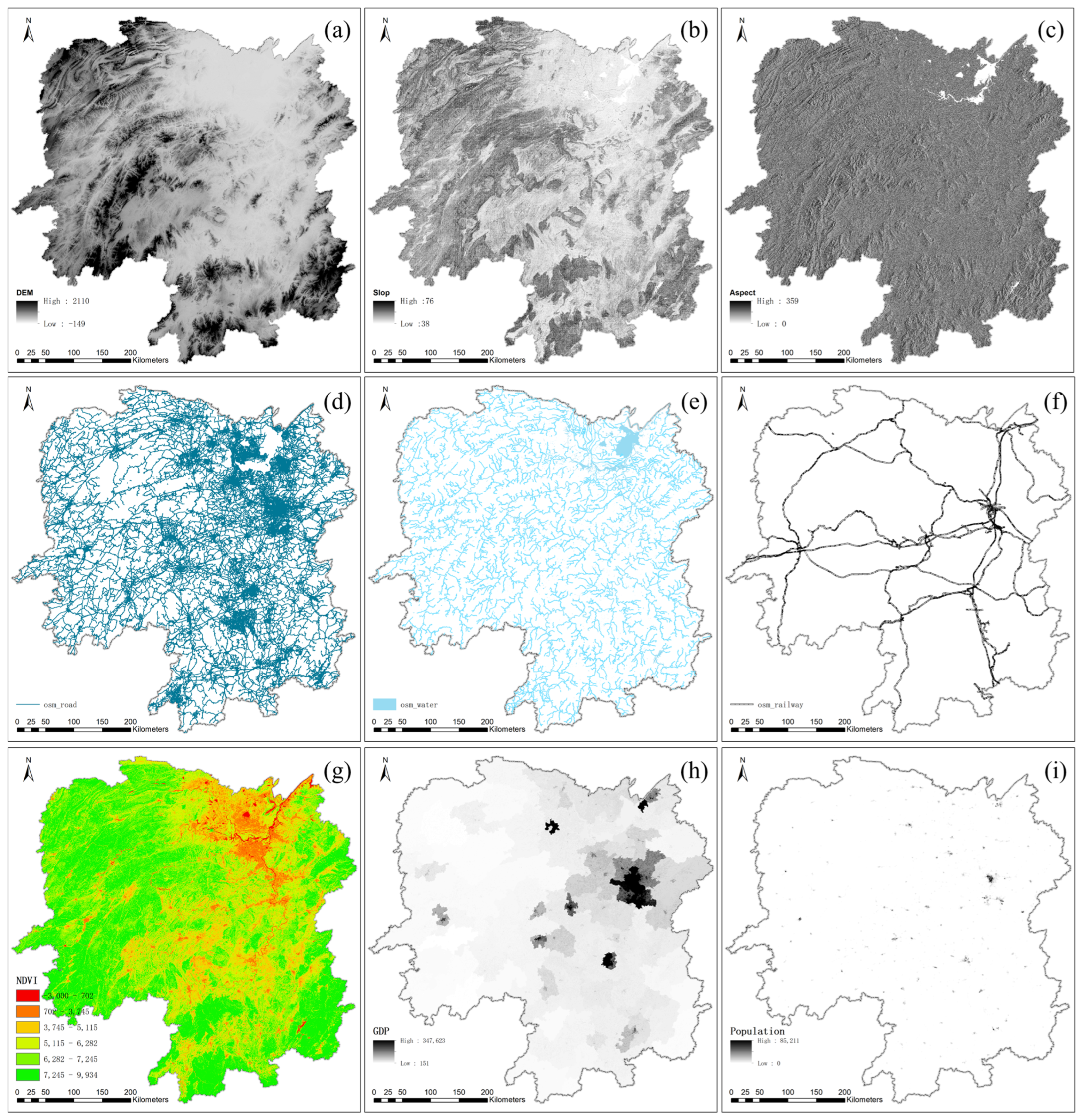
Based on prior studies, 18 explanatory variables were selected to represent meteorological, topographic, vegetation, infrastructure, and socioeconomic drivers of wildfire occurrence (Figure 3 and Table 1). These variables were chosen based on their documented relevance to wildfire occurrence and availability across the study region. Data were obtained from publicly available remote sensing and national statistical sources. All variables were resampled to a uniform 1 km grid to ensure spatial consistency. Missing values were addressed using inverse distance weighted (IDW) interpolation and temporal averaging, ensuring a complete and harmonized dataset for modeling.

3. Methodology

3.1. Research Process

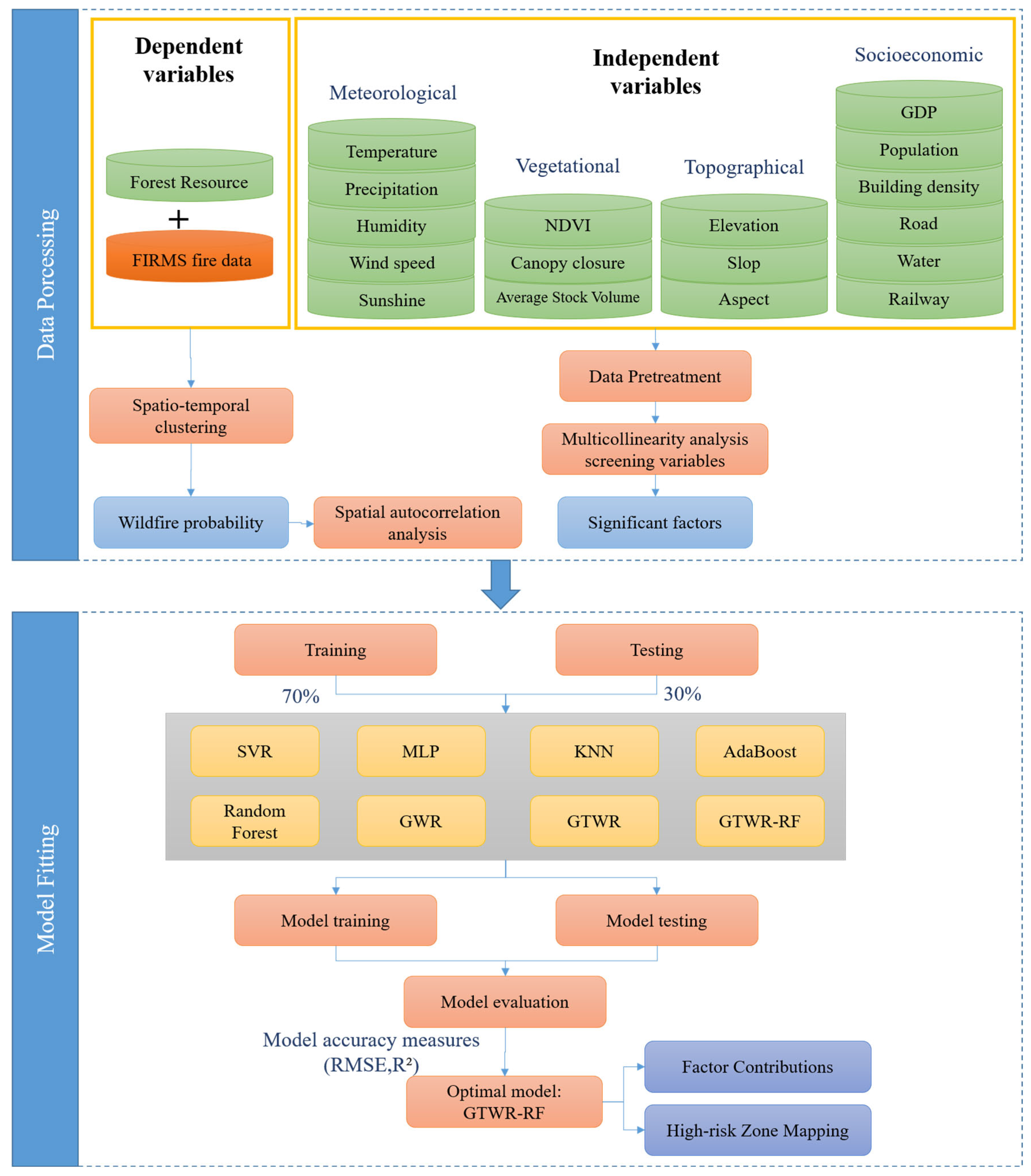
The research framework integrates data pre-processing, variable selection, spatiotemporal clustering, and model training to assess wildfire risk in Hunan Province. The complete research workflow is illustrated in Figure 4.
Following data filtering, ST-DBSCAN was applied to identify spatiotemporal clusters of wildfire events and to derive wildfire occurrence probabilities. Environmental variables were subsequently extracted to each wildfire event to construct the model input dataset. All variables were standardized to improve computational stability and model convergence. Spatial autocorrelation analysis was performed to examine underlying spatial patterns, and multicollinearity among explanatory variables was addressed using the Variance Inflation Factor (VIF) analysis.
Eight models were compared in this study: KNN, MLP, SVR, AdaBoost, RFR, GWR, GTWR and GTWR-RFR. To ensure optimal performance and comparability, each model was tuned using grid search and cross-validation. KNN models were optimized by varying the number of neighbors (K); RF and AdaBoost by adjusting tree depth, estimators, and learning rate; MLP by tuning hidden layers, learning rate, and activation function; and SVR by selecting kernel types and adjusting penalty (C) and kernel coefficient (γ). For spatial models, the GWR bandwidth was selected via cross-validation. GTWR, GTWR-RFR required tuning both spatial bandwidth and the temporal scale parameter (μ), with sensitivity analysis conducted over μ values from 0.1 to 0.9 to evaluate model stability and fit. Model performance was evaluated using RMSE and R2. GTWR-RFR achieved the lowest RMSE and highest R2, and was thus selected as the optimal model. Finally, IDW interpolation was used to visualize the spatial distribution of predicted wildfire probabilities and support subsequent spatial pattern analysis.

3.2. Estimating Wildfire Probability via Spatiotemporal Clustering

To estimate wildfire occurrence probability, this study employed the ST-DBSCAN algorithm, which extends traditional DBSCAN by incorporating both spatial and temporal proximity, without requiring prior specification of the number of clusters [18,22]. For each wildfire event e i , its spatiotemporal neighborhood is defined by events within a spatial radius ( ϵ s ) and a temporal window ( ϵ t ). If the number of events in this neighborhood meets or exceeds a minimum density threshold (MinPts), e i is considered a core point of a cluster. The wildfire probability P i at e i is then calculated by normalizing its neighborhood density against the maximum density observed across all events:
P i = | N ( ϵ s , ϵ t ) ( e i ) | m a x e D | N ( ϵ s , ϵ t ) ( e ) |
This normalization yields a relative spatiotemporal density scaled between 0 and 1, representing the likelihood of wildfire occurrence. Clustering validity was assessed using the Silhouette Coefficient [23].

3.3. Geographically and Temporally Weighted Random Forest Regression and Evaluation Metrics

The GTWR-RFR model synergistically integrates the adaptive spatiotemporal weighting of GTWR with the robust nonlinear learning capability of RF [14]. While GTWR effectively captures spatiotemporal heterogeneity by allowing coefficients to vary across space and time [24], its linear formulation is sensitive to outliers and incapable of modeling complex nonlinear relationships [11,25]. Conversely, standard Random Forest regression (RFR), though robust and non-parametric, inherently lacks mechanisms to account for spatial and temporal dependencies. GTWR-RFR addresses these limitations by training localized RFR models at each spatial location, weighted according to spatiotemporal proximity. The GTWR model at a spatiotemporal point u i , v i , t i is defined as follows:
Y i = β 0 u i , v i , t i + k = 1 p β k u i , v i , t i X i k + ε i , i = 1,2 , n
where β k u i , v i , t i are the location- and time-specific coefficients, and ε i ~ N ( 0 , σ 2 ) are random error term. The coefficients are estimated using weighted least squares:
β ^ = ( X T W i X ) 1 X T W i Y
here W i = d i a g ( w i 0 , w i 1 , w i 2 , , w i n ) is the spatotemporal weight matrix defined by a Gaussian kernel. The weight w i j between observations i and j is determined by their spatiotemporal distance, calculated as follows:
d i j S T = λ u i u j 2 + v i v j 2 + μ ( t i t j ) 2
The corresponding spatiotemporal Gaussian weight function [26] is as follows:
w i j S T = exp ( d i j S T ) 2 h 2 = e x p λ u i u j 2 + v i v j 2 + μ t i t j 2 h 2
where h is the bandwidth, and λ, μ are scale parameters balancing spatial and temporal influences. The optimal bandwidth h is selected by minimizing the corrected Akaike Information Criterion (AICc).
The spatiotemporal weights from GTWR are used to train local RFR models. The final prediction y ^ i at location iis the average output of all M decision trees in the local forest, incorporating the GTWR-derived coefficients as features:
y ^ i = 1 M m = 1 M f m ( β 0 * , β 1 * , , β p * , X i )
where f m () is the prediction function of the m-th tree, β p * are the spatiotemporal coefficients from GTWR, and X i is the vector of explanatory variables at i.
Model performance was evaluated using four standard metrics, including RMSE, MAE, R2, and AICc. Lower RMSE and MAE indicate better prediction accuracy, while higher R2 reflects stronger explanatory power.

4. Results

4.1. Spatial Characteristics and Feature Selection

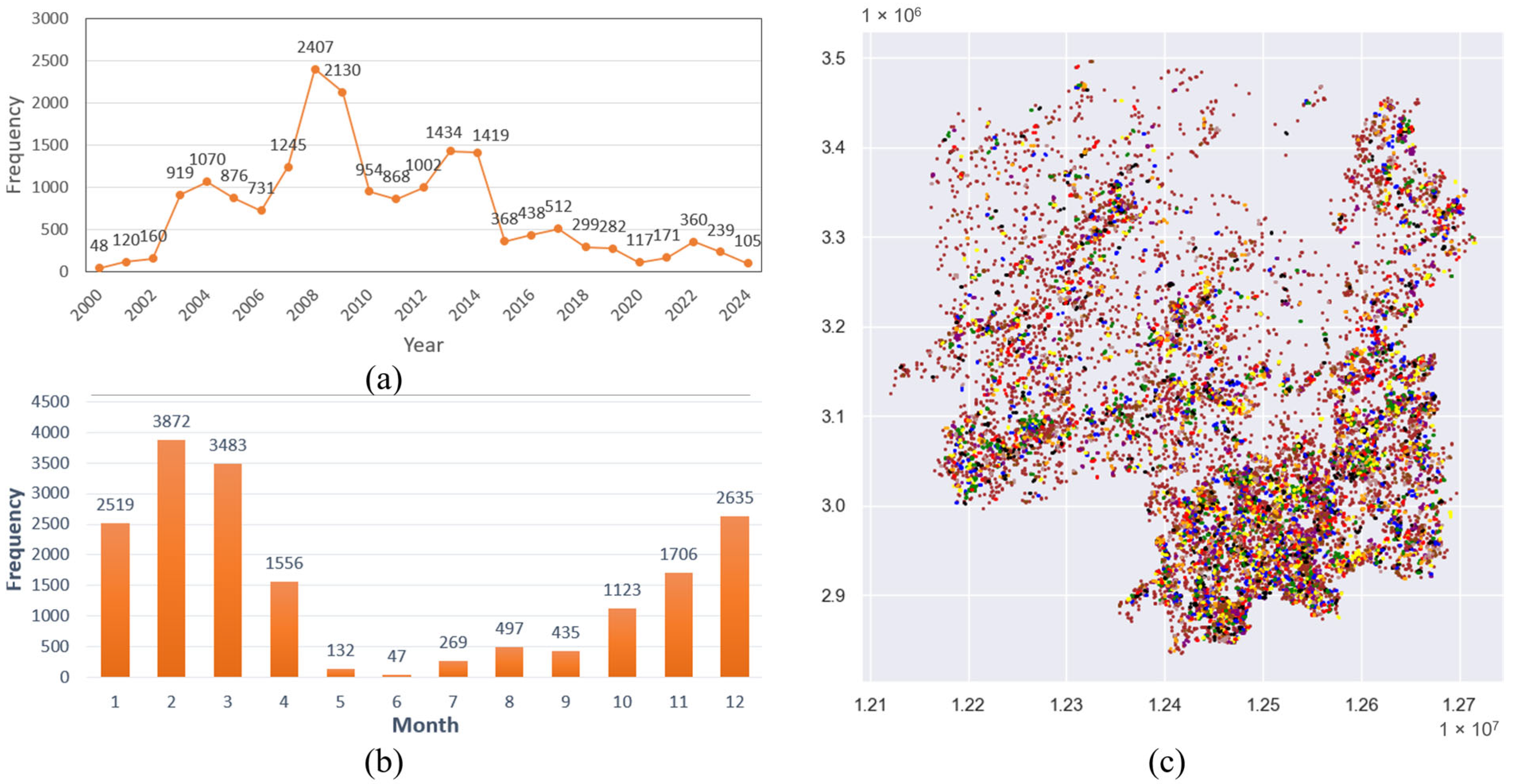
Wildfire events in Hunan Province exhibit distinct temporal and spatial heterogeneity. The annual frequency of wildfires rose steadily from 2000 to 2008, followed by a declining trend (Figure 5a). Seasonally, two major wildfire seasons are observed annually, peaking between January–April and October–December (Figure 5b). February records the highest frequency, driven by dry conditions, intermittent winds, and human activities such as traditional festivals. Conversely, wildfire activity is minimal from May to September, when plum rains and summer monsoons elevate vegetation moisture.
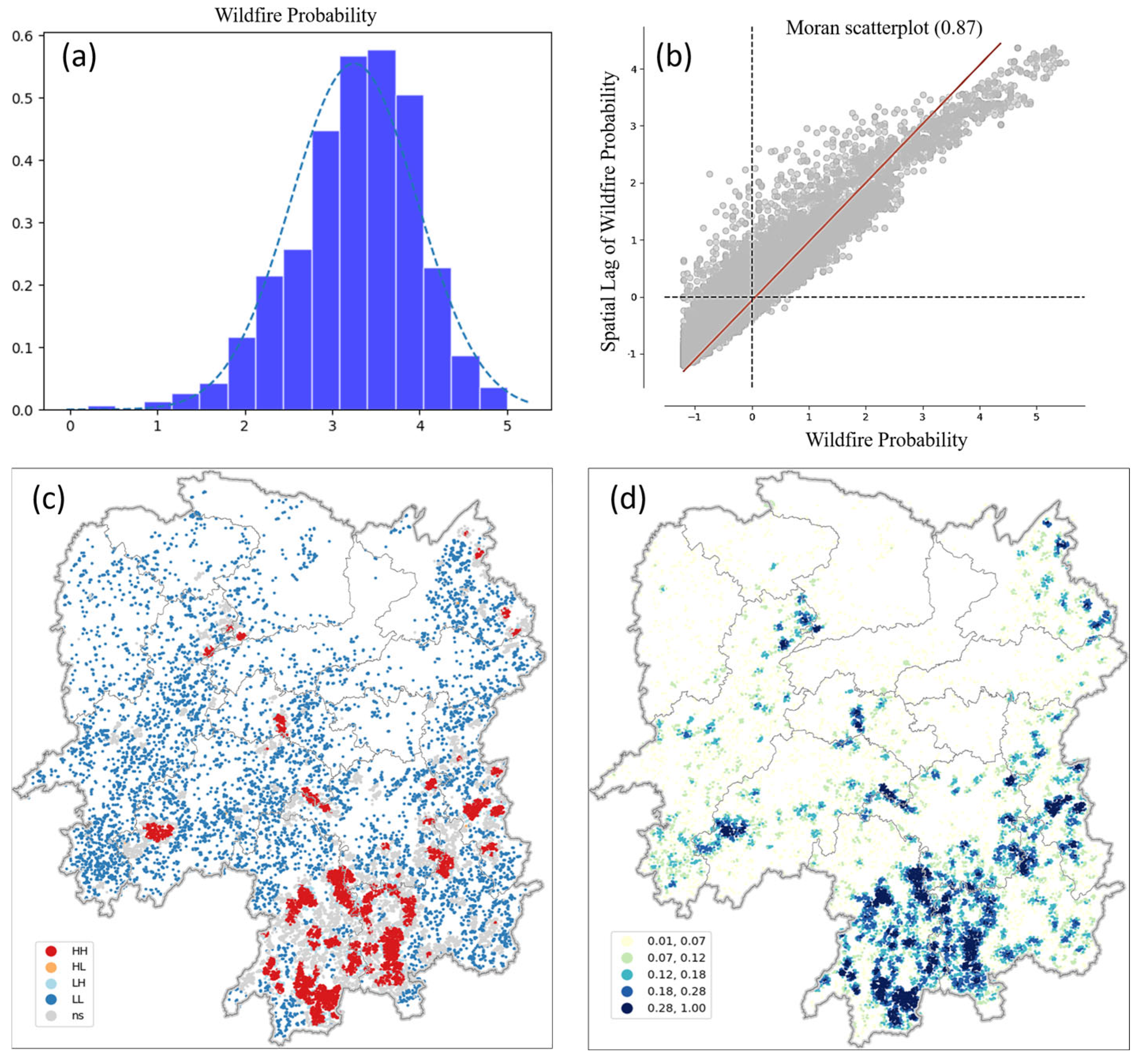
Using a 5 km spatial radius and a 3-day temporal window, ST-DBSCAN identified 3347 high-density wildfire clusters, while 29.03% of events were classified as noise, indicating isolated low-risk occurrences. Wildfire occurrence probabilities were then computed for each event based on its cluster (Figure 5c). The log-transformed wildfire occurrence probability exhibits a distribution close to normality (Figure 6a).
Global Moran’s I (0.87; Z = 306.8) confirms strong positive spatial autocorrelation (Figure 6b). Local Indicators of Spatial Association (LISA) further reveal a clear north–south gradient in wildfire occurrence: hotspots concentrate in southern and south-eastern Hunan, whereas coldspots dominate the north and central regions (Figure 6c,d). This significant positive spatial autocorrelation underscores the need for models that incorporate spatial heterogeneity.
To ensure reliable model inputs, multicollinearity among explanatory variables was assessed via variance inflation factor (VIF) analysis [27]. Factors with VIF values between 2.04 and 5.99 were retained (Table 2), satisfying VIF < 10 and tolerance > 0.1 criteria [28,29]. The final set of 13 variables captures the principal climatic, topographic, vegetative, and anthropogenic determinants of wildfire risk.

4.2. Model Performance Evaluation

We evaluated eight models, including five machine learning algorithms (KNN, SVR, MLP, AdaBoost, RFR) and three spatial regression techniques (GWR, GTWR, GTWR-RFR), for wildfire probability prediction. Table 3 summarized the performance metrics of all models. The pronounced performance disparities among these models can be primarily attributed to their inherent capacities for handling spatial heterogeneity and nonlinear relationships. Predicted versus observed probabilities are shown in scatterplots (Figure 7). Among the machine learning methods, RFR achieved the best performance (R2 = 0.802; RMSE = 0.6609), whereas KNN performed the poorest (R2 = 0.376; RMSE = 0.8635). The superior performance of RFR is attributed to its ensemble structure and intrinsic capability to model complex nonlinear interactions without a priori assumptions. In contrast, the poor performance of KNN likely stems from the curse of dimensionality, which impairs its ability to discern meaningful patterns in high-dimensional feature space [30].
To account for spatial heterogeneity, GWR was fitted using a fixed Gaussian kernel with a bandwidth of 7 639 m, yielding R2 = 0.848 and RMSE = 0.3899 (Figure 7f). Incorporating temporal heterogeneity, the GTWR model applied the same spatial bandwidth and a temporal decay parameter (μ = 0.2), improving model performance to R2 = 0.885 and RMSE = 0.3387 (Figure 7g). The improvement from GWR to GTWR highlights the importance of addressing temporal non-stationarity alongside spatial variation. GTWR’s adaptive spatiotemporal weighting dynamically adjusts local fits based on proximity in both space and time, effectively representing non-stationary relationships in wildfire drivers [24]. The hybrid GTWR-RFR model was then developed by integrating RFR into the GTWR framework. By combining RF’s nonlinear learning and feature selection capabilities with GTWR’s adaptive spatiotemporal weighting, GTWR-RFR achieved superior predictive accuracy, with R2 = 0.969 and RMSE = 0.1743 (Figure 7h). This integration enables the model to capture complex nonlinear wildfire patterns more effectively [31,32]. By leveraging spatially and temporally localized learning, GTWR-RFR effectively resolves the limitations associated with global-stationarity assumptions in conventional machine learning models while overcoming the linear constraints of standard spatial regression approaches.
We applied Global Moran’s I to analyze the spatial autocorrelation of prediction residuals across all models to assess whether the models effectively captured spatial heterogeneity [16,33]. Table 4 summarizes the Moran’s I results. Residual clustering is evident in non-spatial models, with Moran’s I exceeding 0.5. In contrast, GTWR-RFR achieved the lowest value (0.2462), indicating minimal residual autocorrelation and superior spatial generalization. The analysis of residual spatial autocorrelation further quantifies the uncertainty associated with ignoring spatial effects, which signifies unexplained spatial structure and potential model misspecification.

4.3. Spatial Patterns of Coefficient Estimates

Statistical analysis on the GTWR-RFR coefficient estimates is summarized in Table 5, and most coefficient means are near zero, indicating that local rather than global factors predominantly govern wildfire risk. The standard deviation (STD) of each coefficient quantifies spatial variability: lower STD values (e.g., CC, STD = 0.021) denote consistent influences across Hunan, whereas higher STD values (e.g., GDP, STD = 0.117) reflect substantial local variation in driver effects.
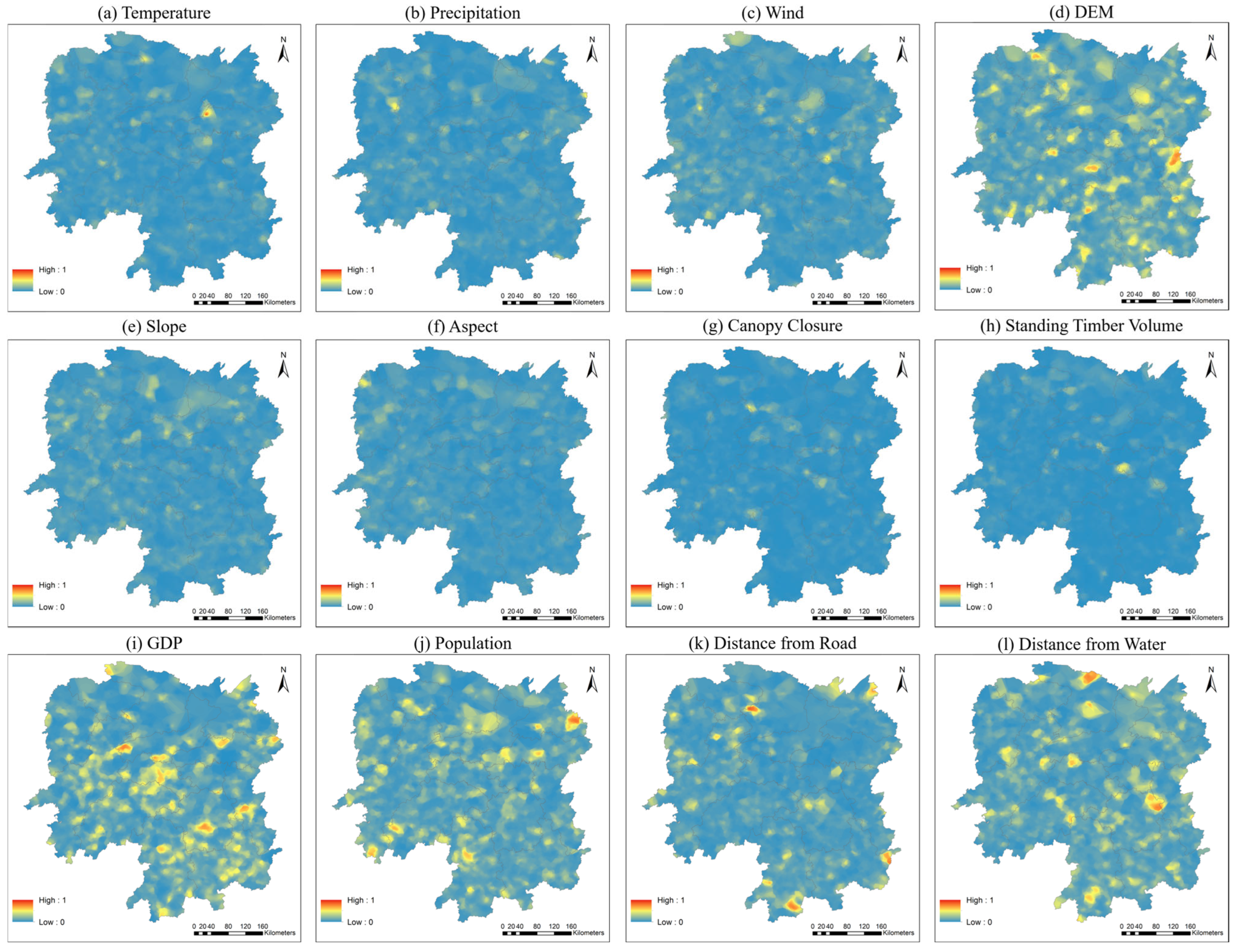
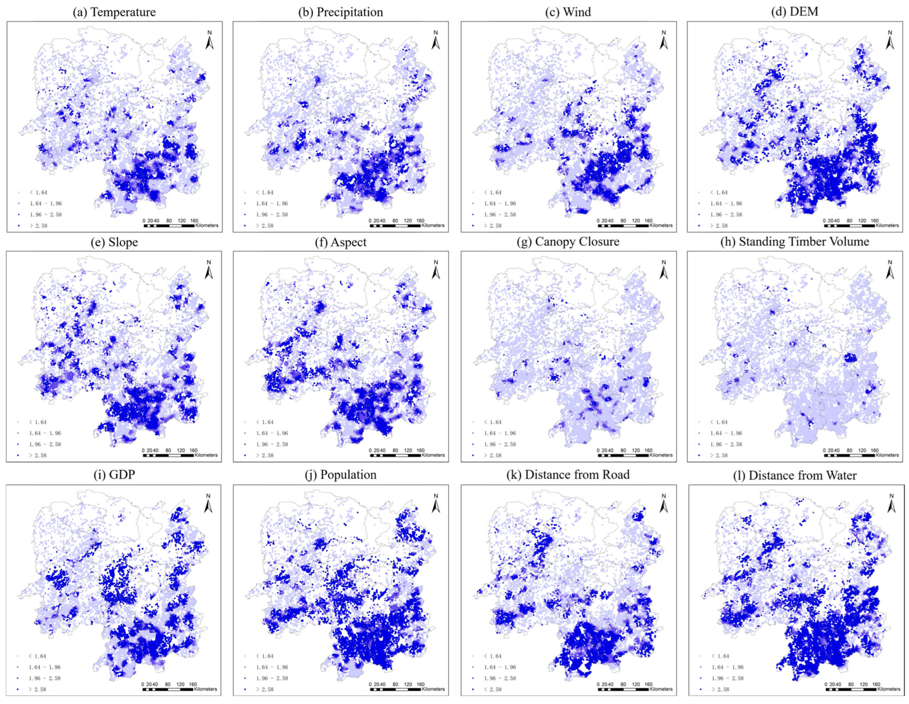
Figure 8 and Figure 9 present IDW-interpolated maps of local variable importance and corresponding t-value distributions, respectively, highlighting spatial heterogeneity in driver impacts on wildfire probability. Among all factors, DEM, GDP, population density, distance to roads, and distance to water bodies emerge as especially influential. DEM governs microclimatic conditions and vegetation distribution, thereby affecting fuel availability and dryness [34,35,36]. Regional GDP reflects economic disparities that shape infrastructure and wildfire prevention investments, with spatial heterogeneity in GDP driving variation in ignition sources and suppression capacity [37]. High population density contributes to forest fragmentation and increased edge effects, thereby elevating wildfire susceptibility [38]. Greater distance from roads correlates with higher risk due to delayed fire-fighting response [39], while increased distance from water bodies corresponds to elevated risk, as water features serve as natural firebreaks [40]. Collectively, these drivers interact through ecological and socioeconomic pathways to shape the complex spatial patterns of wildfire occurrence. These spatially heterogeneous coefficients offer valuable insights for tailoring region-specific wildfire prevention strategies.

4.4. Risk Classification and Spatial Distribution

Based on GTWR-RFR results, wildfire risk in Hunan Province was categorized into four levels (Table 6). The spatial distribution reveals a southeast-to-northwest decreasing gradient (Figure 10), aligning with prior studies [41,42]. This pattern reflects the combined influence of topography, climate, vegetation, and human activities on wildfire occurrence, especially in rugged, densely forested terrain with frequent anthropogenic disturbances [43,44]. In the northern and western regions, such as the Dongting Lake basin and the western highlands, wildfire risk remains low due to sparse vegetation, high precipitation, limited fuel, and reduced human disturbance associated with elevation and remoteness. In contrast, high-risk zones are concentrated in the south-eastern, central, and southern regions. The combination of dense vegetation, abundant fuels, high population density, and well-developed road accessibility in these areas significantly elevates the risk of wildfires [45]. Moreover, complex terrain and monsoonal winds in the south-eastern mountains further exacerbate wildfire susceptibility [46,47].
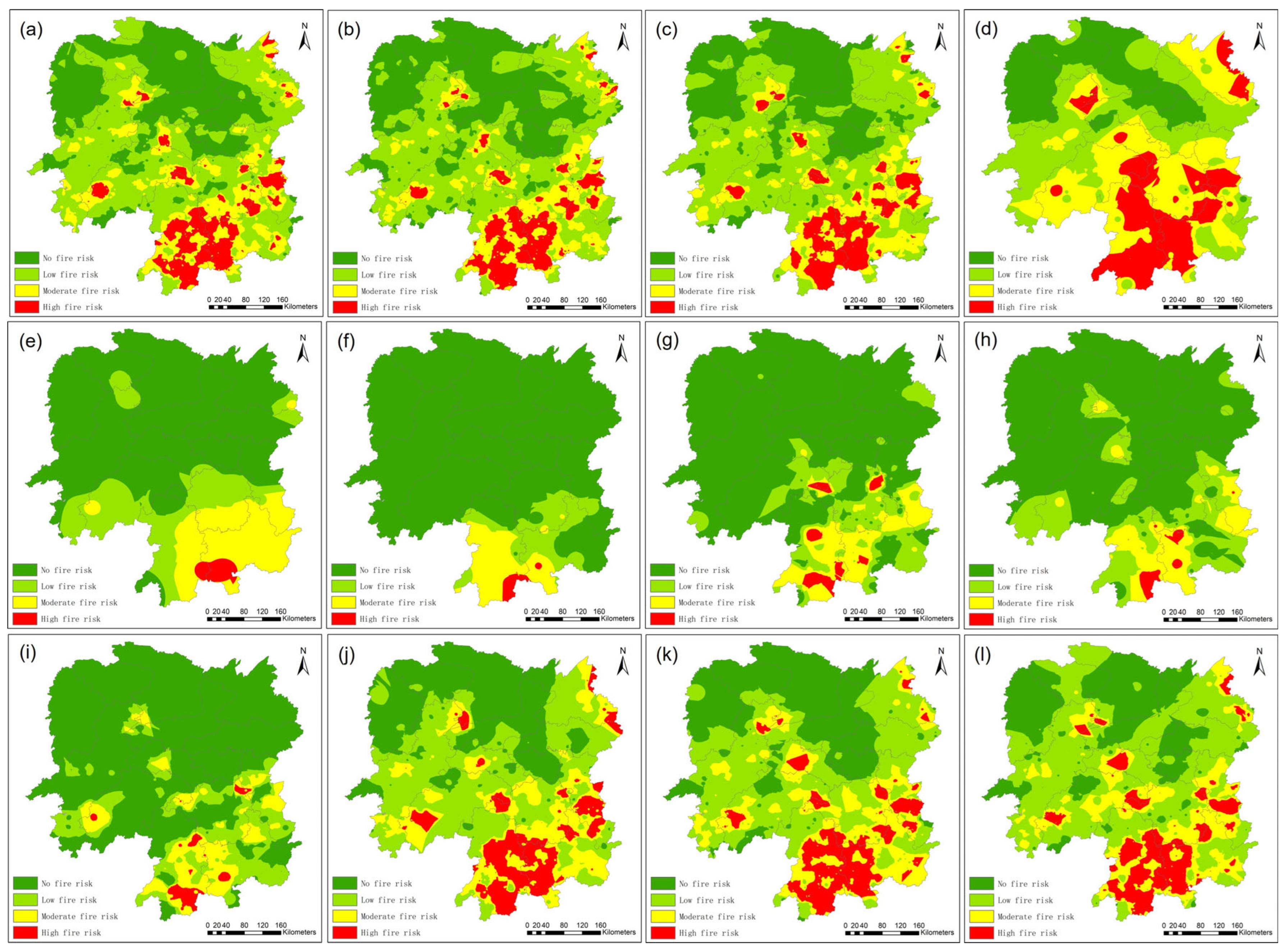
We employed the GTWR-RFR model to generate monthly wildfire risk predictions for Hunan Province, China, revealing distinct and pronounced seasonal variability patterns. The monthly risk maps (Figure 11) clearly illustrate this regularity. High-risk periods occur from January to April and October to December. Winter–spring months (January–March) feature low precipitation and fuel desiccation, particularly in southern and eastern Hunan, with April peaking due to Qingming Festival burning activities. By contrast, May–September shows low risk despite high temperatures, as monsoonal rains maintain high fuel moisture. Risk rebounds in October–December as rainfall wanes and agricultural burning resumes. These findings highlight the necessity of seasonally targeted prevention measures, especially limiting human ignitions, raising public awareness, enhancing wildfire monitoring and optimizing resource deployment, during peak wildfire seasons.

5. Discussion

5.1. Advantages of Probability-Based Wildfire Modeling via ST-DBSCAN

Traditional wildfire risk models typically adopt a binary fire–nonfire classification framework, which often requires artificially generated non-fire samples. These samples tend to share similar environmental characteristics with fire-prone areas, such as climate, topography, vegetation, and human activity, thereby introducing bias [48]. Moreover, binary classification fails to capture the spatially coherent nature of wildfire risk [49,50].
To overcome these limitations, this study employs a probability-based modeling framework. Wildfire probability is estimated from the density of historical wildfire clusters, which are effectively identified by ST-DBSCAN based on spatial and temporal proximity, allowing the distinction between fire-prone areas and isolated occurrences [18,51]. The probability-based framework offers several advantages: (1) Reduces sampling bias by avoiding randomly generated non-fire samples; (2) Preserves spatiotemporal patterns of wildfire occurrence, enabling more interpretable modeling; and (3) Improves data quality by filtering noise and outliers through clustering. This probability-based approach lays a robust foundation for downstream spatial modeling, facilitating improved generalization and interpretability.

5.2. Strengths of the GTWR-RFR Hybrid Regression

Because wildfire probability exhibits strong spatial autocorrelation, adaptive models with spatially varying coefficients are required [52,53]. GTWR-RFR integrates the nonlinear learning capability of RFR with the spatiotemporal weighting mechanism of GTWR, thereby addressing the limitations of both linear spatial models (e.g., sensitivity to outliers) and non-spatial models (e.g., neglect of spatial variation) [54]. By calibrating local parameters based on spatiotemporal proximity, this approach flexibly adjusts weights [10,55], thereby more effectively capturing region-specific variations in key wildfire drivers (e.g., DEM, GDP, population density, distance to roads and water bodies) while retaining model interpretability [24].
GTWR-RFR enhances wildfire risk prediction by capturing both spatial heterogeneity and nonlinearity. Our results demonstrate that it outperforms both non-spatial machine learning algorithms and traditional spatial regression models, achieving superior model fit, the lowest error, and the smallest residual, indicating the highest predictive accuracy and minimized spatial bias. The strong agreement between predicted and observed values validates the model’s robustness. These strengths establish GTWR-RFR as a robust and interpretable framework for capturing dynamic wildfire patterns in heterogeneous environments.

5.3. Limitations and Future Directions

Although the GTWR-RFR framework demonstrates significant advantages in modeling complex spatiotemporal wildfire risk, several limitations remain. First, the model involves high computational complexity. GTWR requires constructing a local weight matrix and estimating regression coefficients for each spatiotemporal sample, while the RF relies on extensive ensemble operations. Second, the model’s performance is sensitive to data quality. Spatially or temporally uneven data distribution may induce local overfitting in the regional RF models, thereby compromising predictive reliability. Finally, the framework’s performance is sensitive to parameterization. Suboptimal spatiotemporal thresholds in ST-DBSCAN or inappropriate RF hyperparameters may induce instability and degrade accuracy [23,56]. Model generalization may be limited by regional or temporal heterogeneity, reducing transferability across study areas.
Future work should prioritize enhancing the model’s computational efficiency, generalization capability, and predictive accuracy. Developing parallel and distributed computing strategies to accelerate processing; exploring alternative regressors such as local Support Vector Machines (SVMs) or neural networks to further increase flexibility and predictive performance; and incorporating high-resolution and spatiotemporally consistent variables (e.g., fuel moisture, fuel load, and fine-scale socioeconomic indicators) to refine model realism.

6. Conclusions

This study developed an integrated spatiotemporal framework combining ST-DBSCAN clustering with GTWR-RFR for wildfire risk prediction. The model significantly improves predictive accuracy by leveraging RF’s nonlinear modeling capability and GTWR’s adaptive spatiotemporal weighting, while also eliminating the bias in artificially generated non-fire samples through density-based probability estimation. Applied to Hunan Province, the framework reveals pronounced spatiotemporal heterogeneity in key wildfire risk drivers. The resulting risk maps and the spatiotemporal heterogeneity of key drivers provide actionable insights for optimizing resource allocation and targeted prevention strategies. Future research should focus on enhancing computational efficiency through parallel and distributed computing, improving predictive flexibility via alternative regressors such as local SVM or neural networks, and extending the framework to diverse geographic regions and climate scenarios to maximize its applicability in wildfire management and early warning systems.

Author Contributions

S.X.: Writing—review and editing, writing—original draft, methodology, investigation, data curation, resources, conceptualization; H.X. (Huashun Xiao): Writing—review and editing, resources, methodology, conceptualization, formal analysis, funding acquisition; G.Z.: Methodology, resources, conceptualization; H.X. (Haizhou Xu): Methodology, data curation. All authors have read and agreed to the published version of the manuscript.

Funding

This research was funded by project from Hunan Forestry Science and Technology Research and Innovation Project (No. XLKY202331) and project from Scientific Research Fund of Hunan Provincial Education Department (No. 22A0192).

Data Availability Statement

Source code and data at https://github.com/xsfnew/GTWR_RFR (accessed on 21 October 2025). Detailed documentation for application installation, testing, and deployment can be found at https://github.com/xsfnew/GTWR_RFR/blob/master/README.md (accessed on 21 October 2025).

Acknowledgments

During the preparation of this work the authors used ChatGPT-4o in order to improve the readability and refine language. After using this tool/service, the authors reviewed and edited the content as needed and take full responsibility for the content of the publication.

Conflicts of Interest

The authors declare no conflicts of interest.

References

  1. Walker, X.J.; Baltzer, J.L.; Cumming, S.G.; Day, N.J.; Ebert, C.; Goetz, S.; Johnstone, J.F.; Potter, S.; Rogers, B.M.; Schuur, E.A.G.; et al. Increasing wildfires threaten historic carbon sink of boreal forest soils. Nature 2019, 572, 520–523. [Google Scholar] [CrossRef] [PubMed]
  2. Modugno, S.; Balzter, H.; Cole, B.; Borrelli, P. Mapping regional patterns of large forest fires in Wildland-Urban Interface areas in Europe. J. Environ. Manag. 2016, 172, 112–126. [Google Scholar] [CrossRef]
  3. Guo, H.F.; Yu, W. Study weather grade prediction model of forest-fire risk in Hunan province. J. Cent. South Univ. For. Technol. 2016, 36, 44–47. [Google Scholar]
  4. Su, Z.; Zheng, L.; Luo, S.; Tigabu, M.; Guo, F. Modeling wildfire drivers in Chinese tropical forest ecosystems using global logistic regression and geographically weighted logistic regression. Nat. Hazards 2021, 108, 1317–1345. [Google Scholar] [CrossRef]
  5. Ma, W.; Feng, Z.; Cheng, Z.; Chen, S.; Wang, F. Identifying Forest Fire Driving Factors and Related Impacts in China Using Random Forest Algorithm. Forests 2020, 11, 507. [Google Scholar] [CrossRef]
  6. Gigović, L.; Pourghasemi, H.R.; Drobnjak, S.; Bai, S. Testing a New Ensemble Model Based on SVM and Random Forest in Forest Fire Susceptibility Assessment and Its Mapping in Serbia’s Tara National Park. Forests 2019, 10, 408. [Google Scholar] [CrossRef]
  7. Chen, F.; Du, Y.; Niu, S.; Zhao, J. Modeling Forest Lightning Fire Occurrence in the Daxinganling Mountains of Northeastern China with MAXENT. Forests 2015, 6, 1422–1438. [Google Scholar] [CrossRef]
  8. Liang, H; Wang, W.; Guo, F.; Lin, F.; Lin, X. Comparing the application of logistic and geographically weighted logistic regression models for Fujian forest fire forecasting. Acta Ecol. Sin. 2017, 37, 399–406. [Google Scholar] [CrossRef]
  9. Zhang, X.; Lan, M.; Ming, J.; Zhu, J.; Lo, S. Spatiotemporal Heterogeneity of Forest Fire Occurrence Based on Remote Sensing Data: An Analysis in Anhui, China. Remote Sens. 2023, 15, 598. [Google Scholar] [CrossRef]
  10. Pahlavani, P.; Raei, A.; Bigdeli, B.; Ghorbanzadeh, O. Identifying Influential Spatial Drivers of Forest Fires through Geographically and Temporally Weighted Regression Coupled with a Continuous Invasive Weed Optimization Algorithm. Fire 2024, 7, 33. [Google Scholar] [CrossRef]
  11. Santos, F.; Graw, V.; Bonilla, S. A geographically weighted random forest approach for evaluate forest change drivers in the Northern Ecuadorian Amazon. PLoS ONE 2019, 14, e0226224. [Google Scholar] [CrossRef] [PubMed]
  12. Li, W.; Ni, L.; Li, Z.-L.; Duan, S.-B.; Wu, H. Evaluation of Machine Learning Algorithms in Spatial Downscaling of MODIS Land Surface Temperature. IEEE J. Sel. Top. Appl. Earth Obs. Remote Sens. 2019, 12, 2299–2307. [Google Scholar] [CrossRef]
  13. Yin, Z.; Ding, J.; Liu, Y.; Wang, R.; Wang, Y.; Chen, Y.; Qi, J.; Wu, S.; Du, Z. GNNWR: An open-source package of spatiotemporal intelligent regression methods for modeling spatial and temporal nonstationarity. Geosci. Model Dev. 2024, 17, 8455–8468. [Google Scholar] [CrossRef]
  14. Georganos, S.; Grippa, T.; Niang Gadiaga, A.; Linard, C.; Lennert, M.; Vanhuysse, S.; Mboga, N.; Wolff, E.; Kalogirou, S. Geographical random forests: A spatial extension of the random forest algorithm to address spatial heterogeneity in remote sensing and population modelling. Geocarto Int. 2019, 36, 121–136. [Google Scholar] [CrossRef]
  15. Du, Z.; Wang, Z.; Wu, S.; Zhang, F.; Liu, R. Geographically neural network weighted regression for the accurate estimation of spatial non-stationarity. Int. J. Geogr. Inf. Sci. 2020, 34, 1353–1377. [Google Scholar] [CrossRef]
  16. Khan, S.N.; Li, D.; Maimaitijiang, M. A Geographically Weighted Random Forest Approach to Predict Corn Yield in the US Corn Belt. Remote Sens. 2022, 14, 2843. [Google Scholar] [CrossRef]
  17. Fayaz, J.; Galasso, C. Interpretability and spatial efficacy of a deep-learning-based on-site early warning framework using explainable artificial intelligence and geographically weighted random forests. Geosci. Front. 2024, 15, 101839. [Google Scholar] [CrossRef]
  18. Birant, D.; Kut, A. ST-DBSCAN: An algorithm for clustering spatial–temporal data. Data Knowl. Eng. 2007, 60, 208–221. [Google Scholar] [CrossRef]
  19. Su, H.; Ma, X.; Li, M. An improved spatio-temporal clustering method for extracting fire footprints based on MCD64A1 in the Daxing’anling Area of north-eastern China. Int. J. Wildland Fire 2023, 32, 679–693. [Google Scholar] [CrossRef]
  20. Son, M.-W.; Kim, C.-G.; Kim, B.-S. Development of an Algorithm for Assessing the Scope of Large Forest Fire Using VIIRS-Based Data and Machine Learning. Remote Sens. 2024, 16, 2667. [Google Scholar] [CrossRef]
  21. Ahajjam, A.; Allgaier, M.; Chance, R.; Chukwuemeka, E.; Putkonen, J.; Pasch, T. Enhancing prediction of wildfire occurrence and behavior in Alaska using spatio-temporal clustering and ensemble machine learning. Ecol. Inform. 2025, 85, 102963. [Google Scholar] [CrossRef]
  22. Ram, A.; Jalal, S.; Jalal, A.S.; Kumar, M. A Density Based Algorithm for Discovering Density Varied Clusters in Large Spatial Databases. Int. J. Comput. Appl. 2010, 3, 1–4. [Google Scholar] [CrossRef]
  23. Rousseeuw, P.J. Silhouettes: A graphical aid to the interpretation and validation of cluster analysis. J. Comput. Appl. Math. 1987, 20, 53–65. [Google Scholar] [CrossRef]
  24. Fotheringham, A.S.; Crespo, R.; Yao, J. Geographical and Temporal Weighted Regression (GTWR). Geogr. Anal. 2015, 47, 431–452. [Google Scholar] [CrossRef]
  25. Schmidt, A.F.; Finan, C. Linear regression and the normality assumption. J. Clin. Epidemiol. 2018, 98, 146–151. [Google Scholar] [CrossRef]
  26. Diniz-Filho, J.A.; Soares, T.N.; de Campos Telles, M.P. Geographically weighted regression as a generalized Wombling to detect barriers to gene flow. Genetica 2016, 144, 425–433. [Google Scholar] [CrossRef] [PubMed]
  27. O’brien, R.M. A Caution Regarding Rules of Thumb for Variance Inflation Factors. Qual. Quant. 2007, 41, 673–690. [Google Scholar] [CrossRef]
  28. Kalantar, B.; Ueda, N.; Idrees, M.O.; Janizadeh, S.; Ahmadi, K.; Shabani, F. Forest Fire Susceptibility Prediction Based on Machine Learning Models with Resampling Algorithms on Remote Sensing Data. Remote Sens. 2020, 12, 3682. [Google Scholar] [CrossRef]
  29. Barreto, J.S.; Armenteras, D. Open Data and Machine Learning to Model the Occurrence of Fire in the Ecoregion of “Llanos Colombo–Venezolanos”. Remote Sens. 2020, 12, 3921. [Google Scholar] [CrossRef]
  30. Weber, R.; Schek, H.-J.; Blott, S. A Quantitative Analysis and Performance Study for Similarity-Search Methods in High-Dimensional Spaces. In Proceedings of the 24rd International Conference on Very Large Data Bases, New York, NY, USA, 24–27 August 1998; pp. 194–205. [Google Scholar]
  31. DeCastro, A.L.; Juliano, T.W.; Kosović, B.; Ebrahimian, H.; Balch, J.K. A Computationally Efficient Method for Updating Fuel Inputs for Wildfire Behavior Models Using Sentinel Imagery and Random Forest Classification. Remote Sens. 2022, 14, 1447. [Google Scholar] [CrossRef]
  32. Van Wyk, J.; du Preez, J.; Versfeld, J. Temporal separation of whale vocalizations from background oceanic noise using a power calculation. Ecol. Inform. 2022, 69, 101627. [Google Scholar] [CrossRef]
  33. Liu, X.; Kounadi, O.; Zurita-Milla, R. Incorporating Spatial Autocorrelation in Machine Learning Models Using Spatial Lag and Eigenvector Spatial Filtering Features. ISPRS Int. J. Geo-Inf. 2022, 11, 242. [Google Scholar] [CrossRef]
  34. Arganaraz, J.P.; Radeloff, V.C.; Bar-Massada, A.; Gavier-Pizarro, G.I.; Scavuzzo, C.M.; Bellis, L.M. Assessing wildfire exposure in the Wildland-Urban Interface area of the mountains of central Argentina. J. Environ. Manag. 2017, 196, 499–510. [Google Scholar] [CrossRef]
  35. Shao, Y.; Feng, Z.; Sun, L.; Yang, X.; Li, Y.; Xu, B.; Chen, Y. Mapping China’s Forest Fire Risks with Machine Learning. Forests 2022, 13, 856. [Google Scholar] [CrossRef]
  36. Koutsias, N.; Martínez-Fernández, J.; Allgöwer, B. Do Factors Causing Wildfires Vary in Space? Evidence from Geographically Weighted Regression. GISci. Remote Sens. 2013, 47, 221–240. [Google Scholar] [CrossRef]
  37. Guo, F.; Wang, G.; Su, Z.; Liang, H.; Wang, W.; Lin, F.; Liu, A. What drives forest fire in Fujian, China? Evidence from logistic regression and Random Forests. Int. J. Wildland Fire 2016, 25, 505–519. [Google Scholar] [CrossRef]
  38. Armenteras, D.; González, T.M.; Retana, J. Forest fragmentation and edge influence on fire occurrence and intensity under different management types in Amazon forests. Biol. Conserv. 2013, 159, 73–79. [Google Scholar] [CrossRef]
  39. Chuvieco, E.; Aguado, I.; Yebra, M.; Nieto, H.; Salas, J.; Martín, M.P.; Vilar, L.; Martínez, J.; Martín, S.; Ibarra, P.; et al. Development of a framework for fire risk assessment using remote sensing and geographic information system technologies. Ecol. Model. 2010, 221, 46–58. [Google Scholar] [CrossRef]
  40. Massetti, A.; Rüdiger, C.; Yebra, M.; Hilton, J. The Vegetation Structure Perpendicular Index (VSPI): A forest condition index for wildfire predictions. Remote Sens. Environ. 2019, 224, 167–181. [Google Scholar] [CrossRef]
  41. Wang, S.; Zhang, G.; Tan, S.Q.; Wang, P.; Wu, X. Assessment of forest fire risk in Hunan province based on spatial logistic model Technol. J. Cent. South Univ. For. Technol. 2020, 40, 88–95. [Google Scholar]
  42. Tan, C.; Feng, Z. Mapping Forest Fire Risk Zones Using Machine Learning Algorithms in Hunan Province, China. Sustainable 2023, 15, 6292. [Google Scholar] [CrossRef]
  43. Li, W.; Xu, Q.; Yi, J.; Liu, J. Predictive model of spatial scale of forest fire driving factors: A case study of Yunnan Province, China. Sci. Rep. 2022, 12, 19029. [Google Scholar] [CrossRef] [PubMed]
  44. Tian, Y.; Wu, Z.; Cui, S.; Hong, W.; Wang, B.; Li, M. Assessing wildfire susceptibility and spatial patterns in diverse forest ecosystems across China: An integrated geospatial analysis. J. Clean. Prod. 2025, 490, 144800. [Google Scholar] [CrossRef]
  45. Yang, X.; Jin, X.; Zhou, Y. Wildfire Risk Assessment and Zoning by Integrating Maxent and GIS in Hunan Province, China. Forests 2021, 12, 1299. [Google Scholar] [CrossRef]
  46. Wu, Z.; He, H.S.; Yang, J.; Liu, Z.; Liang, Y. Relative effects of climatic and local factors on fire occurrence in boreal forest landscapes of northeastern China. Sci. Total Environ. 2014, 493, 472–480. [Google Scholar] [CrossRef]
  47. Guo, F.; Su, Z.; Wang, G.; Sun, L.; Tigabu, M.; Yang, X.; Hu, H. Understanding fire drivers and relative impacts in different Chinese forest ecosystems. Sci. Total Environ. 2017, 605–606, 411–425. [Google Scholar] [CrossRef]
  48. Parisien, M.-A.; Snetsinger, S.; Greenberg, J.A.; Nelson, C.R.; Schoennagel, T.; Dobrowski, S.Z.; Moritz, M.A. Spatial variability in wildfire probability across the western United States. Int. J. Wildland Fire 2012, 21, 313–327. [Google Scholar] [CrossRef]
  49. Zhu, A.; Lv, G.; Zhou, C.; Qin, C. Geographic Similarity: Third Law of Geography? J. Geo-Inf. Sci. 2020, 22, 673–679. [Google Scholar]
  50. Zhu, A.X.; Turner, M. How is the Third Law of Geography different? Ann. GIS 2022, 28, 57–67. [Google Scholar] [CrossRef]
  51. Anwar, M.; Hadikurniawati, W.; Winarno, E.; Supriyanto, A. Wildfire Risk Map Based on DBSCAN Clustering and Cluster Density Evaluation. Adv. Sustain. Sci. Eng. Technol. 2019, 1, 4876. [Google Scholar] [CrossRef]
  52. Shirazi, Z.; Wang, L.; Bondur, V.G. Modeling Conditions Appropriate for Wildfire in South East China—A Machine Learning Approach. Front. Earth Sci. 2021, 9, 622307. [Google Scholar] [CrossRef]
  53. Li, W.; Dodwell, E.; Cook, D. A Clustering Algorithm to Organize Satellite Hotspot Data for the Purpose of Tracking Bushfires Remotely. R J. 2023, 15, 17–33. [Google Scholar] [CrossRef]
  54. Mabdeh, A.N.; Al-Fugara, A.k.; Khedher, K.M.; Mabdeh, M.; Al-Shabeeb, A.R.; Al-Adamat, R. Forest Fire Susceptibility Assessment and Mapping Using Support Vector Regression and Adaptive Neuro-Fuzzy Inference System-Based Evolutionary Algorithms. Sustainable 2022, 14, 9446. [Google Scholar] [CrossRef]
  55. Wei, Q.; Zhang, L.; Duan, W.; Zhen, Z. Global and Geographically and Temporally Weighted Regression Models for Modeling PM2.5 in Heilongjiang, China from 2015 to 2018. Int. J. Environ. Res. Public Health 2019, 16, 5107. [Google Scholar] [CrossRef]
  56. Ngoc Thach, N.; Bao-Toan Ngo, D.; Xuan-Canh, P.; Hong-Thi, N.; Hang Thi, B.; Nhat-Duc, H.; Dieu, T.B. Spatial pattern assessment of tropical forest fire danger at Thuan Chau area (Vietnam) using GIS-based advanced machine learning algorithms: A comparative study. Ecol. Inform. 2018, 46, 74–85. [Google Scholar] [CrossRef]
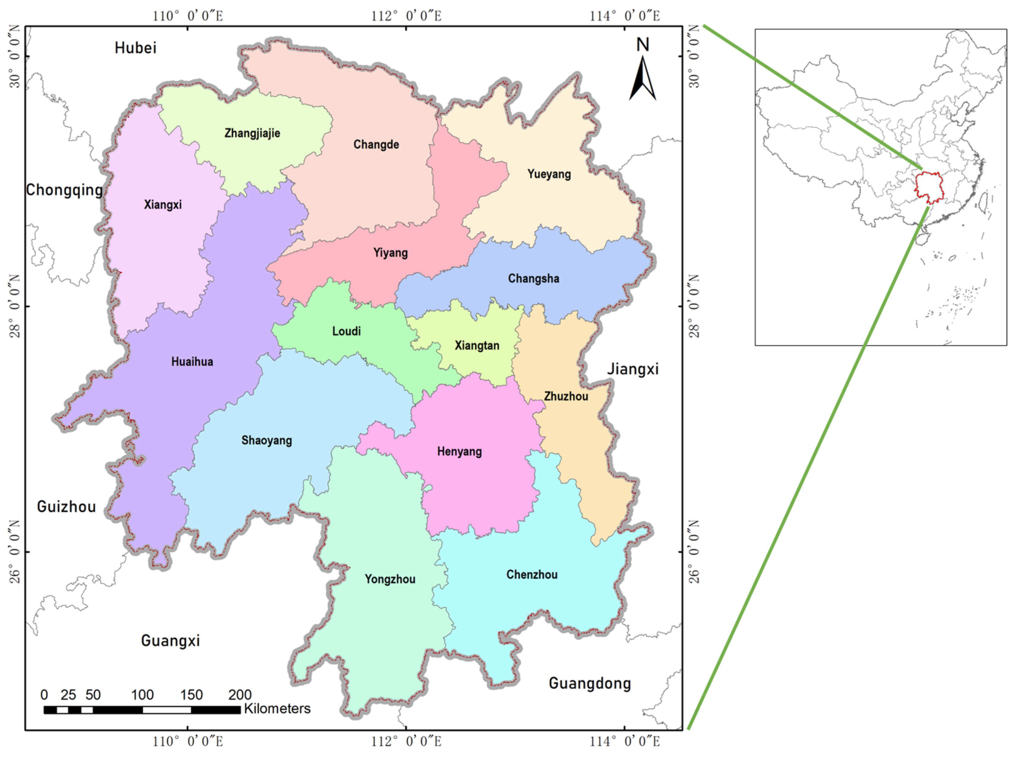
Figure 1. Study area: Hunan Province, China.
Forests 16 01632 g001
Figure 2. Spatial distribution of wildfire events and forest cover types in Hunan Province. (a) Wildfire occurrences from 2000 to 2024, with each red dot indicating one event; (b) Forest cover types across the province.
Forests 16 01632 g002
Figure 3. Explanatory variables for wildfire risk modeling (resampled to 1 km): (a) DEM; (b) slope; (c) aspect; (d) roads; (e) water; (f) railways; (g) NDVI; (h) GDP; (i) population density.
Forests 16 01632 g003
Figure 4. Workflow of data processing and model fitting.
Forests 16 01632 g004
Figure 5. Temporal patterns of wildfire occurrence in Hunan Province: (a) annual frequency; (b) monthly frequency; (c) ST-DBSCAN clustering results.
Forests 16 01632 g005
Figure 6. Spatial autocorrelation of wildfire probability: (a) probability distribution; (b) global Moran’s I; (c) LISA cluster map; (d) LISA p-value map. In the cluster map (c), red and blue areas denote statistically significant High–High clusters (hotspots) and Low–Low clusters (coldspots), respectively.
Forests 16 01632 g006
Figure 7. Predicted vs. observed wildfire probability for models. (a) KNN; (b) MLP; (c) SVR; (d) AdaBoost; (e) RF; (f) GWR; (g) GTWR; (h) GTWR-RFR. The x-axis represents the model-predicted wildfire occurrence probability, and the y-axis represents the actual wildfire occurrence probability. The red line denotes the fitted line.
Forests 16 01632 g007
Figure 8. Spatial patterns of local variable importance. (a) daily mean temperature; (b) 24 h precipitation; (c) daily mean wind speed; (d) DEM; (e) slope; (f) aspect; (g) canopy closure; (h) standing timber volume; (i) GDP; (j) population density; (k) distance from road; (l) distance from water. In the figure, red represents a positive impact, blue represents a negative impact, and yellow signifies a minimal impact. The color gradient from red to blue indicates a transition from positive to negative effects.
Forests 16 01632 g008
Figure 9. Spatial distribution of t-values for explanatory variables. (a) daily mean temperature; (b) 24 h precipitation; (c) daily mean wind speed; (d) DEM; (e) slope; (f) aspect; (g) canopy closure; (h) standing timber volume; (i) GDP; (j) population density; (k) distance from road; (l) distance from water.
Forests 16 01632 g009
Figure 10. Predicted wildfire probability and risk levels in Hunan Province for 2025 using the GTWR–RFR model. (a) Predicted wildfire probability; (b) wildfire risk classification, where green, blue, yellow, and red represent no, low, moderate, and high risk, respectively.
Forests 16 01632 g010
Figure 11. Monthly wildfire risk in Hunan Province for 2025. Panels (al) represent January to December, respectively. Wildfire risk increases from (a) January to (d) April, reaching its peak in April, decreases from (e) May to (h) August, and rises again from (i) September to (l) December.
Forests 16 01632 g011
Table 1. Data sources and spatial resolution of explanatory variables.
FactorsVariableSourceClassesSpatial
Resolution/
Units
Wildfire pointHistorical WildfiresNASA Fire Information Resource Management System (FIRMS)
https://firms.modaps.eosdis.nasa.gov/ (accessed on 21 October 2025)
Continuous
Meteorological factorsTemperature
Pressure
Humidity
Wind speed
Precipitation
Sunshine
High-resolution gridded datasets
https://crudata.uea.ac.uk/cru/data/hrg/ (accessed on 21 October 2025)
China Geospatial Data Cloud
http://data.cma.cn/ (accessed on 21 October 2025)
Continuous 0.1 °C
0.1 hPa
1%
0.1 m/s
0.1 mm
0.1 h
Terrain factorsDEM
Slope
Aspect
Geospatial Data Cloud
https://www.gscloud.cn/ (accessed on 21 October 2025)
Continuous1000 m
Vegetation factorsVegetation typeGeospatial Information Authority of Japan (GSI)
https://globalmaps.github.io/glcnmo.html (accessed on 21 October 2025)
Categorical 1000 m
NDVIMODIS Vegetation Index Products
https://modis.gsfc.nasa.gov/data/dataprod/mod13.php (accessed on 21 October 2025)
Categorical
Canopy closure
timber volume
National Smart Forest Resources Management Platform
https://www.stgz.org.cn/ldbggzpt/ (accessed on 21 October 2025)
Continuous
Anthropogenic factorsRoad
Water
Railway
Openstreetmap
https://www.openstreetmap.org/ (accessed on 21 October 2025)
Continuous1000 m
Socioeconomic factorsGDPResource and Environmental Science and Data Center,
https://www.resdc.cn/ (accessed on 21 October 2025)
Continuous1000 m
PopulationWorldPop
https://hub.worldpop.org/ (accessed on 21 October 2025)
Continuous
Table 2. VIF analysis for variable selection.
Model VariableVariable CodeVIFTOL
Canopy ClosureCC0.1715565.829003
Daily mean temperatureDMT0.1716995.824144
DEMDEM0.1736775.75782
Daily mean wind speedDMWS0.2033614.917362
SlopeSlope0.2118424.72051
AspectAspect0.259883.847925
Distance from waterNDW0.2697353.707344
24 h precipitationHP0.2879773.472499
Distance from roadNDR0.3142613.18207
Population densityPD0.3821882.616512
Standing timber volumeAVST0.3908552.558495
GDPGDP0.4208372.376215
Table 3. Model performance metrics (R2, RMSE, MAE, etc.).
KNNMLPSVRAdaBoostRFRGWRGTWRGTWR-RFR
R20.3760.5320.4780.6570.8020.8480.8850.969
Explained Variance Score0.2710.36970.33960.52090.57090.84810.88540.9696
Mean Absolute Error0.66470.60840.6190.54390.50350.26630.22550.1256
Mean Squared Error0.74570.64080.67050.490.43680.15210.11470.0304
Root Mean Squared Error0.86350.80050.81880.710.66090.38990.33870.1743
Explained sum of squares1061.91671.51249.61765.91813.714,640.215,486.215,661.7
Total sum of squares3813.53813.53813.53813.53813.818,78318,78318,783.0
Residual sum of squares2801.520,606.919,022.120,961.921,141.32856.12154.8570.8
Table 4. Global Moran’s I of residuals for all models.
ModelMoran’s IZ-Scorep-Value
AdaBoost0.6050213.28410
SVR0.6370224.57650
MLP0.5692200.68620
KNR0.6618233.31810
RFR0.5781203.83160
GWR0.3459121.95810
GTWR0.2959104.35450
GTWR-RFR0.246286.82030
Table 5. Descriptive statistics of GTWR-RFR coefficient estimates.
Model VariableCodeMeanSTDMinMedianMaxMoran’s Iz-Scorep-Value
Daily mean temperatureDMT0.0440.0280.0030.0380.5290.8002 282.2 0
24 h precipitationHP0.0460.0310.0030.040.5440.8471 298.880
Daily mean wind speedDMWS0.0560.0370.0030.0490.6820.8127 286.6 0
SlopeSlope0.0540.0320.0030.0480.3650.8525 300.6 0
AltitudeDEM0.1280.0970.0040.0970.7640.8454 298.10
AspectAspect0.0470.0270.0020.0430.4840.8598 303.30
Canopy ClosureCC0.0260.0210.0010.0220.510.8087 285.6 0
Standing timber volumeAVST0.0220.02100.0170.4450.8535 301.30
GDPGDP0.1520.11700.1170.7950.8382 295.50
Population densityPD0.1290.1030.0070.0950.8210.8685 306.20
Distance from roadNDR0.110.1050.0050.0780.850.8961 316.00
Distance from waterNDW0.140.1110.0060.1020.7840.8998 317.20
Table 6. Pixel count and percentage by wildfire risk category.
Risk
Classification
Fire
Probability
Pixels CountPercent (%)Recommended Measures
Non-fire risk<0.23,050,51345.01%negligible
Low-fire risk0.2~0.42,293,83433.85%routine prevention and monitoring
Moderate-fire risk0.4~0.6884,76913.06%proactive assessments
High-fire risk0.6>547,7888.08%Intensive monitoring and targeted prevention strategies
Disclaimer/Publisher’s Note: The statements, opinions and data contained in all publications are solely those of the individual author(s) and contributor(s) and not of MDPI and/or the editor(s). MDPI and/or the editor(s) disclaim responsibility for any injury to people or property resulting from any ideas, methods, instructions or products referred to in the content.