Abstract
The global forestry discourse frequently highlights the issue of ungulate browsing, which can significantly impact tree regeneration and tree species composition by inhibition of growth and elimination of certain, particularly ecologically valuable, tree species. The forestry field often utilizes the percentage of browsed trees within a specific area, ranging from single hunting grounds to broader provincial scales, as a metric of browsing intensity. This measure correlates with ungulate density, which is known to vary across landscapes, rendering spatially averaged browsing percentages less useful for silvicultural decisions even with accurate results. Addressing this gap, we utilized a GLMM with random effects to assess tree specific browsing pressure more appropriately. We incorporated data from two adjacent areas in the northeastern limestone Alps, focussing on the four important tree species in the region (Abies alba, Acer pseudoplatanus, Fagus sylvatica, and Picea abies). We analyzed data collected with distinct methodologies for the two regions, respectively, Austrian Federal Game Impact Monitoring and Austrian Regeneration and Browsing Monitoring of Federal Forests. Overall, the data documented browsing occurrence on 8933 trees over 632 sampling plots totalling 55,000 hectares. By comparing various models, including those with spatial considerations, we found that treating sampling plot location as a latent state variable improved the model fit and allowed prediction of browsing probability on a landscape scale. This study underlines the value of incorporating spatial elements into models for assessing browsing pressure and its spatial variations, thereby facilitating more informed silvicultural decisions.
1. Introduction
The interaction between wild ungulates and forest ecosystems, particularly in terms of tree browsing, presents significant challenges for forest management [1,2]. The imperative for enhancing tree species diversity is underpinned by the pressures of climate change, making it vital to favour tree species that are more resilient to rising temperatures [3]. These species, however, tend to be the preferred targets of ungulates, as evidenced by research conducted in countries like Germany, Switzerland, and Austria. Where browsing occurs on an intensive level, it can severely hinder forest regeneration [2,4,5]. Accurate detection of ungulate pressure across forest sites hinges on the establishment of systematic monitoring. Although regional monitoring systems, such as Federal Game Impact Monitoring (WEM) in Austria, exist, it is challenging for forest management to acquire precise and geographically detailed data. Browsing intensity is typically measured as the proportion of browsed tree shoots in given plots [2], limiting sampling to the species available within these plots.
Reimoser [1] advocated for a more nuanced assessment of browsing rates, noting the significant spatial and temporal variability driven by the movements of herbivores such as red deer, Cervus elaphus L. (Artiodactyla: Cervidae), chamois, Rupicapra rupicapra L. (Artiodactyla: Bovidae), and roe deer, Capreolus capreolus L. (Artiodactyla: Cervidae) due to, e.g., seasonal migrations and habitat preferences [6,7,8]. Johnson [9] categorized the spatial behaviours of animals into four levels, from their broad geographical distribution to specific resource selection behaviours that include dietary preferences. Factors such as tree species, silvicultural conditions, and game density variously impact these levels, from food selection to habitat preferences [10]. These behaviours directly influence tree regeneration, necessitating, we argue, a detailed analysis that distinguishes between these spatial levels.
Silviculture, the practice of managing tree species composition, is often thwarted by browsing herbivores, which can hinder or selectively inhibit the regeneration of certain tree species [11]. Browsing impacts are typically assessed by comparing actual conditions against a predefined standard, often using fenced plots for control [12]. However, discrepancies between browsing effects and silvicultural goals pose significant challenges. Moreover, the influence of game density on tree diversity is a critical concern [13]. While browsing rates are calculated for individual tree species and averaged at the chosen organizational level, significant spatial variations in game density suggest the need for spatial considerations in browsing analyses.
This leads to several pressing questions we confront in this study. First, how reliable are the observed browsing percentages, and how great is the magnitude of the confidence intervals? Second, with current methodologies, is it feasible to spatially map browsing probability? And third, is it feasible to spatially model the probability of browsing across the entire study area? By answering these research questions, we intend to provide management a tool that can support evidence-based silvicultural decision-making in the future.
2. Materials and Methods
2.1. Area Description
Our study leveraged data from two distinct regions within the northern Alps of Upper Austria (Figure 1), encompassing a combined total of 8933 trees across 632 plots in a 55,000-hectare area. The first study area, Wald-Wild Grünau Klaus (WWGK), is situated in the districts Gmunden and Kirchdorf (at 47.8° N, 14.0° E), 197 plots were recorded within this area. The second study area, the Nationalpark Kalkalpen (NPK), is located in the districts Kirchdorf and Steyr-Land (at 47.8° N, 14.4° E), 435 plots were recorded within this area. Both areas feature limestone bedrock and predominantly mixed forests where beech, Fagus sylvatica L. (Fagales: Fagaceae), fir, Abies sp. Mill. (Pinales: Pinaceae), spruce, Picea abies (L.) H. Karst (Pinales: Pinaceae), and sycamore, Acer pseudoplatanus L. (Sapindales: Sapindaceae) are common. The natural forest community at both study areas is a mixed spruce–fir–beech forest. Beech tends to dominate at lower elevations, whereas spruce becomes more dominant at higher elevations. However, due to anthropogenic influences, the proportion of spruce often exceeds what would be expected naturally. These areas experience an average temperature of 6 °C and receive roughly 1200 mm of precipitation annually. Elevation in the WWGK study area ranges from 550 to 2515 m above sea level (ASL), while in the NPK study area it spans from 385 to 1963 m ASL [14].
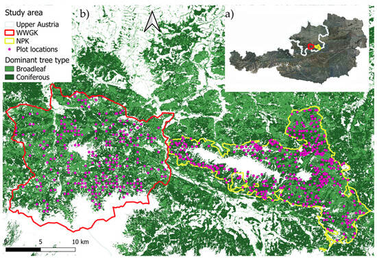
Figure 1.
Location of the study areas in Austria (a) with the dominant tree types [15] and plot locations (b).
Three large herbivore species are present in both study areas roe deer, C. capreolus, chamois, R. rupicapra, and red deer, C. elaphus. Roe deer and red deer are distributed throughout both study areas, while the occurrence of chamois is restricted to suitable habitats, typically characterized by steep slopes, rocky terrain or both.
2.2. Data Collection
We used data in the study area WWGK collected with the WEM methodology developed by the Austrian Research Centre for Forests (BFW). Following WEM, each sample plot covers 100 m2, corresponding to a circle with a radius of 5.64 m, and must include at least five saplings taller than 30 cm, each spaced at least 1.5 m apart. For every tree species present, data collection begins from the northern edge of the plot. At least 30 saplings over 30 cm in height are recorded for each species, with the requirement that a full eighth or sixteenth segment of the plot is always full inventoried. Additionally, up to 30 saplings per species with heights between 10 and 30 cm are documented. At each grid point, a selection of core plot characteristics is recorded, including coordinates, elevation, slope, and a brief description of site conditions. Ground vegetation and the dominant tree species in the overstory are also noted. For each sapling, the following information is gathered: tree species, height class, protection status (chemical, physical or no protection against browsing), evidence and timing of browsing of the leader shoot (distinguishing between current year, previous year, or both), and any signs of bark stripping. In cases where only part of the area is inventoried, the height class of the ten tallest saplings and the number of eighth-plot segments surveyed are also recorded. Modifications to this method led to the adoption of WEM-new, where only the five tallest trees of each species within a plot were assessed for browsing, as these are likely to become the future canopy [16,17]. Sample plots were assigned by superimposing a randomly positioned grid with 500 m spacing onto the study area. Only plots with less than 60% canopy cover were visited in the field. Sites lacking the potential for tree regeneration, such as meadows or dense old-growth stands, were pre-excluded from field sampling through GIS-based analysis. Data collection took place from August 2019 to September 2019 and from August 2020 to November 2020.
In the study area NPK, a different monitoring system developed by the Austrian Federal Forests (ÖBf), known as Regeneration and Browsing Monitoring of Federal Forests (JVSM), was utilized. This system involves 12.5 m2 (2 m radius) plots with at least three trees measuring between 10 and 300 cm in height. These plots are preferably located in clearings, and the spatial distribution is based on a random design. When clearings were not available, the plots were located in forest stands with regeneration. The data collection took place in two phases from June to July 2022 and from October to November 2022.
Browsing was defined consistently by both methods. Specifically, a plant was considered browsed if the leader shoot from the previous vegetation period and the following winter had been bitten off by wild ungulates. Browsing that occurred during the current vegetation period was excluded [16].
2.3. Binomial Confidence Interval Calculation
To estimate confidence intervals for proportions derived from binomial browsing data, we used the binconf function from the Hmisc package (version 5.2-2) [18] in R (version 4.5.0). This function provides accurate confidence intervals for binomial proportions using methods such as the Wilson score interval, which is preferred over the traditional normal approximation for proportions close to 0 or 1 or with small sample sizes. Given the discrete and bounded nature of the browsing data (i.e., browsed vs. unbrowsed), a binomial model was appropriate, and binconf allowed for robust and interpretable interval estimation aligned with the underlying data distribution.
2.4. Model Theory
It is well established that the probability of browsing on a tree sapling is influenced by several key factors, including tree species (i.e., composition and richness), the availability of alternative browse (i.e., other palatable plants), and the spatial distribution of ungulates [9,19,20]. Due to the lack of data on herbaceous plants, we assumed stem number per ha to be a reasonable proxy for the availability of alternative browse. If the distribution of ungulates across the landscape is heterogeneous, we would expect the spatial pattern of browsing probability to reflect this variation.
2.5. Model Specification
To analyze the proportion of browsed versus unbrowsed observations at each sample plot i, we specified a binomial mixed-effects model using the SpaMM (version 4.5.0) [21] package in R [22]. The response variable (browsing probability) was modelled as a binomial outcome, representing the number of browsed and unbrowsed observations, with a logit link function:
where p denotes the probability of browsing occurrence, and n represents the total number of observations (). The logit transformation was applied to model the relationship between the predictors and the browsing probability:
(Browsed, Unbrowsed) ~ Binomial(n, p),
logit(pi) = log(pi/1 − pi),
2.5.1. Fixed Effects
The fixed effects included treespecies and stemnumber as predictors:
where
ηj,i = β0 + β1j treespeciesj + β2 stemnumberi
- ηj,i is the prediction of the browsing probability depending on the treespecies j and the stemnumber i
- β0 is the intercept
- β1j and β2 are the estimated coefficients for the fixed effects
- treespeciesj is a categorical variable representing tree species
- stemnumberi is a continuous variable indicating the local density of young tree stems
2.5.2. Spatial Random Effects
We accounted for the unobserved spatial distribution of ungulates by modelling the spatial distribution of browsing pressure, i.e., autocorrelation, as a latent state. Namely, we included a spatial random effect using the Matérn covariance function. The spatial random effect u(s) was defined as a Gaussian process with mean zero and a Matérn covariance structure:
where
u(s) ~ GP (0, σ2 Mν(d))
- s = (x, y) represents the spatial coordinates of the observations,
- σ2 is the variance of the spatial effect,
- Mν(d) is the Matérn covariance function defined as:
Mν(d) = 1/(Г (ν) 2ν−1) × (κd)ν Κν (κd)
In this formulation:
- d denotes the Euclidian distance between observation locations,
- κ is a scale parameter, inversely related to the range of spatial correlation,
- ν is a smoothness parameter,
- Κν is the modified Bessel function of the second kind and order ν.
2.5.3. Final Model Specification
Combining fixed and random effects, the full model specification was:
where the spatial random effect u(xi, yi) follows a Gaussian process with Matérn covariance structure.
logit(pi) = β0 + β1 treespecies + β2 stemnumberi + u(xi, yi)
2.5.4. Estimation Procedure
The model parameters were estimated using the h-likelihood (hierarchical likelihood) approach implemented in the SpaMM package. This approach jointly estimates fixed effects, spatial random effects, and dispersion parameters by maximizing the penalized likelihood [21]. To determine the best model for explaining browsing probability, we followed a stepwise model selection procedure, progressively increasing model complexity and comparing models using the Akaike Information Criterion (AIC) [23]. For both study areas (WWGK and NPK separately), we began with a simple model including only tree species as a predictor. We then added stem_number as an additional covariate and finally included a spatial random effect using a Matérn covariance structure (Matern(1|x + y)) to account for the unobserved distribution of ungulates.
3. Results
3.1. Browsing Percentage Analysis
Regarding the reliability of the observed browsing percentages and the magnitude of the confidence intervals, our analysis of the original dataset revealed distinct browsing percentages across the four tree species and the two study areas (Figure 2). In the study area WWGK, sycamore and fir both exhibited the highest browsing probabilities at 33%, with spruce at the lower end at 8%, and beech in the middle at 20%. The NPK study area presented higher browsing rates overall; sycamore reached 45%, fir remained at 33%, beech increased to 27%, and spruce to 12%. The larger sample size in NPK resulted in narrower confidence intervals. Notably, fir consistently showed the broadest confidence intervals across both areas, indicating the smallest sample size on this species.
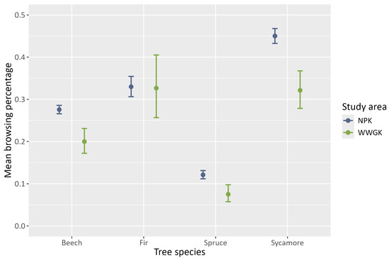
Figure 2.
Mean observed browsing percentage with 95% confidence intervals per tree species.
We observed clear spatial variation in browsing percentages per plot for each tree species (Figure 3). The spatial patterns differ between tree species; however, they share a common hotspot located in the centre of NPK. It is important to note that fir was recorded at significantly fewer plots compared to the other species.
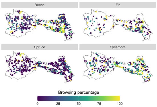
Figure 3.
Spatial distribution of browsing percentage per sample plot divided into tree species.
3.2. Model Comparisons and Predictions
For each study area, model performance improved as additional predictors were included, as indicated by decreasing AIC values (Table 1). The most complex model—including tree species, stem density, and the spatial random effect—had the lowest AIC and was therefore selected for further analysis. This stepwise approach reflects our assumption that browsing probability is influenced not only by species identity and local stem density, but also by spatial processes operating above plot scale.

Table 1.
Comparison of AIC values.
In both study areas, spruce was the tree species least likely to be browsed while sycamore was most likely to be browsed. Further, as browse availability increased (i.e., stem number) browsing probability went down. Nu, the smoothing coefficient, was higher in WWGK (Table 2) than NPK (Table 3). In other words, spatial correlations in browsing probability between locations decayed more quickly with increasing separation distance in WWGK than in NPK.
Table 2.
Statistical parameters of the final model of study area WWGK.
Table 3.
Statistical parameters of the final model of study area NPK.
Comparing the prediction of the three models for each study area, we found browsing probabilities for all tree species decreased with increasing stem numbers (Figure 4). For the spatial model predictions, we assumed a randomly located point within the study area. Interestingly, incorporating the spatial random effect into the model results in lower predicted browsing probabilities compared to models that include only tree species and stem number as fixed effects.
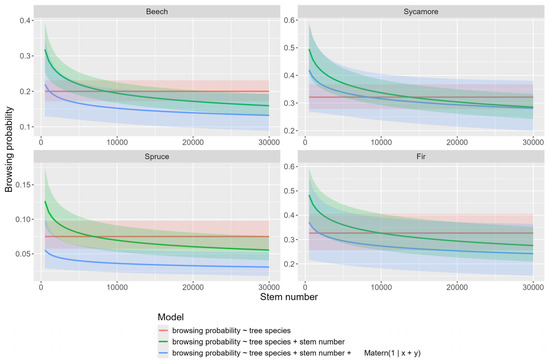
Figure 4.
Comparison of WWGK models for each tree species.
We predicted the spatial distribution of browsing probabilities in WWGK and NPK for beech, thereby showing the variability in unobserved drivers of browsing intensity, i.e., ungulate distribution (Figure 5). Spatial predictions, showcased in Figure 5 for study area WWGK and study area NPK, respectively, affirm the capability of our spatial model to forecast browsing probabilities across all tree species. Our results indicate that interspecific browsing patterns within a plot may allow for predicting the browsing likelihood of tree species that are not locally present but occur elsewhere in the study area. The figures show spatial pattens with low to high browsing probability across all tree species (Appendix B).
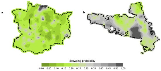
Figure 5.
Spatial prediction of browsing probability of beech at medium stem numbers for (a) WWGK (6803 stems per ha) and (b) NPK (9552 stems per ha).
4. Discussion and Conclusions
Modelling browsing probability spatially allows the likelihood of a tree species being browsed to be predicted for the entire area, even if it was not recorded in every plot. This insight is essential for silvicultural planning, as it facilitates the integration of wildlife impact—distinct from damage—into the strategic framework of forest management. Our study underscores the significant advantages of spatially explicit browsing analyses for practical silviculture applications. With respect to our first research question—how reliable the observed browsing percentages are—we found that percentages can be highly stable when based on sufficiently large sample sizes. Confidence intervals were narrow when >200 stems were recorded (see Figure A10), demonstrating that browsing percentages provide reliable information under these conditions. This shows that the data quality is not inherently weak but strongly dependent on sample size. However, even when aggregated browsing observations are statistically robust, indicated by narrow confidence intervals, a single browsing percentage lacks spatial resolution and does not capture local variability at the stand level. Thus, while browsing percentages are reliable for broad-scale monitoring, they are not sufficient to describe fine-scale heterogeneity.
Turning to our second research question—whether it is feasible to spatially map browsing probability at the plot level—the findings suggest that plot-wise mapping provides some spatial detail but is of limited use for management. This limitation stems from the small sample sizes at many plots and the dependence of results on the local tree species composition. For instance, in WWGK, plots with fewer than 20 stems showed strongly fluctuating browsing percentages, underlining the uncertainty of this approach. Therefore, while technically feasible, plot-level mapping cannot yet provide robust information for decision-making.
Our third research question asked whether it is feasible to spatially model browsing probability across the entire study area. Here, our results clearly demonstrate that this is possible. By applying spatial modelling to commonly collected field data, we were able to extrapolate browsing probability to unsampled locations, revealing gradients of browsing pressure across the landscape. This modelling step added explanatory power beyond browsing percentages and plot-level mapping, and it highlighted browsing hotspots that would otherwise remain undetected. This approach allows for extrapolation to unsampled locations, thereby improving the ability to detect and interpret spatial patterns of browsing pressure across the landscape.
We observed a clear trend where increased stem numbers corresponded with lower browsing probabilities, revealing distinct patterns of increased browsing probability across different locations. This finding directly supports the model results for question three, showing that stem density serves as a meaningful predictor for browsing probability and likely acts as a proxy for forage availability. Browsing probability depends on numerous factors. For example, different studies show that for the individual tree browsing probability depends on which plants are growing in the neighbourhood and the distance to the neighbouring plants [19,24,25,26]. Alternative browsing opportunities are not limited to trees but also include non-tree palatable vegetation. As such, the height, quality and density of the surrounding non-tree vegetation can impact tree browsing [27]. These predictors were not recorded in our study. We assume that in most cases stem number is a good proxy for the availability of overall palatable plants.
The study by Borowski et al. [19] highlighted the influence of game density and tree species diversity on browsing, concepts our model encapsulated as a latent variable. Incorporating game density explicitly could enhance model accuracy but at the cost of data collection efficiency. Game density is not uniformly distributed in time nor in space [6,7,8]. Even in periods with low game densities, local accumulations of herbivores can result in locally high browsing rates. The process of browsing is affected less by average game density than by usage of a certain area for food consumption [28]. Tree species composition within a plot is an important factor influencing browsing probability. At the plot level, a higher number of tree species was associated with a lower probability of individual trees being browsed. In contrast, at a broader spatial scale (i.e., between plots), higher tree species richness was associated with an increased overall browsing probability [29]. Such factors make modelling browsing data spatially challenging due to the different hierarchical levels of the same process. So, treating game density as a latent variable is an option to include this spatial component and thereby explain the most important driver of browsing occurrence. The observed spatial distribution appears to reflect the general distribution of ungulates in the study area, as suggested by the authors’ field experience. However, we would caution against a direct translation of browsing pressure patterns into ungulate densities for several reasons. First, browsing intensity represents cumulative exposure over the course of an entire year. We assume that all three ungulate species exhibit considerable migratory movements, and browsing intensity is likely to vary seasonally. Second, little is currently known about the species-specific browsing preferences of the different ungulate species. Thus, the resulting browsing pressure distribution is best understood as the combined outcome of the spatial and temporal occurrence of multiple species together with their shifting preferences for different tree species over time. At present, we see limited opportunities to disentangle these factors. Nevertheless, our approach—by allowing for the representation of varying browsing probabilities—constitutes an important step toward linking browsing pressure with ungulate densities. Future research should therefore build upon our positive findings for question three by integrating spatial browsing data with independent measures of ungulate occurrence (e.g., pellet counts, camera traps) in order to validate and refine these models.
The definition of browsing, particularly the significance of browsing on leading tree shoots, presents a challenge in comparing studies, necessitating clear definitions for accurate comparisons [1]. The two monitoring systems employed in our study, WEM and JVSM, differ substantially in their design. WEM uses larger plots and thus captures a wider range of regeneration and rarer tree species, while JVSM uses smaller but more numerous plots, providing denser spatial coverage. These methodological differences inevitably influence the model results.
For our models, WEM data proved valuable in representing rare tree species and capturing browsing patterns across broader gradients, but the lower plot density reduced its ability to reflect local variation in browsing pressure. In contrast, JVSM data, with its higher spatial resolution, yielded more reliable estimates at the stand level but was less informative for species that occur infrequently. This difference matters for model interpretation: WEM-based results are well suited for regional-scale analyses and long-term trend detection, whereas JVSM-based results provide stronger support for operational silvicultural decisions at the stand or management-unit level.
From a practical perspective, this means that the choice of monitoring system should depend on the management question at hand. If the aim is to identify broad-scale patterns of browsing risk, WEM offers advantages despite its coarser spatial resolution. If the goal is to guide site-level interventions, JVSM delivers more precise and actionable information. Our spatial modelling approach partly compensates for the weaknesses of each system by incorporating latent spatial structure and interspecific browsing information, thereby enhancing robustness regardless of the monitoring design. However, the comparison also highlights that the confidence and applicability of spatial browsing models are directly tied to the underlying monitoring data.
Overall, the results underscore that WEM and JVSM are not interchangeable but complementary. WEM is better suited to policy-oriented monitoring at regional scales, while JVSM provides more reliable inputs for practical forest management. Recognizing these strengths and limitations is crucial for interpreting model outputs and for designing future monitoring strategies.
The random effects coefficients of the final models show that there is a difference between the study areas. It is clear, a priori, that there must be a difference, because different methods were applied to collect the data with a different spatial contextualization of the forest structure. But the values also showed that the browsing probabilities in WWGK varied more and with greater amplitude in close proximities than in NPK. Probably this was due to the influence of varying deer densities over time and space in the different study areas. This provides further evidence in support of research question three, namely that spatial modelling can reveal meaningful differences between study areas which are not visible in browsing percentages alone. These conditions need to be investigated in further research. The random effect reflecting ungulate distribution in our study is influenced by a range of ecological and anthropogenic factors. While habitat availability plays an important role, spatial patterns of ungulate occurrence are also affected by recreational activity, hunting pressure, forest management regimes and predation [30,31,32,33]. These factors may not only act independently but also interact with each other, potentially leading to overlapping or compounding effects on ungulate distribution [34]. Introducing a spatial component into browsing analysis offers novel insights for forestry management, particularly in identifying areas under significant browsing pressure, crucial for informed silvicultural decision-making. The temporal and species-specific browsing patterns, such as the late winter preference for fir and summer browsing of sycamore, provide valuable guidance for wildlife management and the introduction of new tree species [35,36]. The challenge ahead lies in developing and refining methods for more accurate browsing analysis. Alternatives like the k-Tree method offers improved browsing estimates but may fall short in capturing essential data like stem numbers, crucial for models like ours [37]. Employing transects for browsing surveys could yield the sample sizes necessary for robust probability assessments.
Applying a spatial modelling approach to browsing data provides a more realistic assessment of game impact on tree regeneration than relying solely on conventional browsing percentages. To address the limitations posed by small sample sizes and high uncertainty, it is essential to implement methods that allow for more efficient recording of a larger number of trees across the entire study area and not only limited to fixed plots.
Author Contributions
T.B.: Writing—review & editing, Formal analysis, Writing—original draft, Methodology, Visualization, Investigation, Conceptualization. D.D.: Writing—review & editing, Formal analysis, Methodology, Visualization, Data curation, Conceptualization. K.W.-D.: Writing—review. E.H.: Conceptualization, Data curation. All authors have read and agreed to the published version of the manuscript.
Funding
This research received no external funding.
Data Availability Statement
Restrictions apply to the availability of these data. Data were obtained from the Austrian Federal Forests as well as the Government of Upper Austria and are available from the corresponding author with the permission of the named institutions.
Acknowledgments
We are grateful to the Austrian Federal Forests and the Department of Agriculture and Forestry of the Government of Upper Austria who provided the data for this study.
Conflicts of Interest
The authors declare no conflicts of interest.
Abbreviations
The following abbreviations are used in this manuscript:
| BFW | Austrian Research Centre for Forests |
| JVSM | Regeneration and Browsing Monitoring of Federal Forests |
| NPK | National Park Kalkalpen |
| ÖBf | Austrian Federal Forests |
| WEM | wildlife impact monitoring |
| WWGK | forest and wildlife management project Grünau Klaus |
Appendix A
The distribution of stem numbers, an essential factor in our analysis, is depicted in Figure A1. In the study area WWGK there was significant variability in stem numbers, even within small geographical scales, particularly noticeable in the southeastern region. In contrast, in the study area NPK there was a more uniform stem number distribution. The application of different data collection methodologies in WWGK led to some plots lacking stem number data, which necessitated the use of median stem numbers for model development in these instances.

Figure A1.
Total stem number per ha for each plot with the outlines of the two study areas in grey.
Appendix B

Figure A2.
Prediction of spatial browsing probability for spruce in the NPK study area, divided into low (5572 = 25% quantile), medium (9552 = median) and high (19,697.5 = 75% quantile) stem number in total.
Figure A3 and Figure A4 show the model predictions for each tree species at study area NPK. The model calculated the browsing probability for three different stem numbers.

Figure A3.
Prediction of spatial browsing probability for beech in the NPK study area, divided into low (5572 = 25% quantile), medium (9552 = median) and high (19,697.5 = 75% quantile) stem number in total.

Figure A4.
Prediction of spatial browsing probability for fir in the NPK study area divided into low (5572 = 25% quantile), medium (9552 = median) and high (19,697.5 = 75% quantile) stem number in total.

Figure A5.
Prediction of spatial browsing probability for sycamore in the NPK study area divided into low (5572 = 25% quantile), medium (9552 = median) and high (19,697.5 = 75% quantile) stem number in total.
Figure A6, Figure A7, Figure A8 and Figure A9 show the prediction of the model for each tree species at study area WWGK. The model calculated the browsing probability for three different stem numbers.

Figure A6.
Prediction of spatial browsing probability for spruce in the WWGK study area divided into low (2501 = 25% quantile), medium (6803 = median) and high (27,098.75 = 75% quantile) stem number in total.

Figure A7.
Prediction of spatial browsing probability for beech in the WWGK study area divided into low (2501 = 25% quantile), medium (6803 = median) and high (27,098.75 = 75% quantile) stem number in total.

Figure A8.
Prediction of spatial browsing probability for fir in the WWGK study area, divided into low (2501 = 25% quantile), medium (6803 = median) and high (27,098.75 = 75% quantile) stem number in total.

Figure A9.
Prediction of spatial browsing probability for sycamore in the WWGK study area divided into low (2501 = 25% quantile), medium (6803 = median) and high (27,098.75 = 75% quantile) stem number in total.
Appendix C
The figure below (Figure A10) illustrates the expected confidence level as a function of the number of inspected trees, depending on the browsing probability. Owing to the binomial nature of browsing data, uncertainty is dependent on the underlying browsing proportion. For instance, if the expected browsing level is 50%, a sample size of approximately 400 trees is required to achieve a confidence interval of 10% (±5%).

Figure A10.
Estimation uncertainty depending on sample size and browsing probability.
References
- Reimoser, F. Hinweise Zum Richtigen Gebrauch von Verbisskennzahlen. Schweiz. Z. Für Forstwes. 1999, 150, 184–186. [Google Scholar] [CrossRef][Green Version]
- Bödeker, K.; Ammer, C.; Knoke, T.; Heurich, M. Determining Statistically Robust Changes in Ungulate Browsing Pressure as a Basis for Adaptive Wildlife Management. Forests 2021, 12, 1030. [Google Scholar] [CrossRef]
- Ruhm, W. Waldbauliche Möglichkeiten in Zeiten Des Klimawandels. BFW-Praxisinformation 44 Wege Zum Klimafitten Wald 2017, 44, 14–18. [Google Scholar]
- Kupferschmid, A.D.; Brang, P.; Bugmann, H. Assessment of the Impact of Ungulate Browsing on Tree Regeneration. Schweiz. Z. Fur Forstwes. 2019, 170, 125–134. [Google Scholar] [CrossRef]
- Nopp-Mayr, U.; Reimoser, S.; Reimoser, F.; Sachser, F.; Obermair, L.; Gratzer, G. Analyzing Long-Term Impacts of Ungulate Herbivory on Forest-Recruitment Dynamics at Community and Species Level Contrasting Tree Densities versus Maximum Heights. Sci. Rep. 2020, 10, 20274. [Google Scholar] [CrossRef] [PubMed]
- Krofel, M.; Luštrik, R.; Stergar, M.; Jerina, K. Habitat Use of Alpine Chamois (Rupicapra Rupicapra) in Triglav National Park. In Climaparks—Climate Change and Management of Protected Areas; Ljubljana, Slovenia, 2013; pp. 1–13. Available online: https://www.researchgate.net/publication/297689519_Habitat_use_of_Alpine_chamois_Rupicapra_rupicapra_in_Triglav_National_Park (accessed on 24 September 2025).
- Schwegmann, S.; Hendel, A.L.; Frey, J.; Bhardwaj, M.; Storch, I. Forage, Forest Structure or Landscape: What Drives Roe Deer Habitat Use in a Fragmented Multiple-Use Forest Ecosystem? For. Ecol. Manag. 2023, 532, 120830. [Google Scholar] [CrossRef]
- Luccarini, S.; Mauri, L.; Ciuti, S.; Lamberti, P.; Apollonio, M. Red Deer (Cervus Elaphus) Spatial Use in the Italian Alps: Home Range Patterns, Seasonal Migrations, and Effects of Snow and Winter Feeding. Ethol. Ecol. Evol. 2006, 18, 127–145. [Google Scholar] [CrossRef]
- Johnson, D.H. The Comparison of Usage and Availability Measurements for Evaluating Resourece Preference. Ecology 1980, 61, 65–71. [Google Scholar] [CrossRef]
- Borowik, T.; Cornulier, T.; Jędrzejewska, B. Environmental Factors Shaping Ungulate Abundances in Poland. Acta. Theriol. 2013, 58, 403–413. [Google Scholar] [CrossRef]
- Kupferschmid, A.D.; Heiri, C.; Huber, M.; Fehr, M.; Frei, M.; Gmür, P.; Imesch, N.; Zinggeler, J.; Brang, P.; Clivaz, J.C.; et al. Einfluss Wildlebender Huftiere Auf Die Waldverjüngung: Ein Überblick Für Die Schweiz. Schweiz. Z. Fur Forstwes. 2015, 166, 420–431. [Google Scholar] [CrossRef]
- Reimoser, F.; Odermatt, O.; Roth, R.; Suchant, R. Die Beurteilung von Wildverbiss Durch SOLL-IST-Vergleich. Allg. Forst Und Jagdztg. 1997, 168, 214–227. [Google Scholar]
- Kuiters, A.T.; Slim, P.A. Regeneration of Mixed Deciduous Forest in a Dutch Forest-Heathland, Following a Reduction of Ungulate Densities. Biol. Conserv. 2002, 105, 65–74. [Google Scholar] [CrossRef]
- Kilian, W.; Müller, F.; Starlinger, F. Die Forstlichen Wuchsgebiete Österreichs: Eine Naturraumgliederung Nach Waldökologischen Gesichtspunkten; Forstliche Bundesversuchsanstalt: Wien, Austria, 1993. [Google Scholar]
- European Union’s Copernicus Land Monitoring Service information. Dominant Leaf Type 2021 (Raster 10 m), Europe, Yearly. Available online: https://land.copernicus.eu/en/products/high-resolution-layer-forests-and-tree-cover/dominant-leaf-type-2021-raster-10-m-europe-yearly (accessed on 16 July 2025).
- Schodterer, H. Bundesweites Wildeinflussmonitoring (WEM). Forstschutz Aktuell 2006, 36, 7–12. [Google Scholar]
- Schodterer, H. Bundesweites Wildeinflussmonitoring—2018; Praxisinformation 48; Bundesforschungszentrum für Wald: Wien, Austria, 2019. [Google Scholar]
- Harrell, F.E., Jr. Hmisc: Harrell Miscellaneous. Available online: https://cran.r-project.org/web/packages/Hmisc/Hmisc.pdf (accessed on 15 April 2025).
- Borowski, Z.; Gil, W.; Bartoń, K.; Zajączkowski, G.; Łukaszewicz, J.; Tittenbrun, A.; Radliński, B. Density-Related Effect of Red Deer Browsing on Palatable and Unpalatable Tree Species and Forest Regeneration Dynamics. For. Ecol. Manag. 2021, 496. [Google Scholar] [CrossRef]
- Milligan, H.T.; Koricheva, J. Effects of Tree Species Richness and Composition on Moose Winter Browsing Damage and Foraging Selectivity: An Experimental Study. J. Anim. Ecol. 2013, 82, 739–748. [Google Scholar] [CrossRef]
- Rousset, F.; Ferdy, J.-B. Testing Environmental and Genetic Effects in the Presence of Spatial Autocorrelation. Ecography 2014, 37, 781–790. [Google Scholar] [CrossRef]
- R Core Team. R: A Language and Environment for Statistical Computing; R Foundation for Statistical Computing: Vienna, Austria, 2021. [Google Scholar]
- Akaike, H. A New Look at the Statistical Model Identification. IEEE Trans. Automat. Contr. 1974, 19, 716–723. [Google Scholar] [CrossRef]
- Holík, J.; Janík, D.; Hort, L.; Adam, D. Neighbourhood Effects Modify Deer Herbivory on Tree Seedlings. Eur. J. For. Res. 2021, 140, 403–417. [Google Scholar] [CrossRef]
- Champagne, E.; Tremblay, J.P.; Côté, S.D. Spatial Extent of Neighboring Plants Influences the Strength of Associational Effects on Mammal Herbivory. Ecosphere 2016, 7, e01371. [Google Scholar] [CrossRef]
- Brault, B.; Tremblay, J.P.; Thiffault, N.; Royo, A.A.; Côté, S.D. Successful Forest Restoration Using Plantation at High Deer Density: How Neighboring Vegetation Drives Browsing Pressure and Tree Growth. For. Ecol. Manag. 2023, 549, 121458. [Google Scholar] [CrossRef]
- Pietrzykowski, E.; McArthur, C.; Fitzgerald, H.; Goodwin, A.N. Influence of Patch Characteristics on Browsing of Tree Seedlings by Mammalian Herbivores. J. Appl. Ecol. 2003, 40, 458–469. [Google Scholar] [CrossRef]
- Donini, V.; Corlatti, L.; Ferretti, F.; Carmignola, G.; Pedrotti, L. Browsing Intensity as an Index of Ungulate Density across Multiple Spatial Scales. Ecol. Indic. 2024, 163, 112131. [Google Scholar] [CrossRef]
- Ohse, B.; Seele, C.; Holzwarth, F.; Wirth, C. Different Facets of Tree Sapling Diversity Influence Browsing Intensity by Deer Dependent on Spatial Scale. Ecol. Evol. 2017, 7, 6779–6789. [Google Scholar] [CrossRef]
- Marion, S.; Santos, G.C.; Herdman, E.; Hubbs, A.; Kearney, S.P.; Cole Burton, A. Mammal Responses to Human Recreation Depend on Landscape Context. PLoS ONE 2024, 19, e0300870. [Google Scholar] [CrossRef]
- Griesberger, P.; Kunz, F.; Reimoser, F.; Hackländer, K.; Obermair, L. Spatial Distribution of Hunting and Its Potential Effect on Browsing Impact of Roe Deer (Capreolus Capreolus) on Forest Vegetation. Diversity 2023, 15, 613. [Google Scholar] [CrossRef]
- Kramer, K.; Groot Bruinderink, G.W.T.A.; Prins, H.H.T. Spatial Interactions between Ungulate Herbivory and Forest Management. For. Ecol. Manag. 2006, 226, 238–247. [Google Scholar] [CrossRef]
- Heurich, M.; Brand, T.T.G.; Kaandorp, M.Y.; Šustr, P.; Müller, J.; Reineking, B. Country, Cover or Protection: What Shapes the Distribution of Red Deer and Roe Deer in the Bohemian Forest Ecosystem? PLoS ONE 2015, 10, e0120960. [Google Scholar] [CrossRef] [PubMed]
- Ausilio, G.; Wikenros, C.; Sand, H.; Devineau, O.; Wabakken, P.; Eriksen, A.; Aronsson, M.; Persson, J.; Mathisen, K.M.; Zimmermann, B. Contrasting Risk Patterns from Human Hunters and a Large Carnivore Influence the Habitat Selection of Shared Prey. Oecologia 2025, 207, 118. [Google Scholar] [CrossRef]
- Odermatt, O. Wildverbiss: Wann Sind Die Kritischen Phasen? Available online: https://www.waldwissen.net/de/waldwirtschaft/schadensmanagement/wildschaeden/wildverbiss-kritische-phasen (accessed on 14 August 2023).
- Häsler, H.; Senn, J. Ungulate Browsing on European Silver Fir Abies Alba: The Role of Occasions, Food Shortage and Diet Preferences. Wildl. Biol. 2012, 18, 67–74. [Google Scholar] [CrossRef]
- Kupferschmid, A.D. Monitoring des Wildeinflusses: Wichtige Merkmale und Beispiel einer Stichprobeninventur. Available online: https://www.google.com/url?sa=t&source=web&rct=j&opi=89978449&url=https://www.forstverein.ch/download/pictures/5f/zjzw33ukk1ogdaty3f3n4y0y6vue6y/01_kupferschmid_sfv_wald_wild_kurs_2020.pdf&ved=2ahUKEwjk2I3DtvaPAxWi1AIHHcuvC5wQFnoECCQQAQ&usg=AOvVaw28sJHgxiMq9EFbpp1rypYk (accessed on 5 January 2025).
Disclaimer/Publisher’s Note: The statements, opinions and data contained in all publications are solely those of the individual author(s) and contributor(s) and not of MDPI and/or the editor(s). MDPI and/or the editor(s) disclaim responsibility for any injury to people or property resulting from any ideas, methods, instructions or products referred to in the content. |
© 2025 by the authors. Licensee MDPI, Basel, Switzerland. This article is an open access article distributed under the terms and conditions of the Creative Commons Attribution (CC BY) license (https://creativecommons.org/licenses/by/4.0/).