Abstract
The cooling effect of urban forests has been widely investigated to support climate-adaptive spatial planning. However, studies on the impacts of key landscape drivers have often produced conflicting results, limiting their practical applicability. These inconsistencies may stem from an oversimplified focus on the global effects of individual factors, while neglecting non-linear threshold behaviors and pairwise interactions. To address this gap, this study employed an interpretable machine learning framework (XGBoost-SHAP) to quantify the seasonal non-linearities, thresholds, and interaction effects of landscape drivers on urban forest cooling in Suzhou, a subtropical Chinese city. The results indicate that the combined explanatory power of neighboring water body proportion (NWP), neighboring green space proportion (NGP), vegetation density (NDVI), spatial characteristics (Area, SHAPE), and elevation on the cooling intensity of urban forest patches was strongest in summer (R2 = 0.615) and weakest in winter (R2 = 0.316). Among these, NWP, NGP, and NDVI were the dominant drivers, while patch area and shape exhibited weaker marginal effects. NWP significantly enhances cooling only after exceeding seasonal critical thresholds (11%–15%). NGP contributed positively above ~40% in warm seasons but suppressed cooling above 37% in winter. Patch area exhibits a logarithmic relationship with cooling intensity, with a critical threshold of approximately 2.48 ha and saturation thresholds between 12 and 14 ha. SHAPE exerted positive effects in spring and winter, negative effects in summer, and a transition from negative to positive in autumn. Notably, significant, threshold-modulated interactions were identified, including those between NDVI and NWP, SHAPE and NDVI, SHAPE and NGP, NWP and NDVI, NWP and NGP, and NGP and NDVI. In each interaction, the first factor regulates and reverses the effect of the second once specific thresholds are exceeded. This study provides actionable, evidence-based guidance for the planning and optimized design of urban forests.
1. Introduction
Rapid urbanization has profoundly altered the natural landscape and energy balance of the earth’s surface, exacerbating the urban heat island (UHI) effect [1,2,3]. The UHI effect not only directly endangers human health [4,5] but also intensifies multiple crises related to energy, environment, and ecology, significantly impacting urban sustainable development and residents’ quality of life [6,7]. IPCC assessment reports emphasize that global warming is increasing the frequency, intensity, and duration of extreme heat events [8]. Against this backdrop, identifying and promptly implementing effective UHI mitigation strategies is urgently needed. Urban green spaces are widely recognized as a cost-effective and critical nature-based solution (NbS) to address various challenges posed by urbanization, particularly in mitigating the UHI effect [9,10]. The cooling effect of urban green spaces is primarily achieved through transpiration and shading effect, supplemented by modifications to surface properties [11,12]. Therefore, understanding the landscape factors and driving mechanisms that control the intensity of its cooling effect is crucial for proposing specific and feasible landscape planning strategies.
Numerous studies have demonstrated that the cooling effect of green spaces is influenced by factors such as their size, spatial geometry, surrounding landscape composition, and local climatic conditions [13,14,15,16]. It is noteworthy that inconsistent findings have been observed across existing research. For instance, there is significant divergence in the literature regarding the impact of patch shape on the cooling effect of green space. Some studies suggest that geometrically regular and compact green spaces exhibit better cooling performance than irregular ones [13,17,18], while others argue the opposite [19,20,21]. Still, other researchers contend that shape has a negligible influence on the cooling effect of green spaces [22]. Contrary to conventional understanding, Zhou et al. have found that the area and Normalized Difference Vegetation Index (NDVI) of green space patches are not reliable predictors of their cooling effect in all cases, as their influence is modulated by the surrounding landscape composition [22]. These inconsistencies severely limit the practical application of the findings. A likely reason for these inconsistencies lies in the complex interactions between the landscape factors of green spaces and their cooling effects, which linear models fail to adequately capture.
Recent studies have confirmed that the cooling effects of spatially adjacent green spaces and water bodies on the thermal environment are not independent; rather, they interact in a mutually reinforcing manner [23,24]. Therefore, quantifying the impact of adjacent water bodies on the cooling effect of green space patches is crucial. Previous studies have widely employed multiple linear regression models to analyze the landscape drivers of the cooling effect of green spaces [13,25,26]. Such models are effective in identifying linear relationships among variables, determining the relative importance and direction of influence of various factors, and quantifying the joint effects of multiple drivers. However, this approach struggles to capture potential non-linear relationships, threshold effects, and interaction effects between variables. Neglecting the threshold and interaction effects between influencing factors of the cooling effect may lead to biased assessments (underestimation or overestimation) of individual factor contributions and oversight of critical relationships (e.g., the shape of green spaces playing a more significant role in the cooling effect at certain size thresholds). Consequently, such omissions can result in divergent or misleading conclusions compared to a more comprehensive analysis that accounts for these interactions. To overcome the limitations of traditional linear regression in capturing non-linear relationships and interaction effects, this study employs the extreme gradient boosting (XGBoost) machine learning model. This model effectively identifies complex non-linear thresholds and interactive effects influencing the cooling impact of green spaces, while providing reliable feature importance evaluation, thereby more accurately revealing the underlying mechanisms [27].
To address this gap, this study takes Suzhou, a subtropical city rich in blue-green infrastructure, as a case study. By employing the XGBoost model combined with SHapley Additive exPlanations (SHAP) interpretation methods, it aims to: (1) quantify the seasonal variations in the effects of landscape drivers on the cooling intensity of forest patches; (2) reveal the non-linear driving mechanisms and threshold effects of landscape factors on the cooling intensity of forest patches; and (3) identify pairwise interactions and interaction thresholds among landscape drivers. Based on the findings, the study further proposes threshold-informed optimization strategies for urban forest planning.
2. Methodology
2.1. Study Area
The study area is located in Suzhou, Jiangsu Province (longitude 119°55′–121°20′ E, latitude 30°47′–32°02′ N), in eastern China (Figure 1a). Suzhou borders Shanghai to the east, Zhejiang Province to the south, Taihu Lake to the west, and the Yangtze River to the north (Figure 1b). Administratively, Suzhou consists of six urban districts and four county-level cities, with a total area of approximately 8657.3 km2, of which rivers, lakes, and wetlands account for 34.6%. By the end of 2023, the permanent population reached 12.96 million [28]. Climatically, Suzhou experiences a northern subtropical monsoon climate, characterized by four distinct seasons—hot and humid summers and cold, damp winters. In 2023, the average annual temperature in the urban area was 18.5 °C, and the average annual precipitation was approximately 1414.2 mm, with the majority concentrated in the summer [29]. This study focuses on the urban core of Suzhou, which includes the Gusu, Xiangcheng, and Huqiu Districts, as well as the Suzhou Industrial Park, covering a total area of about 2035 km2. This study specifically focuses on the urban forests within this delineated urban core.
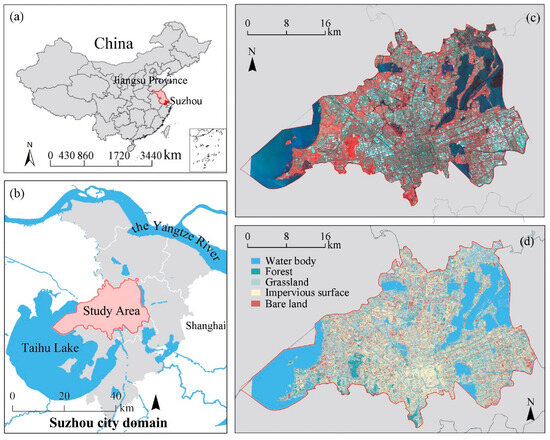
Figure 1.
Maps showing (a) the location of Suzhou city and (b) the study area, (c) GF-1 image of the study areas in 2024 displayed with RGB composition of band 5 (near-infrared), band 4 (red), and band 3 (green); and (d) the land cover map of the study area.
Suzhou was selected as a representative case study for several reasons. First, it is a major city in the Yangtze River Delta region, which is experiencing some of the most rapid urbanization in China, accompanied by strong UHI effects. Second, Suzhou is renowned for its extensive blue-green infrastructure. Approximately 34.6% of its surface area is occupied by interconnected rivers and lakes, ranking it among China’s most water-abundant urban centers [29]. This extensive hydrographic network, integrated with its abundant urban forests [28], provides an ideal landscape to investigate the interactions between water bodies and green spaces, a central objective of this study.
2.2. Land Cover Classification
This study utilized Gaofen-1 (GF-1) satellite data (Scene ID: GF1C_PMS_E120.6_N31.3_20240517_L1A1022254051; Acquisition date: 17 May 2024) for land cover classification. The GF-1 imagery was purchased from the spatial information service provider (Kosmos Remote Sensing Technology Co., Ltd., Beijing, China). The GF-1 satellite is equipped with two types of sensors: a 2 m panchromatic/8 m multispectral camera and a 16 m multispectral wide-field camera, offering both high resolution and wide coverage capabilities (Table 1) [30]. Data preprocessing included radiometric calibration, atmospheric correction, image fusion (to generate 2 m resolution), and clipping to the study area. Subsequently, a Support Vector Machine method was employed to classify the study area into five main categories: forest (trees and tree-dominated land), grassland (grasses and grass-dominated land), water body, impervious surface, and bare land (Figure 1d).

Table 1.
Features of GF-1 images.
Following this, 2299 sample points, uniformly distributed across the study area, were randomly selected for constructing the confusion matrix. High-resolution imagery from Google Earth was visually interpreted to serve as ground reference data. An error matrix (also known as a confusion matrix) was constructed to evaluate the classification accuracy. The overall accuracy was calculated as the percentage of correctly classified sample points out of the total points. The results showed an overall accuracy of 93.13% for the land cover classification. Additionally, producer’s accuracy (PA, measure of omission error) and user’s accuracy (UA, measure of commission error) were calculated for each class (see Table S1). The achieved accuracy meets the requirements of this study. In terms of the cooling effect of green spaces, trees exert the strongest influence, followed by shrubs and grass [31,32], so this study focuses specifically on the cooling effects of urban forests. The land cover classification was performed using the ENVI 5.3 software.
2.3. Calculation of LST and Cooling Intensity
This research employed Land Surface Temperature (LST) data derived from Landsat 8–9 OLI/TIRS Collection 2 Level 2 imagery, which offers a spatial resolution of 30 m (refer to Table 2). This dataset is from the United States Geological Survey (https://glovis.usgs.gov/, accessed on 15 March 2025). The retrieval of LST values relied on the refined Single-Channel Algorithm (SCA) developed by Jiménez-Muñoz et al. [33]. Stored in 16-bit integer format, the retrieval of original floating-point LST values was performed by applying a scale factor and offset to the digital number (DN) of each pixel, implemented through the formula:
LST (K) = DN × scale_factor + offset
Table 2.
Descriptions of the Landsat 8–9 OLI/TIRS C2 L2 images used.
The scale_factor and offset are 0.003418 and 149, respectively. Subsequently, temperatures in kelvin were converted to degrees Celsius using the relation °C = K − 273.15. The resulting distribution of LST values across the study area is illustrated in Figure 2. Same as previous studies [13,32], the cooling intensity was defined as the difference between the regional average temperature (water excluded) and the forest patch average temperature in this study. The calculation of LST and cooling intensity was completed using ENVI and ArcGIS 10.3 software, respectively.
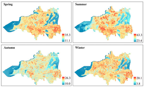
Figure 2.
LST distribution map of the study area for spring, summer, autumn, and winter. LST unit: °C.
2.4. Selections and Definitions of Landscape Indicators
Based on previous research, data availability, and relevance to urban planning, six landscape metrics were selected to quantify the spatial characteristics, vegetation abundance, and surrounding landscape composition of forest patches. Specifically, patch area (Area) and shape index (SHAPE = perimeter/2)) were used to describe spatial characteristics [13,34]. The SHAPE index equals 1 for a maximally compact patch (e.g., a circle) and increases with greater shape irregularity. The mean Normalized Difference Vegetation Index (NDVI) within each forest patch, derived from the 8 m resolution GF-1 multispectral imagery, was selected to represent vegetation density [35]. To characterize the neighboring landscape of each patch, the percentage of neighboring water bodies (NWP) and neighboring greenspace (NGP) within a defined buffer was calculated [31]. Existing studies suggest that the cooling distance of a green space is comparable to the radius of a circle of equivalent area [36,37]. Thus, a buffer zone equal to this cooling distance was established, and NWP and NGP were defined as the ratio of water or greenspace area to the total area within the buffer zone surrounding the forest patch. Elevation, obtained from the 30 m resolution ALOS DEM and included as a natural factor largely beyond human control, served as a control variable and is not discussed further in the analysis. All patch area and perimeter measurements were calculated from the forest vector data using the ArcMap platform. Since the LST data had a spatial resolution of 30 m × 30 m (0.09 ha per pixel) (see Table S2), forest patches smaller than 1 ha were excluded from the analysis.
2.5. XGBoost-SHAP Interpretable Machine Learning Framework
This study employs XGBoost regression [27] combined with SHAP (SHapley Additive exPlanations) analysis to examine the non-linear relationships and interaction effects between landscape variables and the cooling intensity of forest patches across four seasons. XGBoost was selected for this study due to its proven capability to model complex, high-dimensional non-linear relationships, which often leads to superior predictive accuracy and robustness compared to alternatives like Random Forest [38]. This performance is achieved through its additive tree ensembles and advanced regularization techniques, which effectively prevent overfitting. Furthermore, XGBoost offers several key practical advantages, including high computational efficiency through parallel processing, automatic handling of missing values, and robustness to outliers. Finally, its computational efficiency facilitates the advanced interpretability analyses that are critical for this study. The SHAP framework was applied to interpret the model predictions, quantifying the marginal contribution of each landscape feature while accounting for potential interaction effects. A positive SHAP value indicates a feature increases the predicted cooling intensity, while a negative value indicates a decrease. Note that SHAP analysis is performed on the trained model and does not assume linearity or independence among features, making it suitable for capturing complex relationships even in the presence of moderate collinearity.
The dataset was split into 80% for training and 20% for testing, with the test set reserved exclusively for final validation. Model hyperparameters were optimized using the Optuna framework with Bayesian optimization and five-fold cross-validation on the training set. Consistent random seeds were used throughout to ensure reproducibility. The tuned hyperparameters included n_estimators, max_depth, reg_lambda, min_child_weight, subsample, and learning_rate. The final model was retrained on the full training set using the optimal configuration and evaluated on the held-out test set. All analyses were implemented in Python 3.12.7 using the XGBoost and Optuna libraries.
3. Results
3.1. Basic Information on Cooling Intensity and Model Validation
As shown in Figure 3, the average cooling intensity of forest patches varies significantly across seasons. Summer exhibits the highest mean cooling level, followed by spring and autumn, with winter showing the lowest values. Similarly, the heterogeneity level of cooling intensity among patches is strongest in summer (ranging from −5.67 °C to 10.05 °C), followed by spring (−4.04 °C to 4.85 °C). Autumn (−2.43 °C to 3.69 °C) and winter (−2.48 °C to 2.71 °C) demonstrate the weakest heterogeneity. The majority of cooling intensity values in summer fall within the 2–6 °C range, while spring, autumn, and winter predominantly show cooling intensity concentrations in the 0–2 °C interval.
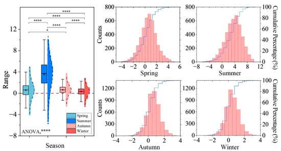
Figure 3.
Seasonal distribution of cooling intensity (°C) for urban forests. Significance levels were determined using independent-samples t-tests; **** denotes p < 0.001 and * denotes p < 0.05.
Based on the modeling results using XGBoost combined with SHAP analysis (Table 3), the predictive model for cooling intensity of forest patches exhibits significant seasonal performance variations. During summer, cooling intensity shows the largest range (range = 15.72 °C). Despite its relatively high absolute error (RMSE = 1.609), this represents only 10.2% of the total variation span. Coupled with the strongest explanatory power (R2 = 0.609), this indicates that the selected feature variables effectively capture the cooling mechanisms for summer. In winter, while absolute error is the lowest (RMSE = 0.641), the narrow cooling range (range = 5.19 °C) results in an error proportion of 12.3%. When combined with the weakest explanatory power (R2 = 0.307), this highlights the current features’ insufficient capacity to explain the heterogeneity in cooling intensity among forest patches during winter. Spring demonstrates an intermediate cooling range (range = 8.89 °C). The testing set RMSE of 1.014 accounts for 11.4% of the variation range, aligning with its moderate explanatory power (R2 = 0.439). Autumn has the smallest cooling range (range = 6.12 °C), with an RMSE of 0.668 representing 10.9% of the variation. However, its explanatory power (R2 = 0.324) is significantly lower than summer’s, suggesting that NDVI-dominated cooling mechanisms in autumn are not fully characterized. Notably, the seasonal ranking of error proportion (Winter > Spring ≈ Autumn > Summer) is inversely related to the R2 ranking (Summer > Spring > Autumn > Winter), confirming that the model demonstrates superior explanatory capability during seasons with greater cooling magnitudes.
Table 3.
Overall model accuracy.
3.2. Identification of Dominant Drivers and Non-Linear Threshold Effect
The influencing factors on the cooling intensity of forest patches exhibit significant seasonal variations (Figure 4). During spring, NWP serves as the core driver of the cooling effect, exerting a substantially stronger influence than all other factors. This is followed by NGP, NDVI, and Elevation, which demonstrate comparable significance. In contrast, patch AREA and SHAPE exert relatively weaker influences. In summer, NWP remains the most critical driver, followed by NDVI and NGP, which hold similar importance. AREA exerts a discernible influence, while the contributions of Elevation and SHAPE are comparatively minor. In autumn, NDVI emerges as the most dominant driver, succeeded by NGP, NWP, AREA, Elevation, and SHAPE in order of declining influence. Winter again features NWP as the core driver, with NDVI ranking next in importance. Elevation and SHAPE then follow, demonstrating comparable significance, while NGP and AREA exhibit relatively weaker impacts during this season.
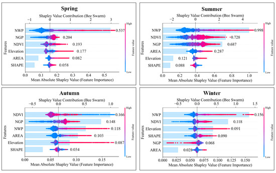
Figure 4.
Seasonal predictor importance and its directional effects on the cooling intensity of urban forests.
As shown in Figure 5, the relationships between forest landscape metrics and their cooling intensity are non-linear and exhibit significant seasonal threshold effects. Specifically, the impacts of NWP, AREA, and Elevation on forest patch cooling intensity demonstrate consistent overall trends across all four seasons, differing primarily in the magnitudes of their seasonal thresholds. Cooling intensity increases linearly with rising NWP, but this effect becomes statistically significant (SHAP > 0) only after exceeding seasonal critical thresholds (Spring: 11%, Summer: 12%, Autumn: 15%, Winter: 12%). Below these thresholds, its cooling effect is susceptible to interaction influences. For patch area, cooling intensity exhibits logarithmic growth with increasing size, with its enhancing effect on cooling becoming significant (SHAP > 0) only after surpassing seasonal critical thresholds (Spring: 2.74 ha, Summer: 2.33 ha, Autumn: 2.48 ha, Winter: 6.73 ha). Furthermore, the positive influence on cooling intensity tapers off after exceeding a saturation threshold (Spring: 12 ha, Summer: 12 ha, Autumn: 12 ha, Winter: 14 ha). Similarly, cooling intensity increases logarithmically with rising Elevation, and its significant positive effect (SHAP > 0) emerges only after exceeding seasonal critical thresholds (Spring: 8.35 m, Summer: 7.81 m, Autumn: 8.28 m, Winter: 7.89 m), plateauing beyond a saturation threshold (approximately 20 m).
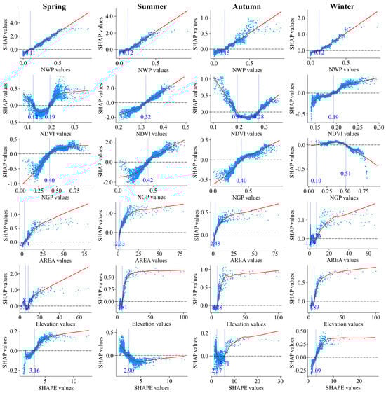
Figure 5.
Seasonal SHAP dependence plots showing the relationship between landscape indicators and cooling intensity.
In contrast, the impacts of NDVI, NGP, and the SHAPE index on forest patch cooling intensity show distinct seasonal variations. An increase in NDVI leads to rising cooling intensity after exceeding critical thresholds (Spring: 0.19; Summer: 0.32; Autumn: 0.28; Winter: 0.19), with this enhancing effect diminishing as NDVI values increase further. The influence of NGP follows similar trends in spring, summer, and autumn, differing only in winter. During spring, summer, and autumn, cooling intensity increases with rising NGP once it surpasses a baseline threshold (25% for all three seasons), but the statistically significant positive effect (SHAP > 0) requires exceeding higher critical thresholds (Spring: 40%, Summer: 42%, Autumn: 40%). In winter, when NGP is low (<37%), its impact on cooling intensity is negligible. Yet, when NGP exceeds 37%, the cooling intensity decreases with further increases in NGP. Seasonal differences for SHAPE are even more pronounced. In spring and winter, cooling intensity strengthens with increasing SHAPE, stabilizing into a consistent positive effect beyond critical thresholds (Spring: 3.16; Winter: 3.09). During summer, SHAPE exerts an overall negative effect on cooling intensity, stabilizing into a consistent negative effect beyond 2.9. In autumn, cooling intensity decreases with rising SHAPE when SHAPE is low (<3.5), but its negative effect weakens and cooling intensity begins to rise when SHAPE exceeds 3.5.
3.3. Interaction and Interaction Thresholds of Landscape Drivers
The impact of NWP on cooling intensity is significantly modulated by NDVI thresholds, demonstrating distinct seasonal patterns (Figure 6 and Table 4). During spring, NWP positively enhances cooling when NDVI ≤ 0.19 but shifts to a negative inhibitory effect when NDVI exceeds this threshold. In summer, the NDVI threshold controlling NWP’s effect increases to 0.32, with NWP enhancing cooling below this value and reducing it above. Winter reverts to the spring threshold of 0.19 with identical effect reversal, whereas autumn shows no significant interaction. In addition, SHAPE functions as a stable regulatory factor with a consistent seasonal threshold of 3.0, though its directional influence varies seasonally. When interacting with NDVI, SHAPE ≤ 3.0 allows NDVI to enhance cooling in spring and autumn, but this effect reverses when SHAPE > 3.0. However, NDVI inhibits cooling at lower SHAPE values (≤3.0) yet promotes it at higher complexity (>3.0) in summer. In its winter interaction with NGP, SHAPE ≤ 3.0 leads to NGP inhibiting cooling, while beyond this threshold, NGP’s effect becomes positive. This indicates that patch shape complexity fundamentally alters vegetation indicators’ cooling efficiency through effect reversal mechanisms.
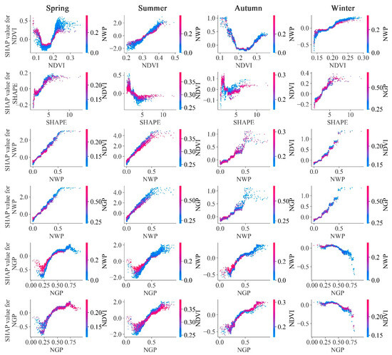
Figure 6.
Interactions between pairwise landscape drivers and their impact on cooling intensity.
Table 4.
Thresholds and effect shifts of pairwise interactions between landscape drivers on cooling intensity.
Both NWP and NGP demonstrate bidirectional regulatory functions. NWP modulates NDVI’s impact such that when NWP ≤ 7% (spring/summer/winter), NDVI enhances cooling, though this benefit diminishes above the threshold. Meanwhile, NWP also regulates NGP. During spring, NGP strengthens cooling at NWP ≤ 15% but reverses direction beyond this point, while summer shows a lower threshold of 10% with identical reversal. Conversely, NGP governs NWP’s effects through seasonal thresholds (NGP = 40% in spring, 48% in summer, 38% in autumn), enhancing cooling below these values but inhibiting it above them. For NDVI regulation, summer demonstrates threshold behavior at NGP = 38% (positive-to-negative reversal), whereas autumn (NGP = 48%) and winter (NGP = 44%) display unique inhibition-to-enhancement reversal patterns where elevated NGP activates NDVI’s cooling potential. No significant NGP-NDVI interaction occurs in spring.
4. Discussion
The landscape variables selected in this study were highly effective in explaining the cooling intensity of forest patches in summer (R2 = 0.615), but demonstrated limited capability in explaining the cooling intensity in autumn (R2 = 0.352) and winter (R2 = 0.316). The core reason is that the cooling processes of vegetation and water bodies in summer are dominated by intense and persistent transpiration and evaporation [39,40,41], which can be captured and characterized by the selected static landscape variables. In contrast, the heterogeneity of cooling effects from forest patches is weaker in autumn and winter (Figure 3), and their cooling processes are likely more driven by synoptic weather dynamics factors (such as wind speed, cloud cover, cold wave frequency), which cannot be captured by the static landscape variables used in this study. The research confirms that the core drivers of forest cooling, their importance, non-linear driving mechanisms, and pairwise interactions all exhibit significant seasonal variations. Consequently, a single optimal greening strategy does not exist. Instead, season-specific strategies are required. During spring, summer, and autumn, the external landscape composition (NWP, NGP) and internal planting density of forest patches are the most critical factors dominating the cooling intensity, while the spatial characteristics of the patches themselves (area and shape) are less important.
In both spring and summer, NWP was the most important driver of the cooling effect of forest patches. This indicates that in seasons with rising temperatures and enhanced evaporation, the local “cool-moist effect” is the primary mechanism driving cooling. Water bodies remove substantial heat through evaporation, lowering the overall ambient air temperature baseline of the surrounding area, thereby establishing the cooling effect of the forest itself on a cooler foundation. This aligns with findings from previous studies [22,23,24], which discovered synergistic cooling effects between adjacent blue and green spaces. This study further confirms that the influence of patch NWP is strongly dependent on the patch’s own vegetation planting density and the scale of neighboring green spaces, with clear interaction thresholds (Table 4). Therefore, it is recommended to prioritize adding water bodies up to the seasonal critical thresholds (Spring: 11%, Summer: 12%, Autumn: 15%, Winter: 12%) near sparse forest patches, and under the precondition that the patch’s NGP is below a certain level (Spring: 40%, Summer: 48%, Autumn: 38%), to ensure a positive effect of neighboring water bodies on the forest patch’s cooling effect, while avoiding additional water body increases from having negative effects.
The high importance of NGP indicates that enhanced cooling effects exist between adjacent green spaces during spring, summer, and autumn, which is consistent with previous research [25,42]. The more green space surrounding a forest patch, the more it can form a contiguous cool area, reduce heat source interference, and enhance the overall cooling capacity. The results suggest that increasing green space coverage around forest patches where NWP is below the interaction threshold (Spring: 15% and Summer: 10%) until NGP reaches the seasonal critical threshold (Spring: 40%, Summer: 42%, Autumn: 40%) can ensure a positive effect of NGP on forest cooling. In winter, however, once NGP exceeds 37%, further increase contributes to thermal insulation through mechanisms such as wind reduction and radiation blocking. This buffering effect inhibits heat loss, thereby reducing the cooling intensity of forest patches. These findings highlight a seasonal contrast: higher NGP enhances cooling in warm seasons but provides insulating effects in winter, demonstrating the dual role of greenspace configuration in regulating thermal environments across different seasons.
The importance of vegetation density (NDVI) for the cooling effect of forest patches is also confirmed, consistent with conclusions from previous studies [12,43,44]. However, this study confirms that NDVI becomes the most critical factor only in autumn, likely because the difference in NDVI between patches dominated by deciduous species (which are losing leaves) and those dominated by evergreen species increases, leading to its heightened importance. The results of this study suggest that greening optimization layouts aimed at thermal environment mitigation should avoid blindly increasing vegetation density. For instance, when the neighboring water body proportion of a patch exceeds a certain threshold (NWP > 7%), reducing planting density to increase ventilation corridors might be more effective than solely planting more trees. In summer, for forest patches with more complex shapes (SHAPE > 3.0), their cooling intensity can be improved by increasing internal vegetation planting density, but this method is not applicable in spring and autumn.
The relationship between patch area and forest cooling intensity follows a logarithmic pattern across all four seasons [13,45]. Beyond a certain threshold (Spring: 12 ha, Summer: 12 ha, Autumn: 12 ha, Winter: 14 ha), the cooling effect essentially saturates, meaning additional area growth does not yield more cooling benefits. Greening optimization measures should prioritize forest patches with areas smaller than the seasonal critical threshold (Spring: 2.74 ha, Summer: 2.33 ha, Autumn: 2.48 ha, Winter: 6.73 ha), as these patches are more susceptible to other influencing factors and their cooling effects are often not guaranteed. This resonates with the conclusions of Zhou et al. [13], whose results suggested that in a subtropical city (Shanghai, adjacent to the study area), a forest patch area exceeding 4 ha inevitably leads to effective cooling, whereas below this threshold, cooling effects are not certain.
The impact of forest patch shape complexity on cooling intensity is not constant, and its direction (positive/negative) and strength depend on the season, and there are clear threshold effects. Summer differs from the other three seasons, as higher geometric shape complexity is associated with lower cooling intensity, which is consistent with previous findings [14,17,46]. This is likely because a more complex shape implies a higher edge-to-area ratio, meaning more of the forest is exposed to the edge, making the entire patch more susceptible to penetration by the external thermal environment, which is not conducive to forming a stable cool core. Furthermore, when complexity exceeds a certain threshold (Summer > 4.40), shape no longer has a significant influence on the patch’s cooling effect. In cooler seasons, more complex patches are more beneficial for forests to exert cooling benefits, possibly because complex boundaries can enhance wind protection and better retain cold air, thereby increasing the cooling intensity of the forest patch. This, to some extent, explains the inconsistent findings regarding the impact of shape index on the cooling intensity of green space patches in existing studies.
This study has several limitations. The findings are site-specific due to influences from local climate, vegetation structure, geographic conditions, and data resolution, limiting their direct applicability to other regions. Furthermore, the reliance on static landscape metrics and the inability to incorporate dynamic meteorological factors (e.g., wind speed, humidity) represent another constraint, as these elements critically regulate cooling efficiency. The use of multi-year satellite imagery (2021–2024) also introduced unresolved interannual hydroclimatic variations. Future research should address these gaps by integrating high-resolution vegetation structural data (e.g., LiDAR), repeating similar analyses across diverse climatic zones, and combining multi-source satellite imagery with meteorological models (e.g., WRF) to better isolate temporal and climatic influences. Higher-frequency satellite data (e.g., Sentinel-2) could further help quantify short-term hydrological and thermal dynamics.
5. Conclusions
This study reveals that the driving mechanisms behind the cooling effect of urban forest patches are highly complex and seasonally heterogeneous. The strong evapotranspiration in summer allows static landscape variables to effectively explain variations in cooling intensity, while cooling in autumn and winter is more dominated by dynamic meteorological factors, leading to diminished model explanatory power. A core finding is that a universal optimal greening strategy does not exist, and planning practices must be season-specific. During warmer seasons (spring, summer, autumn), emphasis should be placed on optimizing the external spatial configuration of forest patches—prioritizing enhanced proximity to water bodies and adjacent green spaces to maximize their synergistic cooling effects. Simultaneously, adjustments to internal vegetation density must consider interaction thresholds with external factors. In cold winters, adjacent green spaces demonstrate insulating services through wind blocking and radiation reduction. Furthermore, the patch area exhibits a clear saturation threshold, suggesting priority should be given to caring for and optimizing small and medium-sized patches. The influence of patch shape varies by season, underscoring its dual-sided and complex role. Therefore, future urban green space planning and design should move beyond single-mode approaches and adopt a dynamic, precise adaptive management framework. This framework should comprehensively consider the dominant mechanisms and key thresholds across different seasons to holistically enhance the year-round ecosystem service efficiency of green spaces.
Supplementary Materials
The following supporting information can be downloaded at: https://www.mdpi.com/article/10.3390/f16101514/s1, Table S1: Error matrix and accuracy assessment for the land cover classification; Table S2: Band information of Landsat 8/9 Operational Land Imager (OLI) and Thermal Infrared Sensor (TIRS).
Author Contributions
Conceptualization, Y.Z., R.Z. and W.Z.; Methodology, Y.Z., Y.Y., K.P. and R.Z.; Software, Y.Z., Y.Y. and K.P.; Validation, Y.Y. and K.P.; Resources, W.Z.; Data curation, Y.Z.; Writing—original draft, Y.Z. and Y.Y.; Writing—review & editing, K.P., R.Z. and W.Z.; Visualization, Y.Z. and R.Z.; Supervision, W.Z. All authors have read and agreed to the published version of the manuscript.
Funding
This research was funded by the National Natural Science Foundation of China (Grant Number: 32101577; 32401660) and Scientific Research Foundation for Advanced Talents, Yangzhou University (Grant Number: 137012167).
Data Availability Statement
The data presented in this study are available on request from the corresponding author.
Conflicts of Interest
The authors declare no conflict of interest.
References
- Gogoi, P.P.; Vinoj, V.; Swain, D.; Roberts, G.; Dash, J.; Tripathy, S. Land use and land cover change effect on surface temperature over Eastern India. Sci. Rep. 2019, 9, 8859. [Google Scholar] [CrossRef] [PubMed]
- Dadashpoor, H.; Azizi, P.; Moghadasi, M. Land use change, urbanization, and change in landscape pattern in a metropolitan area. Sci. Total Environ. 2019, 655, 707–719. [Google Scholar] [CrossRef] [PubMed]
- Stewart, I.D.; Oke, T.R. Local Climate Zones for Urban Temperature Studies. Bull. Am. Meteorol. Soc. 2003, 86, 370–384. [Google Scholar] [CrossRef]
- Anderson, G.B.; Michelle, L. Bell Heat waves in the United States: Mortality risk during heat waves and effect modification by heat wave characteristics in 43 US communities. Environ. Health Perspect. 2011, 119, 210–218. [Google Scholar] [CrossRef]
- Mora, C.; Dousset, B.; Caldwell, I.R.; Powell, F.E.; Geronimo, R.C. Global risk of deadly heat. Nat. Clim. Change 2017, 7, 501–506. [Google Scholar] [CrossRef]
- Kusaka, H.; Hara, M.; Takane, Y. Urban climate projection by the WRF model at 3 km horizontal grid increment: Dynamical downscaling and predicting heat stress in the 2070’s August for Tokyo, Osaka, and Nagoya. J. Meteorol. Soc. Japan 2012, 90b, 47–63. [Google Scholar] [CrossRef]
- Walter V Reid Biodiversity hotspots. Trends Ecol. Evol. 1998, 13, 275–280. [CrossRef]
- IPCC. AR6 Synthesis Report Climate Change 2023; IPCC: Geneva, Switzerland, 2023. [Google Scholar]
- Santamouris, M.; Ban-Weiss, G.; Osmond, P.; Paolini, R. Progress in urban greenery mitigation science–assessment methodologies advanced technologies and impact on cities. J. Civ. Eng. Manag. 2018, 24, 638–671. [Google Scholar] [CrossRef]
- Yu, Z.; Guo, X.; Zeng, Y.; Koga, M.; Vejre, H. Variations in land surface temperature and cooling efficiency of green space in rapid urbanization: The case of Fuzhou city, China. Urban For. Urban Green. 2018, 29, 113–121. [Google Scholar] [CrossRef]
- Bonan, G.B. Forests and Climate Change: Forcings, Feedbacks, and the Climate Benefits of Forests. Science 2008, 320, 1444–1449. [Google Scholar] [CrossRef] [PubMed]
- Schwaab, J.; Meier, R.; Mussetti, G.; Seneviratne, S.; Bürgi, C.; Davin, E.L. The role of urban trees in reducing land surface temperatures in European cities. Nat. Commun. 2021, 12, 6763. [Google Scholar] [CrossRef]
- Zhou, W.; Yu, W.; Zhang, Z.; Cao, W.; Wu, T. How can urban green spaces be planned to mitigate urban heat island effect under different climatic backgrounds? A threshold-based perspective. Sci. Total Environ. 2023, 890, 164422. [Google Scholar] [CrossRef]
- Du, H.; Song, X.; Jiang, H.; Kan, Z.; Wang, Z.; Cai, Y. Research on the cooling island effects of water body: A case study of Shanghai, China. Ecol. Indic. 2016, 67, 31–38. [Google Scholar] [CrossRef]
- Peng, J.; Dan, Y.; Qiao, R.; Liu, Y.; Dong, J.; Wu, J. How to quantify the cooling effect of urban parks? Linking maximum and accumulation perspectives. Remote Sens. Environ. 2021, 252, 112135. [Google Scholar] [CrossRef]
- Yu, Z.; Yang, G.; Zuo, S.; Jørgensen, G.; Koga, M.; Vejre, H. Critical review on the cooling effect of urban blue-green space: A threshold-size perspective. Urban For. Urban Green. 2020, 49, 126630. [Google Scholar] [CrossRef]
- Feyisa, G.L.; Dons, K.; Meilby, H. Efficiency of parks in mitigating urban heat island effect: An example from Addis Ababa. Landsc. Urban Plan. 2014, 123, 87–95. [Google Scholar] [CrossRef]
- Masoudi, M.; Tan, P.Y. Multi-year comparison of the effects of spatial pattern of urban green spaces on urban land surface temperature. Landsc. Urban Plan. 2019, 184, 44–58. [Google Scholar] [CrossRef]
- Chen, A.; Yao, X.A.; Sun, R.; Chen, L. Effect of urban green patterns on surface urban cool islands and its seasonal variations. Urban For. Urban Green. 2014, 13, 646–654. [Google Scholar] [CrossRef]
- Dugord, P.-A.; Lauf, S.; Schuster, C.; Kleinschmit, B. Land use patterns, temperature distribution, and potential heat stress risk—the case study Berlin, Germany. Comput. Environ. Urban Syst. 2014, 48, 86–98. [Google Scholar] [CrossRef]
- Du, H.; Cai, W.; Xu, Y.; Wang, Z.; Wang, Y.; Cai, Y. Quantifying the cool island effects of urban green spaces using remote sensing Data. Urban For. Urban Green. 2017, 27, 24–31. [Google Scholar] [CrossRef]
- Zhou, W.; Cao, W.; Wu, T.; Zhang, T. The win-win interaction between integrated blue and green space on urban cooling. Sci. Total Environ. 2023, 863, 160712. [Google Scholar] [CrossRef]
- Fei, F.; Wang, Y.; Yao, W.; Gao, W.; Wang, L. Coupling mechanism of water and greenery on summer thermal environment of waterfront space in China’s cold regions. Build. Environ. 2022, 214, 108912. [Google Scholar] [CrossRef]
- Shi, D.; Song, J.; Huang, J.; Zhuang, C.; Guo, R.; Gao, Y. Synergistic cooling effects (SCEs) of urban green-blue spaces on local thermal environment: A case study in Chongqing, China. Sustain. Cities Soc. 2020, 55, 102065. [Google Scholar] [CrossRef]
- Geng, X.; Yu, Z.; Zhang, D.; Li, C.; Yuan, Y.; Wang, X. The influence of local background climate on the dominant factors and threshold-size of the cooling effect of urban parks. Sci. Total Environ. 2022, 823, 153806. [Google Scholar] [CrossRef]
- Masoudi, M.; Tan, P.Y.; Fadaei, M. The effects of land use on spatial pattern of urban green spaces and their cooling ability. Urban Clim. 2021, 35, 100743. [Google Scholar] [CrossRef]
- Chen, T.; Guestrin, C. XGBoost: A scalable tree boosting system. In Proceedings of the ACM SIGKDD International Conference on Knowledge Discovery and Data Mining, San Francisco, CA, USA, 13–17 August 2016; Association for Computing Machinery: New York, NY, USA, 2016; pp. 785–794. [Google Scholar]
- Suzhou Local Chronicles Compilation Office Suzhou Chronicles: Nature Environment. Available online: https://dfzb.suzhou.gov.cn/dfzb/jzyg/202411/fadda033bf744f669a446dd40103f180.shtml (accessed on 6 May 2024). (In Chinese)
- Suzhou Municipal Bureau Statistics Suzhou Statistical Yearbook 2023. Available online: https://tjj.sh.gov.cn/tjnj/20250331/9f8ec62cc2234485b0aa411b8d967c37.html (accessed on 6 May 2024). (In Chinese)
- Natural Resources Satellite Remote Sensing Cloud Service Platform: Gaofen-1 Satellite. Available online: http://114.116.226.59/chinese/satellite/chinese/gf1 (accessed on 6 September 2025). (In Chinese).
- Zhou, W.; Yu, W.; Wu, T. An alternative method of developing landscape strategies for urban cooling: A threshold-based perspective. Landsc. Urban Plan. 2022, 225, 104449. [Google Scholar] [CrossRef]
- Kong, F.; Yin, H.; James, P.; Hutyra, L.R.; He, H.S. Effects of spatial pattern of greenspace on urban cooling in a large metropolitan area of eastern China. Landsc. Urban Plan. 2014, 128, 35–47. [Google Scholar] [CrossRef]
- Jiménez-Muñoz, J.C.; Sobrino, J.A.; Skoković, D.; Mattar, C.; Cristóbal, J. Land surface temperature retrieval methods from Landsat-8 thermal infrared sensor data. IEEE Geosci. Remote Sens. Lett. 2014, 11, 1840–1843. [Google Scholar] [CrossRef]
- McGarial, K.; Marks, B. FRAGSTAT: Spatial Pattern Analysis Program for Quantifying Landscape Structure; U.S. Department of Agriculture Forest Service: Washington, DC, USA, 1995.
- Valor, E.; Caselles, V. Mapping land surface emissivity from NDVI: Application to European, African, and South American areas. Remote Sens. Environ. 1996, 57, 167–184. [Google Scholar] [CrossRef]
- Xiao, Y.; Piao, Y.; Pan, C.; Lee, D.; Zhao, B. Using buffer analysis to determine urban park cooling intensity: Five estimation methods for Nanjing, China. Sci. Total Environ. 2023, 868, 161463. [Google Scholar] [CrossRef]
- Chang, C.-R.; Li, M.-H.; Chang, S.-D. A preliminary study on the local cool-island intensity of Taipei city parks. Landsc. Urban Plan. 2007, 80, 386–395. [Google Scholar] [CrossRef]
- Joharestani, M.Z.; Cao, C.; Ni, X.; Bashir, B.; Talebiesfandarani, S. PM2.5 Prediction based on random forest, XGBoost, and Deep learning using multisource remote sensing data. Atmosphere 2019, 10, 373. [Google Scholar] [CrossRef]
- Gunawardena, K.R.; Wells, M.J.; Kershaw, T. Utilising green and bluespace to mitigate urban heat island intensity. Sci. Total Environ. 2017, 584–585, 1040–1055. [Google Scholar] [CrossRef] [PubMed]
- Rahman, M.A.; Moser, A.; Rötzer, T.; Pauleit, S. Microclimatic differences and their influence on transpirational cooling of Tilia cordata in two contrasting street canyons in Munich, Germany. Agric. For. Meteorol. 2017, 232, 443–456. [Google Scholar] [CrossRef]
- Manteghi, G.; Limit, H.; Remaz, D. Water bodies an urban microclimate: A Review. Mod. Appl. Sci. 2015, 9, 1. [Google Scholar] [CrossRef]
- Liao, W.; Guldmann, J.-M.; Hu, L.; Cao, Q.; Gan, D.; Li, X. Linking urban park cool island effects to the landscape patterns inside and outside the park: A simultaneous equation modeling approach. Landsc. Urban Plan. 2023, 232, 104681. [Google Scholar] [CrossRef]
- Weng, Q. A remote sensing-GIS evaluation of urban expansion and its impact on surface temperature in the Zhujiang Delta, China. Int. J. Remote Sens. 2001, 22, 1999–2014. [Google Scholar] [CrossRef]
- Zhang, X.; Zhong, T.; Feng, X.; Wang, K. Estimation of the relationship between vegetation patches and urban land surface temperature with remote sensing. Int. J. Remote Sens. 2009, 30, 2105–2118. [Google Scholar] [CrossRef]
- Yang, G.; Yu, Z.; Jørgensen, G.; Vejre, H. How can urban blue-green space be planned for climate adaption in high-latitude cities? A seasonal perspective. Sustain. Cities Soc. 2020, 53, 101932. [Google Scholar] [CrossRef]
- Zhou, W.; Cao, F.; Wang, G. Effects of spatial pattern of forest vegetation on urban cooling in a compact megacity. Forests 2019, 10, 282. [Google Scholar] [CrossRef]
Disclaimer/Publisher’s Note: The statements, opinions and data contained in all publications are solely those of the individual author(s) and contributor(s) and not of MDPI and/or the editor(s). MDPI and/or the editor(s) disclaim responsibility for any injury to people or property resulting from any ideas, methods, instructions or products referred to in the content. |
© 2025 by the authors. Licensee MDPI, Basel, Switzerland. This article is an open access article distributed under the terms and conditions of the Creative Commons Attribution (CC BY) license (https://creativecommons.org/licenses/by/4.0/).