Fitting and Evaluating Taper Functions to Predict Upper Stem Diameter of Planted Teak (Tectona grandis L.f.) in Eastern and Central Regions of Nepal

Abstract

Teak [Tectona grandis L.f.] has a wide distribution range in tropical countries and is Nepal’s second most planted commercial tree species. This study aimed to develop a robust and reliable taper equation for Teak species in Nepal. To achieve this, 15 parametric taper equations were fitted and evaluated using the diameter and height data of 100 trees sampled from two stands of the Sagarnath Plantation projects, Nepal. The data set was split into training (90%) and testing (10%) sets based on the trees’ ID, and model fitting was conducted in two phases. In the first phase, nonlinear models were fitted to the training data using 10-fold cross-validation, and the performance was evaluated based on fit and validation statistics. The top five models were further analyzed in the second phase using a mixed effects framework to account for variance and correlation structures. The modified Bi model performed best under a fixed effects modeling framework (R² = 0.96, RMSE = 1.83 cm). However, the Sharma and Zhang model performed the best under a mixed-effects modeling framework (R² = 0.97, RMSE = 1.54 cm). Therefore, we suggest using the modified Bi under fixed effects and variable exponent equation of Sharma and Zhang under mixed-effects modeling as a taper equation for Teak. The Sharma and Zhang’s equation is recommended for its high accuracy and better performance over previously recommended variable exponents equations.

1. Introduction

Accurate estimation of volume at any specific height and diameter is a crucial component of growth and yield estimation [1]. Individual tree stem volume estimation is critical in determining forest biomass and quantifying carbon stocks [2,3]. Taper equations offer flexibility in representing the stem diameter inside and outside bark and have the advantage of estimating the tree diameter and volume of the tree at any specific height or in the log section [4,5]. The taper equations also provide a framework to incorporate quality attributes into growth and the yield models and decision support system [6,7]. Therefore, several taper equations with varying complexity have been developed for a broad range of species and locations [5,8,9,10,11]. Parametric taper functions are commonly developed and used to predict the diameter of a tree stem at any height of interest [12,13,14]. In a systematic review of taper equations, MCTague and Weiskittel [15] categorized these equations into six categories based on the complexity of model forms: (i) simple polynomial, (ii) segmented, (iii) compatible, (iv) variable forms, (v) trigonometric, and (vi) matrix.

In addition to parametric models, semiparametric and nonparametric models have also been developed to model stem tapering. For example, Zapata-Cuartas et al. [16] and Scolforo et al. [17] employed penalized spline regression to estimate the tapering of the loblolly pine and Brazilian eucalyptus stem, respectively. They reported an improvement in the performance of semiparametric models (penalized spline) over parametric models. With advancements in artificial intelligence, machine learning (ML) models are employed to predict upper stem diameter (e.g., [18,19,20,21]). Although improved performance of nonparametric and semiparametric models based on ML has been reported, they tend to be highly data sensitive, producing overoptimistic results due to overfitting, cannot extend beyond the range of observed data, and often fail to explain the underlying biological processes [15,19]. This underscores the importance and relevance of parametric models over semiparametric and nonparametric models.

Taper data often comes from several sampling plots representing different densities, hierarchical structures, management regimes, or locations [13,22,23,24]. More importantly, these data can have measurement errors [25]. Thus, studies on taper modeling (or forest biometrics) have rendered significant efforts in selecting the best-performing models based on the principles of parsimony, fit and validation statistics, and model simplicity [4,8,26]. Traditionally, fit and validation statistics are calculated by randomly splitting data into training and validation data sets. This serves two purposes: (a) to test the robustness of a model [19] and (b) to evaluate the model performances (e.g., [4,27]). In stem taper modeling, a large body of research has used leave-one-out cross-validation (LOOCV) to explore model performance [16,28,29,30]. However, LOOCV is prone to poor bias–variance trade-offs, sensitive to outliers, and may provide inconsistent performance for nonlinear models [31,32]. As the validation data set should typically resemble the future unseen data set, implementing the cross-validation method should provide a realistic scenario to test the robustness [19]. The k-fold cross-validation methods used in the model validation procedure address the limitation of LOOCV and help to increase the robustness of the model selection process [31,32]. However, when splitting the data, careful consideration should ensure that trees from all diameter classes are represented in the training and validation sets [19]. This approach prevents bias and ensures that the model can generalize across the diameter class, leading to more accurate and reliable predictions. The 5- and 10-fold cross-validations are generally used to evaluate and select empirical growth and yield system models depending on the sample size (e.g., [18,33,34]).

In addition to the cross-validation approach, the implementation of a mixed effects model framework would provide robustness to explain unobserved variability [24,34,35,36]. Fixed effects in these models account for the trend (mean-specific response), and random effects capture the subject-specific response, such as variability within trees, between trees, or between stands [37,38]. Additionally, the incorporation of variance and correlation functions in mixed-effects modeling allows us to account for non-homogeneous variance structures and inherent autocorrelation in parametric regression assumptions [24,29,39,40]. However, the calibration procedure of mixed effects models is generally ignored in forest modeling and coefficient of fixed effects parts is used for model prediction [24,41].

Teak (Tectona grandis Linn F.) is a commercially important species in natural and plantation forests. Teak is a native tree in India, Myanmar, Thailand, and Laos in South and Southeast Asia [42]. Due to its higher commercial value, it is planted outside its natural range in tropical areas of Asia, Africa, and Latin America. The planted Teak forests cover approximately 4.35 to 6.89 million ha in the tropical regions of Asia (80%), Africa (10%), and America (6%) [43]. Myanmar occupies the largest natural Teak forest, covering approximately half of the worldwide natural Teak forests (~29 million ha) [43]. Teak species usually have higher growth rates, larger heartwood proportions, higher wood quality traits (higher density and mechanical strength), better esthetics, and natural durability than other hardwood species [44]. Due to these desirable properties, Teak has become one of the most commercially adopted species of timber plantations worldwide [43]. In Nepal, Teak was introduced in 1978 as an exotic plantation wood species to restore degraded mixed hardwood forests through government initiatives under the Sagarnath Development Project (SDP) [45]. Teak is the second most common plantation species after Eucalyptus in Nepal [30].

Although Teak trees are commercially important species with larger buttresses and higher tapering, little attention is paid to model stem forms and the buttress of planted Teak forests. Documented studies are limited to fewer taper functions [46,47,48], such as Goodwin [48], who developed cubic polynomial taper functions to estimate the upper stem diameter of Teak plantations in Thailand. Subsequent studies compared the Goodwin [48] function with the variable exponent function of Kozak [4] (e.g., [28,49,50]). Koirala et al. [30] attempted to increase the number of functions to predict the upper stem diameter of Teak plantation trees in Nepal by picking top-performing taper equations across different species. In this study, we extended the model forms diversity, picking the best-performing taper models of tropical trees (e.g., [4,14,22,51,52,53]). Given the heterogeneous nature of Teak tapering and larger buttresses, we increased the sample size from previous studies to find the best-performing taper equations for planted Teak species in Nepal. Specifically, the study aimed to compare the multiple types of taper functions to select and offer a robust model that performs better and to compare the results with the existing taper equation developed from dynamic taper function [53] for Teak plantations in Nepal suggested by Koirala et al. [30].

2. Materials and Methods

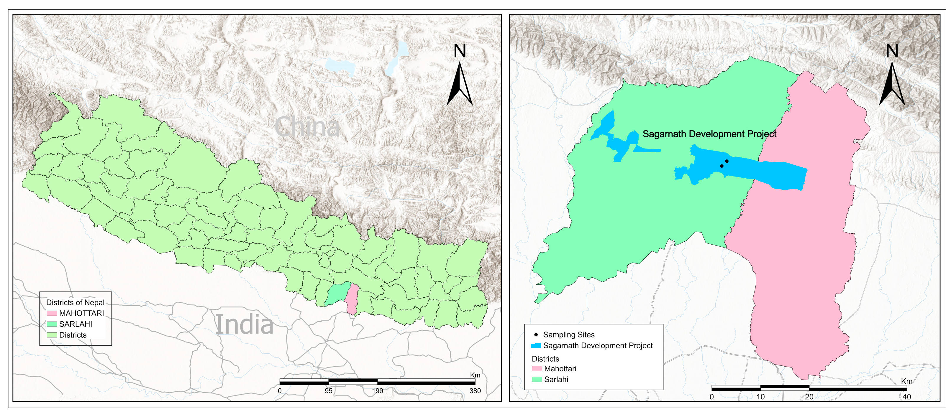
2.1. Study Area

The data set used in this study was collected from the Teak plantation forest of the Sagarnath Development Project (SDP; 26.9974° N and 85.6749° E), Nepal (Figure 1). The SDP was established in 1978 to introduce fast-growing exotic species by replacing degraded mixed hardwood forests in the lowlands of Nepal [45]. The plantation project covers 13,512 hectares and extends over three districts: Sarlahi (52%), Mahottari (46%), and Rautahat (2%). Elevation in the SDP ranges from 60 m above sea level (asl) to 330 m asl (http://sfdp.mofe.gov.np/contents/2; accessed on 10 November 2024). The average summer temperature (June–October) ranges from 35 °C to 45 °C, and the winter temperature can reach as low as 10 °C [54]. The area receives the majority of the precipitation in the form of summer rain, and it varies from 1130 mm to 2680 mm [54]. The area is prone to flooding every year in the monsoon season (June–October), and the soil is weakly developed with eroded gravel and boulders. Teak is the second-most planted timber species after eucalyptus in the SDP, with a mean annual increment (MAI) of 8 m³ ha⁻¹ and a rotation period of 40 years [55].

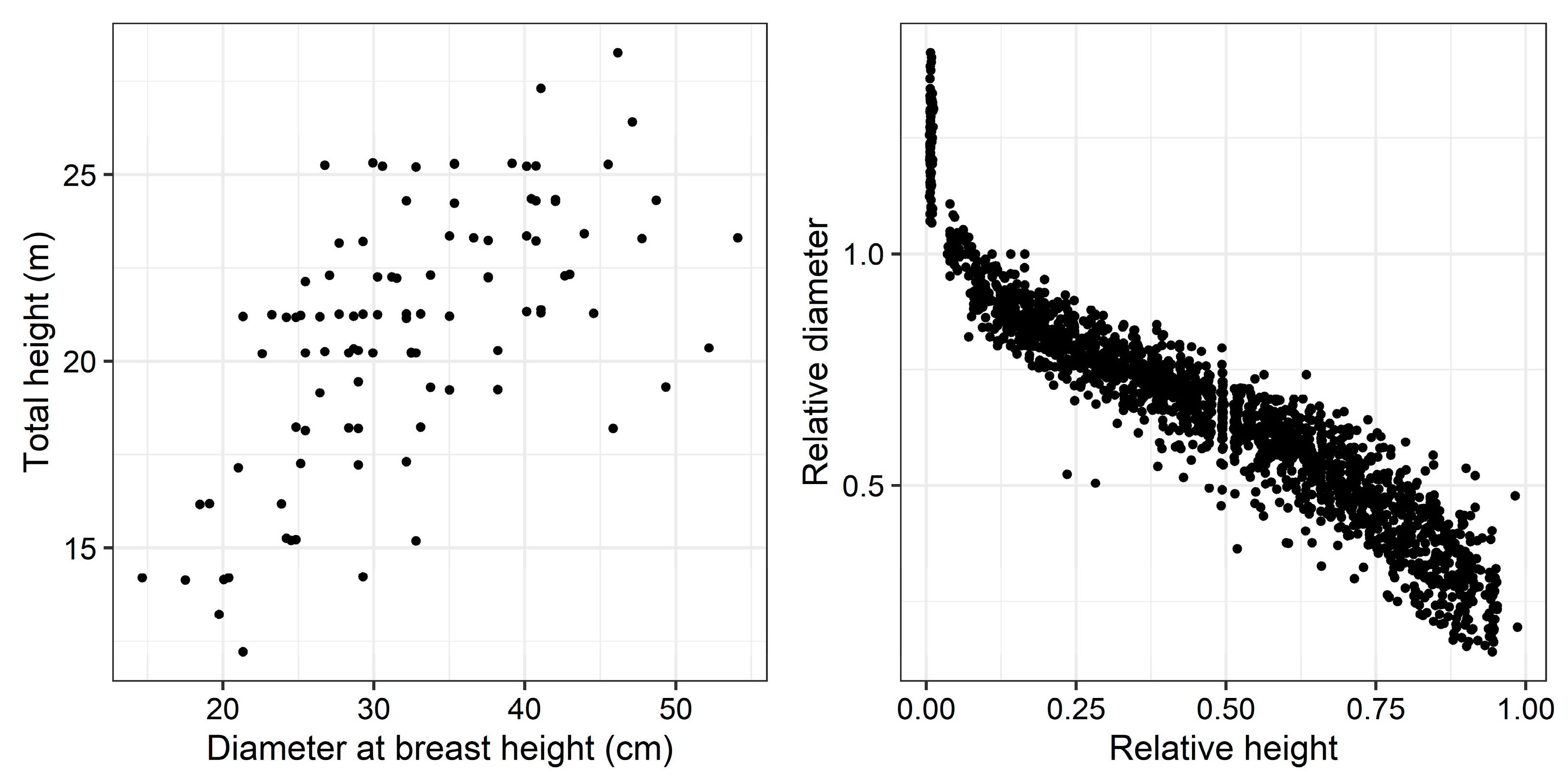
2.2. Sampling and Measurements

The sampling was carried out in two sub-compartments (2D and 1A2) that were ready for final harvesting in 2022. Sub-compartments 2D and 1A2 had a total area of 25 ha and 2.6 ha, respectively, and these sub-compartments were planted in the same year and underwent similar management practices. Of 25 ha, only 7.74 ha, with a total tree of 1435 (185 trees ha⁻¹), was allocated for felling, whereas the entire 1A2 was allocated for clear felling (596 trees; 229 trees ha⁻¹). From the area designated for felling, 50 trees from each sub-compartment having straight bole with no visual defects or deformity were selected across their diameter at breast height (D; measured at 1.3 m from the ground) range. The selected trees were felled, delimbed, and marked at every meter up to a merchantable height (7.5 cm diameter over bark (d)). At each marked location, the dob was recorded. The total height of the tree was measured by adding stump height and total section length. The average D and height of the sample trees were 33.48 cm (standard deviation (sd) = 8.23) and 21.43 m (sd = 3.23). The summary statistics of the trees sampled by diameter category based on D are provided in

Table 1. Summary statistics of the sampled trees. The diameter at breast height (D) is reported in cm, and the total height (H) by diameter class is reported in meters with precision at the centimeter level.

Diameter Class	n	D (cm)			H (m)
(cm)		Mean ± sd	Min	Max	Mean ± sd	Min	Max
<25	19	21.84 ± 2.73	14.64	24.83	17.15 ± 3.01	12.22	21.25
25–30	25	27.71 ± 1.54	25.15	29.92	20.77 ± 2.40	14.23	25.32
30–35	18	32.14 ± 1.06	30.24	33.74	21.4 ± 2.44	15.19	25.23
35–40	13	36.58 ± 1.45	35.01	39.15	22.87 ± 2.04	19.24	25.31
40+	25	43.96 ± 3.86	40.11	54.11	23.58 ± 2.30	18.21	28.27
Overall	100	33.48 ± 8.23	14.64	54.11	21.43 ± 3.23	12.22	28.27

. The plot of total height versus D and relative height (section height (h) divided by total height (H); [h/H]) versus relative diameter (section diameter over diameter at breast height; [d/D]) are shown in Figure 2.

2.3. Taper Equations

Fifteen taper equations previously used to estimate the upper stem diameter of various tropical tree species were selected to evaluate the tapering of Teak species (

Table 2. Selected taper model forms and their designations.

Model	Equations	Authors
M1	${\displaystyle \frac{{\mathrm{d}}^2}{{\mathrm{D}}^2}}={\mathsf{\beta }}_1\left({\displaystyle \frac{\mathrm{h}}{\mathrm{H}}}-1\right)+{\mathsf{\beta }}_2\left({\displaystyle \frac{{\mathrm{h}}^2}{{\mathrm{H}}^2}}-1\right)$	Kozak et al. (1969) [51]
M2	$$\begin{gathered} \mathrm{d}={\mathsf{\beta }}_1\left({\displaystyle \frac{\mathrm{D}\left(\mathrm{H}-\mathrm{h}\right)}{\mathrm{H}-1.3}}\right)+{\mathsf{\beta }}_2\left(\mathrm{H}-\mathrm{h}\right)\left(\mathrm{h}-1.3\right)+{\mathsf{\beta }}_3\mathrm{H}\left(\mathrm{H}-\mathrm{h}\right)\left(\mathrm{h}-1.3\right)+ \\ {\mathsf{\beta }}_4\left(\mathrm{H}-\mathrm{h}\right)\left(\mathrm{h}-1.3\right)\left(\mathrm{H}+\mathrm{h}+1.3\right) \end{gathered}$$	Bennett and Swindel (1972) [34]
M3	${\displaystyle \frac{\mathrm{d}}{\mathrm{D}}}={\mathsf{\beta }}_1+{\mathsf{\beta }}_2\left({\displaystyle \frac{\mathrm{H}-\mathrm{h}}{\mathrm{H}-1.3}}\right)+{\mathsf{\beta }}_3{\left({\displaystyle \frac{\mathrm{H}-\mathrm{h}}{\mathrm{H}-1.3}}\right)}^2+{\mathsf{\beta }}_4{\left({\displaystyle \frac{\mathrm{H}-\mathrm{h}}{\mathrm{H}-1.3}}\right)}^3+{\mathsf{\beta }}_5{\left({\displaystyle \frac{\mathrm{H}-\mathrm{h}}{\mathrm{H}-1.3}}\right)}^4$	Cervera (1973) [57]
M4	$\mathrm{d}={\mathsf{\beta }}_1\left({\displaystyle \frac{\mathrm{D}\left(\mathrm{H}-\mathrm{h}\right)}{\mathrm{H}-1.3}}\right)+{\mathsf{\beta }}_2\left({\displaystyle \frac{\left({\mathrm{H}}^2-{\mathrm{h}}^2\right)\left(\mathrm{h}-1.3\right)}{{\mathrm{H}}^2}}\right)$	Amidon (1984) [58]
M5	${\displaystyle \frac{{\mathrm{d}}^2}{{\mathrm{D}}^2}}={\mathsf{\beta }}_1\left({\displaystyle \frac{\mathrm{H}-\mathrm{h}}{\mathrm{H}}}\right)+{\mathsf{\beta }}_2{\left({\displaystyle \frac{\mathrm{H}-\mathrm{h}}{\mathrm{H}}}\right)}^2$	Oderwald and Rayamajhi (1991) [59]
M6	$\mathrm{d}=\mathrm{D}{\left({\displaystyle \frac{\mathrm{H}-\mathrm{h}}{\mathrm{H}-1.3}}\right)}^{{\mathsf{\beta }}_1}$	Ormerod (1973) [60]
M7	$\mathrm{d}={\mathsf{\beta }}_1{\mathrm{D}}^{{\mathsf{\beta }}_2}{\mathrm{H}}^{{\mathsf{\beta }}_3}{\left(\mathrm{H}-\mathrm{h}\right)}^{{\mathsf{\beta }}_4}$	Clutter (1980) [61]
M8	${\mathrm{d}}^2={\mathrm{D}}^2{\left({\displaystyle \frac{\mathrm{h}}{1.3}}\right)}^{2-{\mathsf{\beta }}_1}\left({\displaystyle \frac{\mathrm{H}-\mathrm{h}}{\mathrm{H}-1.3}}\right)$	Sharma and Oderwald (2001) [62]
M9	${\left({\displaystyle \frac{\mathrm{d}}{\mathrm{D}}}\right)}^2={\mathsf{\beta }}_1{\left({\displaystyle \frac{\mathrm{h}}{1.3}}\right)}^{2-{\mathsf{\beta }}_2+{\mathsf{\beta }}_3\left({\displaystyle \frac{\mathrm{h}}{\mathrm{H}}}\right)+{\mathsf{\beta }}_4\left({\displaystyle \frac{{\mathrm{h}}^2}{{\mathrm{H}}^2}}\right)}\left({\displaystyle \frac{\mathrm{H}-\mathrm{h}}{\mathrm{H}-1.3}}\right)$	Sharma and Zhang (2004) [63]
M10	$\mathrm{d}={\mathsf{\beta }}_1{\mathrm{D}}^{{\mathsf{\beta }}_2}{\mathrm{H}}^{{\mathsf{\beta }}^3}\ast {\mathrm{X}}_{\mathrm{i}}^{\left({\mathsf{\beta }}_4{\left({\displaystyle \frac{\mathrm{h}}{\mathrm{H}}}\right)}^4+\left({\displaystyle \frac{{\mathsf{\beta }}_5}{\mathrm{e}\mathrm{x}\mathrm{p}\left(\frac{\mathrm{D}}{\mathrm{H}}\right)}}\right)+{\mathsf{\beta }}_6{\mathrm{X}}^{0.1}+{\displaystyle \frac{{\mathsf{\beta }}_7}{\mathrm{D}}}+{\mathsf{\beta }}_8{\mathrm{H}}^{\mathrm{Q}}+{\mathsf{\beta }}_9\mathrm{X}\right)}$ where $\mathrm{X}={\displaystyle \frac{1-{\left(\frac{\mathrm{h}}{\mathrm{H}}\right)}^{\frac{1}{3}}}{\left(1-{\mathrm{p}}^{\frac{1}{3}}\right)}}$, $\mathrm{Q}=1-{\left({\displaystyle \frac{\mathrm{h}}{\mathrm{H}}}\right)}^{{\displaystyle \frac{1}{3}}}$, $\mathrm{p}={\displaystyle \frac{1.3}{\mathrm{H}}}$	Kozak (2004) [4]
M11	${\displaystyle \frac{\mathrm{d}}{\mathrm{D}}}={\mathsf{\beta }}_1\left({\displaystyle \frac{\mathrm{H}-\mathrm{h}}{\mathrm{H}-1.3}}\right){\left({\displaystyle \frac{\mathrm{H}}{1.3}}\right)}^{{\mathsf{\beta }}_2+{\mathsf{\beta }}_3\left({\displaystyle \frac{\mathrm{h}}{\mathrm{H}}}\right)+{\mathsf{\beta }}_4\left({\displaystyle \frac{{\mathrm{h}}^2}{{\mathrm{H}}^2}}\right)}$	Sharma and Parton (2009) [52]
M12	$$\begin{gathered} \mathrm{d}=2\left[{\displaystyle \frac{{\mathsf{\beta }}_1\mathrm{D}}{1-\mathrm{e}\mathrm{x}\mathrm{p}\left({\mathsf{\beta }}_3\left(1.3-\mathrm{H}\right)\right)}}+{\displaystyle \frac{\mathrm{D}}{2}}-{\mathsf{\beta }}_1\mathrm{D}\left(1-{\displaystyle \frac{1}{1-\mathrm{e}\mathrm{x}\mathrm{p}\left({\mathsf{\beta }}_2\left(1.3-\mathrm{H}\right)\right)}}\right)+ \\ \mathrm{e}\mathrm{x}\mathrm{p}\left(-{\mathsf{\beta }}_2\mathrm{h}\right)\left({\displaystyle \frac{\left(\frac{\mathrm{D}}{2}-{\mathsf{\beta }}_1\mathrm{D}\right)\mathrm{e}\mathrm{x}\mathrm{p}\left({\mathsf{\beta }}_2\right)}{1-\mathrm{e}\mathrm{x}\mathrm{p}\left({\mathsf{\beta }}_2\left(1.3-\mathrm{H}\right)\right)}}\right)-\mathrm{e}\mathrm{x}\mathrm{p}\left({\mathsf{\beta }}_3\mathrm{h}\right)\left({\displaystyle \frac{{\mathsf{\beta }}_1\mathrm{D}\mathrm{e}\mathrm{x}\mathrm{p}\left(-{\mathsf{\beta }}_3\mathrm{H}\right)}{1-\mathrm{e}\mathrm{x}\mathrm{p}\left({\mathsf{\beta }}_3\left(1.3-\mathrm{H}\right)\right)}}\right)\right] \end{gathered}$$	Arias-Rodil (2015) [64]
M13	${\mathrm{d}}^2={\mathrm{D}}^2\left({\displaystyle \frac{\mathrm{H}-\mathrm{h}-{\mathsf{\beta }}_1+{\mathsf{\beta }}_1\mathrm{e}\mathrm{x}\mathrm{p}\left[\frac{-\left(\mathrm{H}-\mathrm{h}\right)}{{\mathsf{\beta }}_1}\right]+{\mathsf{\beta }}_2\left(\mathrm{H}-\mathrm{h}\right)\mathrm{e}\mathrm{x}\mathrm{p}\left(-\frac{\mathrm{h}}{{\mathsf{\beta }}_3}\right)}{\mathrm{H}-1.3-{\mathsf{\beta }}_1+{\mathsf{\beta }}_1\mathrm{e}\mathrm{x}\mathrm{p}\left[\frac{-\left(\mathrm{H}-1.3\right)}{{\mathsf{\beta }}_1}\right]+{\mathsf{\beta }}_2\left(\mathrm{H}-1.3\right)\mathrm{e}\mathrm{x}\mathrm{p}\left(-\frac{1.3}{{\mathsf{\beta }}_3}\right)}}\right)$	García (2015) [53]
M14	${\displaystyle \frac{{\mathrm{d}}^2}{{\mathrm{D}}^2}}={\mathsf{\beta }}_1\left(\mathrm{z}-1\right)+{\mathsf{\beta }}_2\left({\mathrm{z}}^2-\mathrm{a}\right)+{\mathsf{\beta }}_3{\mathrm{I}}_1{\left({\mathsf{\alpha }}_1-\mathrm{z}\right)}^2+{\mathsf{\beta }}_4{\mathrm{I}}_2{\left({\mathsf{\alpha }}_2-\mathrm{z}\right)}^2$ where ${\mathrm{I}}_1=1 \mathrm{if} {\mathsf{\alpha }}_1\le \mathrm{h}/\mathrm{H}\le {\mathsf{\alpha }}_2,0 \mathrm{otherwise},$ ${\mathrm{I}}_2=1 \mathrm{if} {\mathsf{\alpha }}_2\le \mathrm{h}/\mathrm{H}\le 1,0 \mathrm{otherwise}$	Max and Burkhart (1976) [14]
M15	${\displaystyle \frac{\mathrm{d}}{\mathrm{D}}}={\left({\displaystyle \frac{\mathrm{l}\mathrm{n}\left(\mathrm{s}\mathrm{i}\mathrm{n}\left(\frac{\mathsf{\pi }}{2}\frac{\mathrm{h}}{\mathrm{H}}\right)\right)}{\mathrm{l}\mathrm{n}\left(\mathrm{s}\mathrm{i}\mathrm{n}\left(\frac{\mathsf{\pi }}{2}\frac{1.3}{\mathrm{H}}\right)\right)}}\right)}^{\left({\mathsf{\beta }}_1+{\mathsf{\beta }}_2\mathrm{s}\mathrm{i}\mathrm{n}\left({\displaystyle \frac{\mathsf{\pi }}{2}}{\displaystyle \frac{\mathrm{h}}{\mathrm{H}}}\right)+{\mathsf{\beta }}_3\mathrm{c}\mathrm{o}\mathrm{s}\left({\displaystyle \frac{3\mathsf{\pi }}{2}}{\displaystyle \frac{\mathrm{h}}{\mathrm{H}}}\right)+{\mathsf{\beta }}_4\left({\displaystyle \frac{\mathrm{s}\mathrm{i}\mathrm{n}\left(\frac{\mathsf{\pi }}{2}\frac{\mathrm{h}}{\mathrm{H}}\right)}{\frac{\mathrm{h}}{\mathrm{H}}}}\right)+{\mathsf{\beta }}_5{\displaystyle \frac{\mathrm{h}}{\mathrm{H}}}\sqrt{\mathrm{D}}+{\mathsf{\beta }}_6{\displaystyle \frac{\mathrm{h}}{\mathrm{H}}}\sqrt{\mathrm{H}}\right)}$	Modified Bi (2000) [56]

where D is diameter at breast height (cm); H is a total height of a tree (m); d is the upper stem diameter at height h (cm); h is the height of a tree from the ground where d is measured (m); I₁ and I₂ are indicator variables and α₁, α₂, β₁, β₂, β₃, β₄, β₅, β₆, β₇, β₈, and β₉ are the parameter to be estimated.

) [8,9,10,30,36]. Generally, documented parametric taper functions can be classified into four major types: simple, variable exponents, trigonometric variable exponents, and segmented polynomial [15,53,56]. We included at least one taper function from each category to evaluate their performance in our data set (Table 2). The model M1–M8 represents simple taper functions [34,51,57,58,59], M9–M13 are the variable exponent taper functions [4,54,60,61,62,63,64], M14 is the segmented polynomial taper functions [14], and M15 is the trigonometry variable exponent taper functions [56] (Table 2). We selected these functions because they were reported as the best-performing functions in documented studies or to increase the diversity of model forms. In addition to selecting the original model forms, we modified the Bi [56] trigonometric taper function by removing the insignificant term (5th term) and its parameter (β₅). Although some authors (e.g., [10,11]) have modified the original equations by them to use diameter (d) as the response variable, most studies (e.g., [5,8,9,16]) have adhered to the original taper equation forms for fitting and evaluating stem taper. Therefore, in this study, we retained the original model forms as published by the respective authors.

2.4. Model Fitting and Evaluation

We fitted and evaluated the models in two phases. The selected taper equations were fitted in the first phase using fixed effects models assuming homogeneous error structures. To ensure that the selected taper function described the trajectory of the data as accurately as possible, the entire data set was divided into training (90%, n = 90) and testing data (10%, n = 10) according to the diameter distribution classes (Table 1). We used a 10-fold cross-validation (k = 10) for model fitting by randomly dividing the training data set into 10 equal subsets (also known as fold) based on tree IDs. The taper models were trained using 9 folds (k − 1 folds), and validation was performed using the remaining fold. This process was repeated ten times until all subsets were used as validation data sets [33]. The overall performance of models was examined through the average fit and validation statistics. The testing data set was used for evaluating the final model to avoid data leakage during model training.

The fit and validation statistics of the models were examined using mean bias (MB; Equation (1)), mean absolute bias (MAB; Equation (2)), root mean square error (RMSE; Equation (3)), and adjusted R² (Adj.R²; Equation (4)).

$$MB={\displaystyle \frac{1}{k}}\sum _{j=1}^k\begin{array}{c}\left\{{\displaystyle \frac{1}{n}}{\displaystyle \sum _{i=1}^n}\left(d_i-\widehat{d_i}\right)\right\}\\ \end{array}$$

(1)

$$MAB={\displaystyle \frac{1}{k}}\sum _{j=1}^k\left\{{\displaystyle \frac{1}{n}}\sum _{i=1}^n\left|d_i-\widehat{d_i}\right|\right\}$$

(2)

$$RMSE={\displaystyle \frac{1}{k}}\sum _{j=1}^k\left\{\sqrt{{\displaystyle \frac{1}{n}}{\left(d_i-\widehat{d_i}\right)}^2}\right\}$$

(3)

$$Adj.R^2={\displaystyle \frac{1}{k}}\sum _{j=1}^k\left\{1-\left({\displaystyle \frac{\left(n-1\right)\sum _{i=1}^n{\left(d_i-\widehat{d_i}\right)}^2}{\left(n-p\right)\sum _{i=1}^n{\left(d_i-\overline{d_i}\right)}^2}}\right)\right\}$$

(4)

where ${\mathrm{d}}_{\mathrm{i}}$, $\widehat{{\mathrm{d}}_{\mathrm{i}}}$, and $\overline{{\mathrm{d}}_{\mathrm{i}}}$ are the observed, predicted, and mean outside diameter values, respectively, n is the total number of measurements used in the fitting and validations, p is the number of parameters, and k is the number of folds/subsets (k = 1, 2, …, 10).

We ranked the fit and validation statistics of each model using the relative rank method following Paudel and Cao [65]. The relative rank for the goodness of fit statistics for the ith taper equation can be expressed as

$$R_i=1+{\displaystyle \frac{\left(m-1\right)\left(G_i-G_{min}\right)}{G_{max}-G_{min}}}$$

(5)

where R_i is the relative rank for the ith taper equation (i = 1, 2, ………, m), G_i is the goodness of fit statistics for the ith model, and G_min and G_max are the minimum and maximum value of G_i. For MB, MAB, and RMSE values of each model, the ranks were assigned in ascending order; the lower the MB, MAB, and RMSE value, the better the model with the lowest rank. For adjusted R², the higher value received the smallest rank. We modified (Equation (5)) to give a lower rank value for the highest adjusted R² value.

$$R_i=1+{\displaystyle \frac{\left(m-1\right)\left(G_{max}-G_i\right)}{G_{max}-G_{min}}}$$

(6)

where notations of (Equation (6)) have the same meanings as (Equation (5)). The rank values of each model for the fit and validation data were added to obtain the sum ranking of each model. The total sum of rank was again ranked using relative ranking and arranged in ascending order [66]. Models were evaluated and selected as the best performing models based on their consistency in fit and validation ranks, number of parameters, and ease of fitting.

In the second phase, some of the best-performing equations were selected for mixed-effect analysis [35]. Since taper data include repeated measurements along the stem of the same trees, these measurements may suffer from inherent autocorrelation [22,30,67,68]. Additionally, managers may be interested in understanding the effects of stand management conditions on the individual tree taper curve. Similarly, tree tapering tends to vary along tree height for various diameter classes, resulting in non-constant variance [11,36,40]. Therefore, to address the autocorrelation problem we use the first-order continuous-time autoregressive error structure (CAR1) as $cor\left(e_i,e_j\right)={\varphi }^{\left|h_i-h_{i-1}\right|}$, where $e_i$and $e_j$ are the model residuals from two height section $h_i$ and $h_{i-1}$ from the same tree, $\varphi$ is the correlation coefficient, and $\left|h_i-h_{i-1}\right|$ is the one-unit height distance between the two successive measurement points [40,69]. Variation in tree tapering due to different diameter classes and management conditions was addressed by treating individual trees (tree ID) as random effects in mixed-effects modeling. We used the power variance function for the covariates to address heteroskedasticity during model fitting. The power variance function is defined as $Var\left(e_i\right)={\sigma }^2{\left|v_i\right|}^{2\delta }$ where $e_i$ is the model error, ${\sigma }^2$ is the residual sums of squares, $v_i$ is the variance weighting variable (here $v_i$ = $h_i; h_i=sections height$), and $\delta$ is the power parameter [11,40]. For mixed effects models, we also used training and testing data sets for model fitting and model validation, as in the case of fixed effects models. Similar performance criteria were used to assess the goodness of fit for mixed effects models.

All analyzes were performed using the R [70] programming language in Rstudio [71], an integrated development environment for R. Specifically, we used ‘nls2’ to fit the fixed effects model and ‘nlme’ [72] to fit mixed effects models. All diagnostic plots were created using the tidyverse [73] metapackage. Finally, the best-performing mixed effects taper equations were fitted with the entire data set (training + testing) to increase the precision of the model parameters.

3. Results

3.1. Taper Equations and Performance

Because we fitted 15 fixed effects taper equations using 10-fold cross-validation, the estimated parameters (15 × 10 = 150 sets of parameters) during model selection are not reported. Average fit and cross-validation statistics and their respective rank of taper equations are reported in

Table 3. Fit and validation statistics of the 15 taper equations using 10-fold cross validations. The value in the brackets represents the relative ranking for respective fit and validation statistics. The rank columns are the sum of relative ranking, and the values in the brackets are the relative ranking of the sum values for fit and validation statistics.

Model	Fit Statistics					Validation Statistics					Total Ranking
	MB	MAB	RMSE	Adj.R2	Rank	MB	MAB	RMSE	Adj.R2	Rank
M1	0.275 (8.5)	2.222 (14.3)	2.886 (12.8)	0.908 (12.3)	48 (12.2)	0.005 (1.0)	2.318 (14.1)	2.979 (13.4)	0.89 (13.1)	41.6 (12.0)	89.6 (12.2)
M2	0.170 (5.5)	1.787 (7.7)	2.371 (7.1)	0.938 (6.3)	26.6 (6.4)	−0.208 (5.0)	1.933 (8.8)	2.64 (9.8)	0.913 (9.0)	32.6 (8.8)	59.2 (7.5)
M3	−0.198 (6.3)	1.674 (5.9)	2.294 (6.3)	0.942 (5.5)	24.0 (7.0)	−0.446 (9.8)	1.66 (5.0)	2.203 (5.1)	0.94 (4.3)	24.2 (7.5)	48.2 (5.8)
M4	0.438 (13.2)	2.268 (15.0)	3.083 (15.0)	0.895 (15.0)	58.2 (10.2)	0.176 (4.4)	2.382 (15.0)	3.124 (15)	0.879 (15)	49.4 (7.5)	107.6 (15)
M5	−0.454 (13.6)	2.114 (12.6)	2.84 (12.3)	0.911 (11.8)	50.4 (7.1)	−0.707 (15)	2.14 (11.7)	2.849 (12.0)	0.9 (11.3)	50 (4.2)	100.4 (13.9)
M6	0.055 (2.2)	2.178 (13.6)	2.939 (13.4)	0.905 (13.0)	42.3 (5.4)	−0.211 (5.1)	2.243 (13.1)	2.959 (13.2)	0.892 (12.7)	44.1 (7.7)	86.4 (11.7)
M7	0.133 (4.4)	1.989 (10.7)	2.816 (12.1)	0.913 (11.5)	38.7 (1.0)	−0.096 (2.8)	2.021 (10.0)	2.707 (10.5)	0.909 (9.7)	33.1 (1.0)	71.8 (9.5)
M8	0.459 (13.8)	1.700 (6.3)	2.186 (5.1)	0.947 (4.3)	29.5 (6.4)	0.247 (5.8)	1.651 (4.9)	2.116 (4.1)	0.945 (3.4)	18.3 (8.8)	47.8 (5.7)
M9	−0.253 (7.9)	1.537 (3.8)	2.170 (4.9)	0.948 (4.2)	20.8 (5.7)	−0.489 (10.6)	1.552 (3.5)	2.122 (4.2)	0.944 (3.5)	21.9 (5.9)	42.7 (5.0)
M10	−0.013 (1.0)	1.883 (9.1)	2.514 (8.7)	0.930 (7.9)	26.7 (15.0)	−0.315 (7.2)	1.933 (8.8)	2.531 (8.6)	0.919 (7.9)	32.5 (14.8)	59.2 (7.5)
M11	−0.150 (4.9)	1.833 (8.3)	2.460 (8.1)	0.933 (7.2)	28.6 (12.9)	−0.405 (9.0)	1.799 (6.9)	2.376 (6.9)	0.93 (6.0)	28.9 (15.0)	57.5 (7.2)
M12	0.501 (15.0)	1.851 (8.6)	2.538 (9.0)	0.929 (8.1)	40.7 (10.7)	0.286 (6.6)	1.834 (7.4)	2.467 (7.9)	0.925 (7.0)	28.9 (12.9)	69.6 (9.1)
M13	0.460 (13.8)	1.666 (5.8)	2.196 (5.2)	0.947 (4.4)	29.3 (9.7)	0.198 (4.8)	1.677 (5.2)	2.208 (5.1)	0.939 (4.4)	19.6 (9.0)	48.9 (5.9)
M14	−0.285 (8.8)	1.573 (4.4)	2.199 (5.2)	0.947 (4.5)	22.9 (7.2)	−0.56 (12.1)	1.704 (5.6)	2.306 (6.2)	0.934 (5.4)	29.2 (3.8)	52.1 (6.4)
M15	−0.107 (3.7)	1.352 (1.0)	1.815 (1.0)	0.964 (1.0)	6.7 (4.8)	−0.326 (7.4)	1.37 (1.0)	1.824 (1.0)	0.958 (1.0)	10.4 (5.1)	17.1 (1.0)

. Among the 15 models, M15 (a modified trigonometric) performed the best (lowest total rank in the fit and validation statistics) followed by M9 (variable exponents), M8 (simple), M3 (simple), and M13 (variable exponents). These five models have been selected for further analysis.

The M15 produced the highest mean adjusted R² and the lowest RMSE for both fit (Adj. R² = 0.964, RMSE = 1.815 cm) and validation (Adj. R² = 0.958, RMSE = 1.824) datasets with overall relative rank 1 (Table 3). The other four top-performing models have an overall relative rank between 5 and 6 (similar performance group). Among these comparable models, M9 performed better than M8, M3, and M13. Based on individual goodness of fit statistics, M9 and M8 have an almost similar performance, with M9 performing a little better in fit statistics (Adj. R² = 0.948, RMSE = 2.170). In contrast, model M8 performed better in validation statistics (Adj. R² = 0.945, RMSE = 2.116). Models M8 and M13 produced positive mean bias for the fitted and validation data set and models M15, M9, and M3 produced negative bias. Even though M13 was a weak performer among the top five models, it was more consistent, receiving similar ranks in fit and validation statistics (Table 3).

The top five performing equations were re-fitted with training and validation data combined (90%) using nonlinear fixed effects and mixed effects models and tested in test data (10%). All models, in nonlinear fixed and mixed effects approaches, yielded statistically significant parameters at a 5% significance level, except for M3 for the fixed effects approach in which parameter β₂ was not significant (p-value = 0.286, not reported). All selected equations, except for M13, show considerably improved fit statistics after applying the mixed effects models (

Table 4. Fit and test statistics of the five selected taper equations for fixed and mixed effects models.

Model	Mixed Effects Parameter	Fit Statistics				Test Statistics
		MB	MAB	RMSE	Adj.R2	MB	MAB	RMSE	Adj.R2
M15-Fixed	-	−0.1222	1.3546	1.8144	0.9630	0.6846	1.3782	1.9475	0.9575
M15-Mixed	β2	−0.1652	1.1587	1.5781	0.9720	0.6888	1.3884	1.9853	0.9558
M9-Fixed	-	−0.2678	1.5376	2.1624	0.9475	0.6045	1.4331	1.9881	0.9560
M9-Mixed	β3	−0.1424	1.0878	1.5466	0.9732	0.6165	1.4301	1.9867	0.9561
M8-Fixed	-	0.3889	1.6828	2.1686	0.9473	1.2721	1.8352	2.3853	0.9375
M8-Mixed	β1	0.3423	1.4934	1.9117	0.9591	1.2027	1.7858	2.3398	0.9399
M3-Fixed	-	−0.2116	1.6663	2.2784	0.9417	0.6368	1.5802	2.1536	0.9482
M3-Mixed	β0	−0.0413	1.3606	1.8605	0.9611	0.5492	1.6368	2.1463	0.9485
M13-Fixed	-	0.4342	1.6568	2.1767	0.9469	1.2842	1.8774	2.3614	0.9382
M13-Mixed	β3	0.1430	1.5932	2.1483	0.9483	0.9780	1.7786	2.3859	0.9369

, c.f. Table 3). All selected best-performing models explained at least 94% variability in the training data set and at least 93% variability in the test data set.

Finally, the top five best-performing models (M15, M9, M8, M3, M13) were fitted again with the whole data set (train + test). Parameter estimates and fit statistics are reported in

Table 5. Parameter estimates (standard error in parentheses) and fit statistics of the five selected taper equations for both fixed and mixed effects models.

Model	Mixed Effects Parameter	Fixed Effects Parameters						Variance–Covariance Parameters			Fit Statistics
		β1	β2	β3	β4	β5	β6	σβ	Φ	δ	MB	MAB	RMSE	Adj.R2
M15-Fixed	-	0.8631 (0.1006)	−0.5631 (0.0517)	−0.0740 (0.0100)	−0.2816 (0.0563)	0.0646 (0.0069)	−0.0322 (0.0126)				−0.1086	1.3522	1.8291	0.9626
M15-Mixed	β2	0.6199 (0.0711)	−0.3909 (0.036)	−0.0409 (0.0078)	−0.1629 (0.0379)	0.0613 (0.0028)	−0.0382 (0.0053)	0.0254	0.0004	−0.1570	−0.1469	1.1409	1.5766	0.9722
M9-Fixed	-	0.9565 (0.0047)	2.1915 (0.0033)	−0.2846 (0.0339)	−0.1497 (0.0442)	-	-				−0.2606	1.5315	2.1652	0.9476
M9-Mixed	β3	0.9555 (0.0094)	2.1923 (0.0058)	−0.3080 (0.0362)	−0.1849 (0.0472)	-	-	0.1815	0.6664	−0.4017	−0.1304	1.0705	1.5395	0.9735
M8-Fixed	-	2.1635 (0.0020)	-	-	-	-	-				0.4684	1.6917	2.1886	0.9465
M8-Mixed	β1	2.1564 (0.0060)	-	-	-	-	-	0.0385	0.7640	−0.3765	0.3901	1.4998	1.9373	0.9581
M3-Fixed	-	0.2498 (0.0132)	0.1496 * (0.1402)	3.9458 (0.4665)	−7.3717 (0.6006)	4.0500 (0.2616)	-				−0.2045	1.6621	2.2818	0.9418
M3-Mixed	β0	0.2276 (0.0096)	0.2828 (0.1099)	4.0384 (0.4095)	−8.1436 (0.561)	4.6339 (0.2525)	-	0.0424	0.7351	−0.2895	−0.4000	1.3644	1.8750	0.9607
M13-Fixed	-	0.6823 (0.1254)	0.9335 (0.0204)	1.0981 (0.021)	-	-	-				0.4130	1.6503	2.1793	0.9469
M13-Mixed	β3	1.2923 (0.1626)	1.0132 (0.0346)	0.7791 (0.0344)	-	-	-	0.2102	0.7870	−0.3719	0.1191	1.5654	2.1259	0.9495

Note: σβ = standard deviation of the random effect, Φ = autocorrelation, δ = exponent of the variance function, * = insignificant parameter estiamte.

.

Mixed effects modeling approaches indicate that autocorrelation in error structure is prevalent (Table 5). Models M3, M8, M9, and M13 showed higher autocorrelation (Φ > 0.65); however, M15 showed negligible autocorrelation in error (Φ = 0.0004). The power variance coefficient is negative for all models, suggesting an inverse relationship between the height of the section and the variance. Although the Bi (M15) equation performed better under fixed effects modeling, the Sharma and Zang (M9) taper equation improved and surpassed the Bi (M15) taper equation after employing mixed effects modeling with autocorrelation and power variance structure. From the residual diagnostic, model M9 performed consistently across the tree relative to height compared to the Bi taper equation. The M9 and M15 models performed consistently under a fixed effect modeling framework for training and testing data sets. However, we selected model M9 to estimate upper stem diameter based on model parsimony and diagnostic analysis. The prediction model is expressed as:

$$\widehat{d}=\mathrm{D}\sqrt{0.956{\ast \left({\displaystyle \frac{\mathrm{h}}{1.3}}\right)}^{2-2.192-0.308\ast \left({\displaystyle \frac{\mathrm{h}}{\mathrm{H}}}\right)-0.185\ast \left({\displaystyle \frac{{\mathrm{h}}^2}{{\mathrm{H}}^2}}\right)}\left({\displaystyle \frac{\mathrm{H}-\mathrm{h}}{\mathrm{H}-1.3}}\right)}$$

(7)

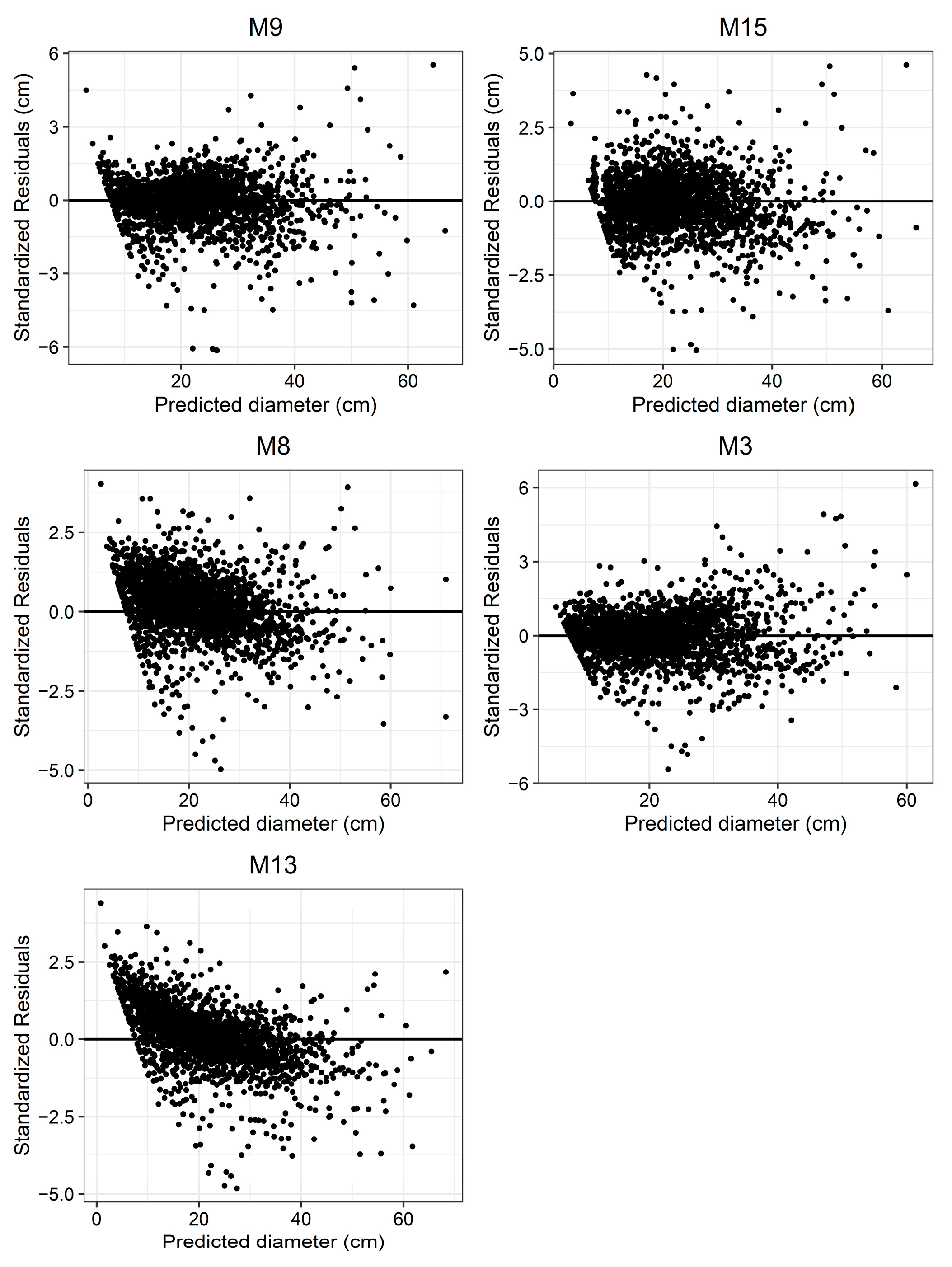
3.2. Residual Diagnostic

Residual diagnostics were carried out after mixed effects modes with the CAR1 and power variance functions (Figure 3). To understand the model bias and potential outliners in predicting upper stem diameters, we plotted standardized residuals against predicted diameters. The five selected models showed a wider spread of residuals for larger diameters, indicating reduced precision in predicting larger values.

The prediction accuracies of the selected models are further examined by dividing the model errors into ten relative height diameter class sizes of 0.1 intervals (inclusive for the lower bound and exclusive for the upper bound; both bounds are inclusive for the last interval class). The variability of the prediction errors within each class is illustrated in Figure 4. M9 showed the least bias and performed better for all relative height classes (except for the last height class, (0.9, 1]). Model M15 showed a negative bias at the bottom and a positive bias at the top height indicating overprediction at the butt and underprediction at the top of the trees. However, M8 and M13 consistently underestimated the upper stem diameters.

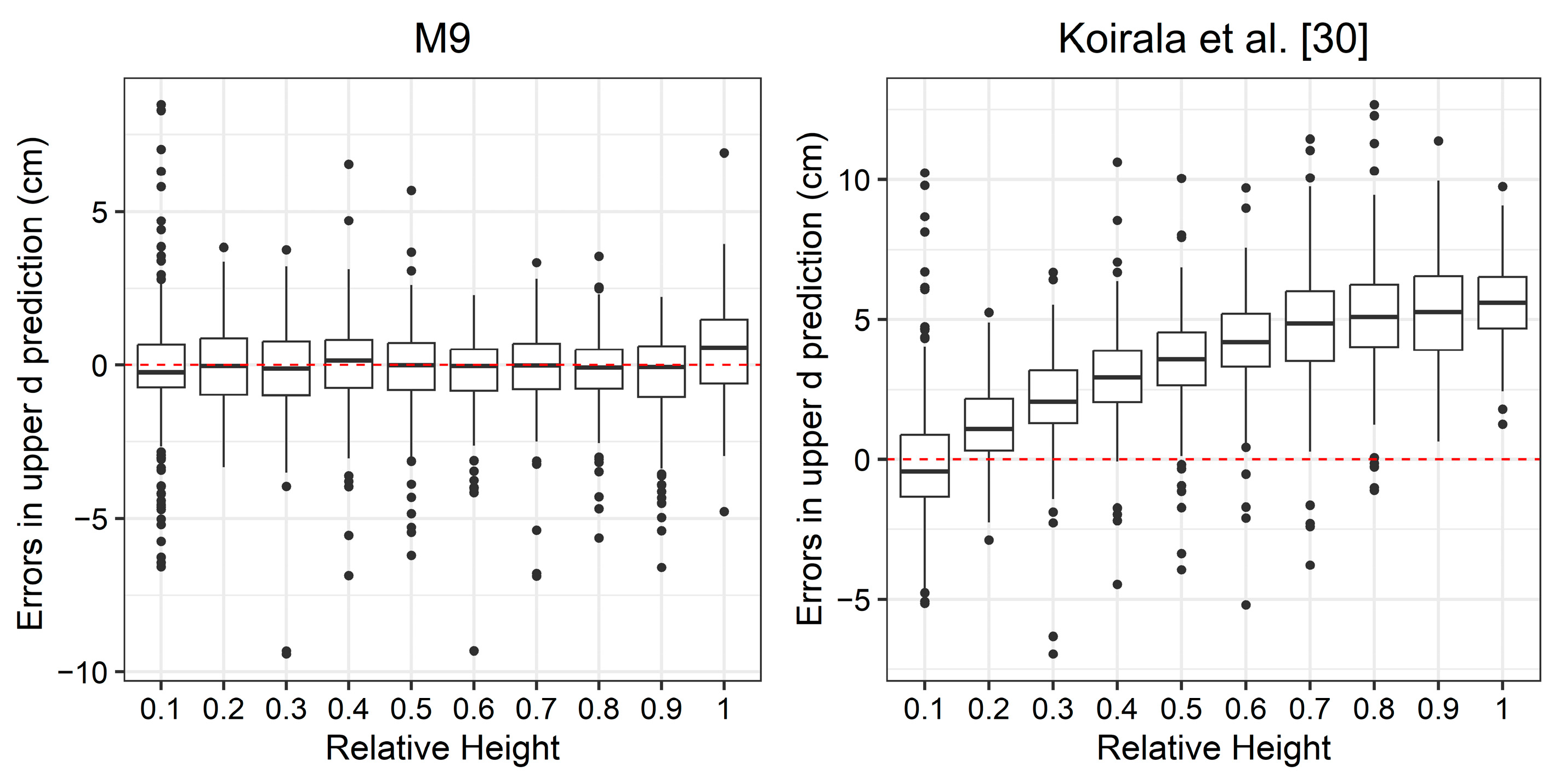
3.3. Model Comparison

Comparing the models M3, M8, M9, M13, and M15 in fit statistics, validation statistics, and residual diagnostics, M9 was selected as the best performer. M9 was also compared with previously published models (M13) (Koirala et al. [30]; hereafter referred to as the Koirala model) based on data sets from the same plantation management regimes in the same region. We used the parameters reported to understand the distribution of residuals between relative height classes (Figure 5). The published study resulted in underprediction across relative height classes except for the first class ((0, 0.1]).

4. Discussion

An accurate estimate of tree taper is important as it is often used in forest inventories to estimate the volume [74,75]. Taper functions offer flexibility and accuracy in volume estimation over volume equations and volume tables [26]. The taper in a tree varies from species to species and is affected by the density, age, and location of a stand [15,20]. To account for this variability, it is necessary to develop/update taper functions for individual tree species and updating the model forms across regions is essential [15,20]. In this study, we examined the 15 available taper equations using data from the planted Teak forests to provide improved taper equations and parameter estimates for the Teak species. We selected the best-performing taper equations from previous studies and different model forms to provide diversity in candidate models. The 15 taper equations were initially examined by 10-fold cross-validation, and five models were selected for further improvements. Under 10-fold cross-validation, the model test and validation statistics were almost similar, reflecting the model robustness in explaining the variability for seen and unseen data.

Among the various model forms selected, the trigonometric variable exponent model (M15) performed better, followed by the variable exponent model (M9) under fixed effects modeling. The trigonometric variable exponent model was originally developed for Eucalyptus species in Australia [56]. We modified this equation by removing the one insignificant term and fitting it for the Teak species. As Teak plantations in the Sagarnath development project co-established with Eucalyptus, it may also be useful in developing taper equations for Eucalyptus. There are limited studies that compare trigonometric variable exponents with other taper forms. Rojo et al. [8] selected five taper functions, including trigonometric variable exponent models, as candidate models (and four different models) out of 31 taper equations for Maritime pine stands. Li and Weiskittel [5] fitted and compared ten widely adopted models, including trigonometric variable exponent equations, to estimate the stem taper for the primary conifer species of the North American Acadian Region. They found that the Bi [56] variable exponent trigonometric equations (M15) and Kozak [4] (M10) equations performed better for red spruce [Picea rubens Sarg.], and white pine [Pinus strobus L.]. Similarly, Poudel et al. [36] also used five taper equations selected by Rojo et al. [8] to evaluate the tree taper of Douglas fir and Western hemlock trees. Both studies found that the Kozak [4] variable exponent equations performed better than the trigonometric variable exponent equations. This could be because the Kozak [4] models were applied to coniferous trees (pine and fir), which have stem forms different from those of hardwood species as in this study. However, planted Teak taper studies mainly used Kozak [4] and Goodwin [48] taper equations to estimate stem tapering without considering other model forms (e.g., [28,49,50]).

As variable exponent models offer flexibility for model shape, they can perform better over simple and segmented polynomials, as in the case of this study [8,9,36,76]. We applied mixed-effects modeling to the top five best performing models to enhance the performance of variable exponent models. The Sharma and Zhang model (M9) demonstrated significant improvement in the mixed modeling framework, achieving better accuracy compared to bi-trigonometric equations (M15). These findings are consistent with previous studies in Nepal, which estimated the upper stem diameter of hardwood and softwood species. Ulak et al. [10] compared seventeen taper equations for tropical hardwood species [Sorea robusta C.F. Gaertn] in Nepal and selected Sharma and Zhang [63] (M9) as models compared to simple and segmented polynomials. Similarly, Saud et al. [11] found that the variable exponent taper function developed by Sharma and Zhang [63] performed better in 13 different taper equations (including segmented polynomials) for natural Chir pine [Pinus roxburghii C. Sargent] species in Nepal. Koirala et al. [30] compared five taper equations to estimate the upper stem diameter of the Teak plantation forest and found that the Graćia [53] (M13) taper functions (derived from dynamic taper functions) as a better predictive model over other variable exponent and segmented polynomials. However, they did not include the variety of models we used in this study while selecting the five best-performing models. This indicates that several candidate models of varying model forms should be selected when selecting the best-performing taper equations.

The Graćia [53] (M13) taper function selected by Koirala et al. [30] to estimate the upper stem diameter of plantation Teak was one of the candidate models considered in our study. This model consistently underestimated the upper stem diameter after the 5th relative height class (Figure 5). Because our study shares a study area with the Koirala et al. [30] study, we compared the performance of the Koirala model with our data set. The best model reported by Koirala et al. [30] predicted the upper diameters at increasing rates from the bottom to the top of the trees. The reason behind the consistent underprediction by the Koirala model could be attributed to the sample size (n = 45 at 3 m intervals) compared to our study (n = 100 at 1 m intervals). Future studies should compare the results of this study for a better prediction of the tree taper in Teak species.

The mixed effects model structure incorporated continuous first-order autocorrelation (CAR1) and the power variance structure improved the goodness of fit (fit statistics) by better explaining the residual patterns of the models. Our result from mixed-effects modeling is in agreement with previous studies (e.g., [11,22,24,36]) who found significant improvements in taper model performance by using a mixed-effects modeling approach with autocorrelations and variance structures. Some studies suggested that more parameters random effects could improve the model performance and address autocorrelation without incorporating the autocorrelation structure [23,77]. However, there is always a trade-off among the number of random-effects coefficients, the complexity of the error covariate structures, and the availability of destructively sampled data [24,35]. Owing to our small sample (n = 100), we only fitted the model with single random-effects parameters with autocorrelations and variance structures. Generally, the coefficient of fixed effects parts in mixed effect modeling are used for model prediction [24,41]. Although mixed effects models tend to offer improved accuracy, they are often not considered practical for obtaining pre-information in large-scale forestry applications [78,79]. Parsimonious and simple models typically have great practical utility. Therefore, identifying an effective and widely used parsimonious model is often considered the ideal scenario in practical forestry.

The CAR1 structures incorporated into mixed models have effectively addressed the inherent autocorrelations among the residuals. This result is comparable to other taper studies [11,36,76,80]. However, studies [8,9,30] found that the CAR2 model was effective as they only used fixed effects modeling. This discrepancy in result may be partly due to the fact that the random effect structure may have addressed some degree of autocorrelation under the mixed effect modeling framework [22,23,24,81] and the CAR1 structures might have further improved inherent autocorrelation. Some models, such as the trigonometric exponential variable (M15), showed much lower autocorrelations, comparable to Rojo et al. [8]. The power variance function of the height sections substantially improved the distribution of the residuals, thereby eliminating any apparent trend and stabilizing the nonhomogeneous variance of the models [29,36,40,80]. Addressing autocorrelation and non-homogeneous structures in modeling does not necessarily enhance predictive ability [24,64]. However, it prevents underestimating the parameter covariance matrix and improves the interpretation of the model’s statistical properties [81]. The model testing statistics obtained with and without autocorrelation and variance structures were also similar in this study (Table 5).

In addition to mixed effect modeling, the performance of the taper equations can be further improved by incorporating crown variables and stand density [5,82]. Other improvements may include using the diameter of the inside bark instead of diameter outside bark [52,63], avoiding trees with more enormous buttresses and deformed trees [83]. Due to logistics and time constraints, we could not obtain the auxiliary data mentioned here during the sampling process. Future taper equations may consider using eucalyptus and Teak measurements and stand and crown variables to further enhance and improve these taper models. Moreover, these taper equations provide valuable information to estimate the volume of Teak trees in any plantation section for Teak trees in the study area region.

5. Conclusions

Existing taper equations for Teak, a broadleaved species, have had limited use in the plantation forests of Nepal and South Asia. Evaluating 15 taper equations and comparing the best-performing models with a published model, we showed that the mixed effects model that includes power variance error structure and continuous first-order autocorrelation improved the fit statistics of taper equations. The Sharma and Zhang [63] model was identified as the best equation for estimating upper stem diameters regarding fit and validation statistics and logical behavior. We encourage future studies to develop and test simple to complex taper models with more data, preferably at shorter intervals, for Teak in the Sagarnath plantation of Nepal. We also recommend using multiple equations for model improvement, rather than focusing on a single equation during model selection. Our model behaved well and now allows for a quick estimate of the volume and upper diameters of Teak for forest management, planning, and research in the Sagarnath plantation region of Nepal.

References

1. Burkhart, H.E.; Tomé, M. Modeling Forest Trees and Stands; Springer: Berlin/Heidelberg, Germany, 2012; Volume 457. [Google Scholar]
2. Parresol, B.R. Assessing Tree and Stand Biomass: A Review with Examples and Critical Comparisons. For. Sci. 1999, 45, 573–593. [Google Scholar] [CrossRef]
3. Westfall, J.A.; Coulston, J.W.; Gray, A.N.; Shaw, J.D.; Radtke, P.J.; Walker, D.M.; Weiskittel, A.R.; MacFarlane, D.W.; Affleck, D.L.R.; Zhao, D. A National-Scale Tree Volume, Biomass, and Carbon Modeling System for the United States; Gen. Tech. Rep. WO-104; US Department of Agriculture, Forest Service: Washington, DC, USA, 2024; Volume 104. [Google Scholar]
4. Kozak, A. My Last Words on Taper Equations. For. Chron. 2004, 80, 507–515. [Google Scholar] [CrossRef]
5. Li, R.; Weiskittel, A.R. Comparison of Model Forms for Estimating Stem Taper and Volume in the Primary Conifer Species of the North American Acadian Region (Comparaison de Formules Modèles Pour Estimer La Décroissance de La Tige et Le Volume Des Principales Espèces de Conifères Dan). Ann. For. Sci. 2010, 67, 302. [Google Scholar]
6. Fonweban, J.; Gardiner, B.; Macdonald, E.; Auty, D. Taper Functions for Scots Pine (Pinus sylvestris L.) and Sitka Spruce (Picea Sitchensis (Bong.) Carr.) in Northern Britain. Forestry 2011, 84, 49–60. [Google Scholar] [CrossRef]
7. Dahlen, J.; Auty, D.; Eberhardt, T.L. Models for Predicting Specific Gravity and Ring Width for Loblolly Pine from Intensively Managed Plantations, and Implications for Wood Utilization. Forests 2018, 9, 292. [Google Scholar] [CrossRef]
8. Rojo, A.; Perales, X.; Sánchez-Rodríguez, F.; Álvarez-González, J.G.; von Gadow, K. Stem Taper Functions for Maritime Pine (Pinus pinaster Ait.) in Galicia (Northwestern Spain). Eur. J. For. Res. 2005, 124, 177–186. [Google Scholar] [CrossRef]
9. Diéguez-Aranda, U.; Castedo-Dorado, F.; Álvarez-González, J.G.; Rojo, A. Compatible Taper Function for Scots Pine Plantations in Northwestern Spain. Can. J. For. Res. 2006, 36, 1190–1205. [Google Scholar] [CrossRef]
10. Ulak, S.; Ghimire, K.; Gautam, R.; Bhandari, S.K.; Poudel, K.P.; Timilsina, Y.P.; Pradhan, D.; Subedi, T. Predicting the Upper Stem Diameters and Volume of a Tropical Dominant Tree Species. J. For. Res. 2022, 33, 1725–1737. [Google Scholar] [CrossRef]
11. Saud, P.; Chapagain, T.R.; Bhandari, S.K.; Moser, W.K. Taper Functions to Predict the Upper Stem Diameter of Chir Pine (Pinus roxburghii) in the Mid-Hills of Nepal. Trees For. People 2024, 17, 100627. [Google Scholar] [CrossRef]
12. Tasissa, G.; Burkhart, H.E. An Application of Mixed Effects Analysis to Modeling Thinning Effects on Stem Profile of Loblolly Pine. For. Ecol. Manag. 1998, 103, 87–101. [Google Scholar] [CrossRef]
13. Sabatia, C.O.; Burkhart, H.E. Segmented Taper Equation to New Trees. For. Sci. 2015, 61, 411–423. [Google Scholar]
14. Max, T.; Burkhart, H.E. Segmented Polynomial Regression Applied to Taper Equations. For. Sci. 1976, 22, 283–289. [Google Scholar]
15. McTague, J.P.; Weiskittel, A. Evolution, History, and Use of Stem Taper Equations: A Review of Their Development, Application, and Implementation. Can. J. For. Res. 2021, 51, 210–235. [Google Scholar] [CrossRef]
16. Zapata-Cuartas, M.; Bullock, B.P.; Montes, C.R. A Taper Equation for Loblolly Pine Using Penalized Spline Regression. For. Sci. 2021, 67, 1–13. [Google Scholar] [CrossRef]
17. Scolforo, H.F.; McTague, J.P.; Raimundo, M.R.; Weiskittel, A.; Carrero, O.; Scolforo, J.R.S. Comparison of Taper Functions Applied to Eucalypts of Varying Genetics in Brazil: Application and Evaluation of the Penalized Mixed Spline Approach. Can. J. For. Res. 2018, 48, 568–580. [Google Scholar] [CrossRef]
18. Nunes, M.H.; Görgens, E.B. Artificial Intelligence Procedures for Tree Taper Estimation within a Complex Vegetation Mosaic in Brazil. PLoS ONE 2016, 11, 1–16. [Google Scholar] [CrossRef]
19. Yang, S.I.; Burkhart, H.E. Robustness of Parametric and Nonparametric Fitting Procedures of Tree-Stem Taper with Alternative Definitions for Validation Data. J. For. 2020, 118, 576–583. [Google Scholar] [CrossRef]
20. Salekin, S.; Catalán, C.H.; Boczniewicz, D.; Phiri, D.; Morgenroth, J.; Meason, D.F.; Mason, E.G. Global Tree Taper Modelling: A Review of Applications, Methods, Functions, and Their Parameters. Forests 2021, 12, 913. [Google Scholar] [CrossRef]
21. Yang, S.I.; Burkhart, H.E.; Seki, M. Evaluating Semi- and Nonparametric Regression Algorithms in Quantifying Stem Taper and Volume with Alternative Test Data Selection Strategies. Forestry 2023, 96, 465–480. [Google Scholar] [CrossRef]
22. Trincado, G.; Burkhart, H.E. A Generalized Approach for Modeling and Localizing Stem Profile Curves. For. Sci. 2006, 52, 670–682. [Google Scholar] [CrossRef]
23. Yang, Y.; Huang, S.; Trincado, G.; Meng, S.X. Nonlinear Mixed-Effects Modeling of Variable-Exponent Taper Equations for Lodgepole Pine in Alberta, Canada. Eur. J. For. Res. 2009, 128, 415–429. [Google Scholar] [CrossRef]
24. Gómez-García, E.; Crecente-Campo, F.; Diéguez-Aranda, U. Selection of Mixed-Effects Parameters in a Variable-Exponent Taper Equation for Birch Trees in Northwestern Spain. Ann. For. Sci. 2013, 70, 707–715. [Google Scholar] [CrossRef]
25. Berger, A.; Gschwantner, T.; McRoberts, R.E.; Schadauer, K. Effects of Measurement Errors on Individual Tree Stem Volume Estimates for the Austrian National Forest Inventory. For. Sci. 2014, 60, 14–24. [Google Scholar] [CrossRef]
26. Zhao, D.; Lynch, T.B.; Westfall, J.; Coulston, J.; Kane, M.; Adams, D.E. Compatibility, Development, and Estimation of Taper and Volume Equation Systems. For. Sci. 2019, 65, 1–13. [Google Scholar] [CrossRef]
27. He, P.; Hussain, A.; Khurram Shahzad, M.; Jiang, L.; Li, F. Evaluation of Four Regression Techniques for Stem Taper Modeling of Dahurian Larch (Larix gmelinii) in Northeastern China. For. Ecol. Manag. 2021, 494, 119336. [Google Scholar] [CrossRef]
28. Noda, I.; Himmapan, W.; Furuya, N.; Hitsuma, G. Taper Equations for Evaluating Private Plantation Teak (Tectona grandis) in Thailand. Jpn. Agric. Res. Q. 2023, 57, 329–343. [Google Scholar] [CrossRef]
29. Poudel, K.P.; Özçelik, R.; Yavuz, H. Differences in Stem Taper of Black Alder (Alnus Glutinosa Subsp. Barbata) by Origin. Can. J. For. Res. 2020, 50, 581–588. [Google Scholar] [CrossRef]
30. Koirala, A.; Montes, C.R.; Bullock, B.P.; Wagle, B.H. Developing Taper Equations for Planted Teak (Tectona grandis L.f.) Trees of Central Lowland Nepal. Trees For. People 2021, 5, 100103. [Google Scholar] [CrossRef]
31. Lumumba, V.W.; Kiprotich, D.; Makena, N.G.; Kavita, M.D.; Mpaine, M.L. Comparative Analysis of Cross-Validation Techniques: LOOCV, K-Folds Cross-Validation, and Repeated K-Folds Cross-Validation in Machine Learning Models. Am. J. Theor. Appl. Stat. 2024, 13, 127–137. [Google Scholar] [CrossRef]
32. Gareth, J.; Daniela, W.; Trevor, H.; Robert, T. An Introduction to Statistical Learning: With Applications in R; Spinger: Berlin/Heidelberg, Germany, 2013. [Google Scholar]
33. Adhikari, A.; Montes, C.R.; Peduzzi, A. A Comparison of Modeling Methods for Predicting Forest Attributes Using Lidar Metrics. Remote. Sens. 2023, 15, 1284. [Google Scholar] [CrossRef]
34. Bennett, F.; Swindel, B. Taper Curves for Planted Slash Pine. USDA For. Serv. Res. Note Southeast. For. Exp. Stn. 1972, 4, ref.5. [Google Scholar]
35. Pinheiro, J.C.; Bates, D.M. Fitting Nonlinear Mixed-Effects Models. In Mixed-Effects Models in S and S-PLUS; Springer: New York, NY, USA, 2000; pp. 337–421. [Google Scholar]
36. Poudel, K.P.; Temesgen, H.; Gray, A.N. Estimating Upper Stem Diameters and Volume of Douglas-Fir and Western Hemlock Trees in the Pacific Northwest. For. Ecosyst. 2018, 5, 16. [Google Scholar] [CrossRef]
37. Littell, R.; Stroup, W.; Wolfinger, R.; Schabenberger, O.; Milliken, G.A. SAS for Mixed Models, 2nd ed.; SAS Institute Inc.: Cary, NC, USA, 2006; p. 814. [Google Scholar]
38. Davidian, M.; Giltinan, D.M. Nonlinear Models for Repeated Measurement Data; Routledge: New York, NY, USA, 2017; ISBN 9780203745502. [Google Scholar]
39. Lindstrom, M.J.; Bates, D.M. Nonlinear Mixed Effects Models for Repeated Measures Data. Biometrics 1990, 46, 673–687. [Google Scholar] [CrossRef] [PubMed]
40. Li, R.; Weiskittel, A.; Dick, A.R.; Kershaw, J.A.; Seymour, R.S. Regional Stem Taper Equations for Eleven Conifer Species in the Acadian Region of North America: Development and Assessment. North. J. Appl. For. 2012, 29, 5–14. [Google Scholar] [CrossRef]
41. de-Miguel, S.; Mehtätalo, L.; Shater, Z.; Kraid, B.; Pukkala, T. Evaluating Marginal and Conditional Predictions of Taper Models in the Absence of Calibration Data. Can. J. For. Res. 2012, 42, 1383–1394. [Google Scholar] [CrossRef]
42. Tewari, D.N. A Monograph on Teak (Tectona grandis Linn. f.); International Book Distributors: Dehra Dun, India, 1992; Volume 479. [Google Scholar]
43. Kollert, W.; Kleine, M. The Global Teak Study. Analysis, Evaluation and Future Potential of Teak Resources; International Union of Forest Research Organizations: Vienna, Austria, 2017. [Google Scholar]
44. Moya, R.; Bond, B.; Quesada, H. A Review of Heartwood Properties of Tectona Grandis Trees from Fast-Growth Plantations. Wood Sci. Technol. 2014, 48, 411–433. [Google Scholar] [CrossRef]
45. ADB. Project Performance Audit Report Sagarnath Forestry Development Project in Nepal; Asian Development Bank: Kathmandu, Nepal, 1987. [Google Scholar]
46. Adu-Bredu, S.; Bi, A.F.T.; Bouillet, J.P.; Mé, M.K.; Kyei, S.Y.; Saint-André, L. An Explicit Stem Profile Model for Forked and Un-Forked Teak (Tectona grandis) Trees in West Africa. For. Ecol. Manag. 2008, 255, 2189–2203. [Google Scholar] [CrossRef]
47. Shuaibu, R. Developing Stem Taper Equation for Tectona grandis (Teak) Plantation in Agudu Forest Reserve, Nasarawa State, Nigeria. J. Sci. Technol. 2016, 5, 199–206. [Google Scholar]
48. Goodwin, A.N. A Cubic Tree Taper Model. Aust. For. 2009, 72, 87–98. [Google Scholar] [CrossRef]
49. Warner, A.J.; Jamroenprucksa, M.; Puangchit, L. Development and Evaluation of Teak (Tectona grandis L.f.) Taper Equations in Northern Thailand. Agric. Nat. Resour. 2016, 50, 362–367. [Google Scholar] [CrossRef]
50. Choochuen, T.; Suksavate, W.; Meunpong, P. Development of a Taper Equation for Teak (Tectona grandis l.f.) Growing in Western Thailand. Environ. Nat. Resour. J. 2021, 19, 176–185. [Google Scholar] [CrossRef]
51. Kozak, A.; Munro, D.D.; Smith, J.H.G. Taper Functions and Their Application in Forest Inventory. For. Chron. 1969, 45, 278–283. [Google Scholar] [CrossRef]
52. Sharma, M.; Parton, J. Spruce Plantations Using Dimensional Analysis. For. Sci. 2009, 55, 268–282. [Google Scholar]
53. García, O. Dynamic Modelling of Tree Form. Math. Comput. For. Nat. Resour. Sci. 2015, 7, 9–15. [Google Scholar]
54. FRA/DFRS. Terai Forests of Nepal (2010–2012), Forest Resource Assessment Nepal Project/Department of Forest Research and Survey; FRA/DFRS: Babarmahal, Kathmandu, Nepal, 2014. [Google Scholar]
55. ADB. Re-Evaluation of the Sagarnath Forestry Development Project in Nepal; Asian Development Bank: Kathmandu, Nepal, 1993. [Google Scholar]
56. Bi, H. Trigonometric Variable-Form Taper Equations for Australian Eucalypts. For. Sci. 2000, 46, 397–409. [Google Scholar] [CrossRef]
57. Cervera, J.M. El Área Basimétrica Reducida, El Volumen Reducido y El Perfil. Montes 1973, 174, 415–418. [Google Scholar]
58. Amidon, E.L. A General Taper Functional Form to Predict Bole Volume for Five Mixed-Conifer Species in California. For. Sci. 1984, 30, 166–171. [Google Scholar]
59. Oderwald, R.G.; Rayamajhi, J.N. Biomass Inventory with Tree Taper Equations. Bioresour. Technol. 1991, 36, 235–239. [Google Scholar] [CrossRef]
60. Ormerod, D.W. A Simple Bole Model. For. Chron. 1973, 49, 136–138. [Google Scholar] [CrossRef]
61. Clutter, J.L. Development of Taper Functions from Variable-Top Merchantable Volume Equations. For. Sci. 1980, 26, 117–120. [Google Scholar] [CrossRef]
62. Sharma, M.; Oderwald, R.G. Dimensionally Compatible Volume and Taper Equations. Can. J. For. Res. 2001, 31, 797–803. [Google Scholar] [CrossRef]
63. Sharma, M.; Zhang, S.Y. Variable-Exponent Taper Equations for Jack Pine, Black Spruce, and Balsam Fir in Eastern Canada. For. Ecol. Manag. 2004, 198, 39–53. [Google Scholar] [CrossRef]
64. Arias-Rodil, M.; Diéguez-Aranda, U.; Puerta, F.R.; López-Sánchez, C.A.; Líbano, E.C.; Obregón, A.C.; Castedo-Dorado, F. Modelling and Localizing a Stem Taper Function for Pinus Radiata in Spain. Can. J. For. Res. 2015, 45, 647–658. [Google Scholar] [CrossRef]
65. Poudel, K.P.; Cao, Q.V. Evaluation of Methods to Predict Weibull Parameters for Characterizing Diameter Distributions. For. Sci. 2013, 59, 243–252. [Google Scholar] [CrossRef]
66. Subedi, M.R.; Oli, B.N.; Shrestha, S.; Chhin, S. Height-Diameter Modeling of Cinnamomum Tamala Grown in Natural Forest in Mid-Hill of Nepal. Int. J. For. Res. 2018, 2018, 1–11. [Google Scholar] [CrossRef]
67. Raut, S.; Dahlen, J.; Bullock, B.; Montes, C.; Dickens, D. Models to Predict Whole-Disk Specific Gravity and Moisture Content in Planted Longleaf Pine from Cutover and Old Field Sites. Can. J. For. Res. 2022, 52, 137–147. [Google Scholar] [CrossRef]
68. Aryal, S.; Gaire, N.P.; Pokhrel, N.R.; Rana, P.; Sharma, B.; Kharal, D.K.; Poudel, B.S.; Dyola, N.; Fan, Z.X.; Grießinger, J.; et al. Spring Season in Western Nepal Himalaya Is Not yet Warming: A 400-Year Temperature Reconstruction Based on Tree-Ringwidths of Himalayan Hemlock (Tsuga dumosa). Atmosphere 2020, 11, 132. [Google Scholar] [CrossRef]
69. Dahlen, J.; Auty, D.; Eberhardt, T.L.; Schimleck, L.; Pokhrel, N.R. Determination of Ring-Level Dynamic Modulus of Elasticity in Loblolly Pine from Measurements of Ultrasonic Velocity and Specific Gravity. Forestry 2023, 96, 588–604. [Google Scholar] [CrossRef]
70. R Core Team. R: A Language and Environment for Statistical Computing; R Foundation for Statistical Computing: Vienna, Austria, 2024. [Google Scholar]
71. RStudio Team. R Studio: Integrated Development for R; RStudio: Vienna, Austria, 2024. [Google Scholar]
72. Pinheiro, J.; Bates, D.; DebRoy, S.; Sarkar, D.; Heisterkamp, S.; Van Willigen, B.; Maintainer, R. Package ‘Nlme’. Linear Nonlinear Mix. Eff. Models Version 2017, 3, 274. [Google Scholar]
73. Wickham, H.; Averick, M.; Bryan, J.; Chang, W.; D’Agostino McGowan, L.; François, R.; Grolemund, G.; Hayes, A.; Henry, L.; Hester, J.; et al. Welcome to the Tidyverse. J. Open Source Softw. 2019, 4, 1686. [Google Scholar] [CrossRef]
74. Weiskittel, A.R.; Hann, D.W.; Kershaw, J.A., Jr.; Vanclay, J.K. Forest Growth and Yield Modeling; John Wiley & Sons, Ltd.: Milton, QLD, Australia, 2011; ISBN 0470665009. [Google Scholar]
75. Mehtatalo, L.; Lappi, J. Biometry for Forestry and Environmental Data: With Examples in R; Chapman and Hall/CRC: Boca Raton, FL, USA, 2020; ISBN 0429173466. [Google Scholar]
76. Weiskittel, A.R.; Li, R. Development of Regional Taper and Volume Equations: Hardwood Species. In Cooperative Forestry Research Unit: 2011 Annual Report; University of Maine: Orono, ME, USA, 2012; Volume i, pp. 76–83. [Google Scholar]
77. Yang, Y.; Huang, S.; Meng, S.X. Development of a Tree-Specific Stem Profile Model for White Spruce: A Nonlinear Mixed Model Approach with a Generalized Covariance Structure. Forestry 2009, 82, 541–555. [Google Scholar] [CrossRef]
78. Subedi, M.R.; Zhao, D.; Dwivedi, P.; Costanzo, B.E.; Martin, J.A. Site Index Models for Loblolly Pine Forests in the Southern United States Developed with Forest Inventory and Analysis Data. For. Sci. 2023, 69, 597–609. [Google Scholar] [CrossRef]
79. Wang, M.; Montes, C.R.; Bullock, B.P.; Zhao, D. An Empirical Examination of Dominant Height Projection Accuracy Using Difference Equation Models. For. Sci. 2020, 66, 267–274. [Google Scholar] [CrossRef]
80. dos Santos, M.L.; Miguel, E.P.; Biali, L.J.; de Souza, H.J.; dos Santos, C.R.C.; Matricardi, E.A.T. The Effect of Age on the Evolution of the Stem Profile and Heartwood Proportion of Teak Clonal Trees in the Brazilian Amazon. Forests 2023, 14, 1962. [Google Scholar] [CrossRef]
81. Garber, S.M.; Maguire, D.A. Modeling Stem Taper of Three Central Oregon Species Using Nonlinear Mixed Effects Models and Autoregressive Error Structures. For. Ecol. Manag. 2003, 179, 507–522. [Google Scholar] [CrossRef]
82. Leites, L.P.; Robinson, A.P. Improving Taper Equations of Loblolly Pine with Crown Dimensions in a Mixed-Effects Modeling Framework. For. Sci. 2004, 50, 204–212. [Google Scholar] [CrossRef]
83. Warner, A.J.; Jamroenprucksa, M.; Puangchit, L. Buttressing Impact on Diameter Estimation in Plantation Teak (Tectona grandis L.f.) Sample Trees in Northern Thailand. Agric. Nat. Resour. 2017, 51, 520–525. [Google Scholar] [CrossRef]
Figure 1. Location map of the study area and sampling sites.
Forests 16 00077 g001
Figure 2. Scatter plot of total height against diameter at breast height (d) (left) and relative diameter (d/D) against relative height (h/H) (right).
Forests 16 00077 g002
Figure 3. Standardized residuals versus the predicted upper stem diameter of the five selected taper models.
Forests 16 00077 g003
Figure 4. Box plots showing the variations in the model errors in predictive upper stem diameter at the 0.1 relative height interval class for five selected taper equations.
Forests 16 00077 g004
Figure 5. Comparison of prediction errors in stem diameter at upper heights—Koirala et al. (2021) [30]—versus this study using the current data set.
Forests 16 00077 g005