Single-Species Leaf Detection against Complex Backgrounds with YOLOv5s

Abstract

Accurate and rapid localization and identification of tree leaves are of significant importance for urban forest planning and environmental protection. Existing object detection neural networks are complex and often large, which hinders their deployment on mobile devices and compromises their efficiency in detecting plant leaves, especially against complex backgrounds. To address this issue, we collected eight common types of tree leaves against complex urban backgrounds to create a single-species leaf dataset. Each image in this dataset contains only one type of tree but may include multiple leaves. These leaves share similar shapes and textures and resemble various real-world background colors, making them difficult to distinguish and accurately identify, thereby posing challenges to model precision in localization and recognition. We propose a lightweight single-species leaf detection model, SinL-YOLOv5, which is only 15.7 MB. First, we integrated an SE module into the backbone to adaptively adjust the channel weights of feature maps, enhancing the expression of critical features such as the contours and textures of the leaves. Then, we developed an adaptive weighted bi-directional feature pyramid network, SE-BiFPN, utilizing the SE module within the backbone. This approach enhances the information transfer capabilities between the deep semantic features and shallow contour texture features of the network, thereby accelerating detection speed and improving detection accuracy. Finally, to enhance model stability during learning, we introduced an angle cost-based bounding box regression loss function (SIoU), which integrates directional information between ground-truth boxes and predicted boxes. This allows for more effective learning of the positioning and size of leaf edges and enhances the model’s accuracy in detecting leaf locations. We validated the improved model on the single-species leaf dataset. The results showed that compared to YOLOv5s, SinL-YOLOv5 exhibited a notable performance improvement. Specifically, SinL-YOLOv5 achieved an increase of nearly 4.7 percentage points in the [email protected] and processed an additional 20 frames per second. These enhancements significantly enhanced both the accuracy and speed of localization and recognition. With this improved model, we achieved accurate and rapid detection of eight common types of single-species tree leaves against complex urban backgrounds, providing technical support for urban forest surveys, urban forestry planning, and urban environmental conservation.

1. Introduction

The forest system is an important ecosystem on Earth, and it plays an irreplaceable role in the development of the environment, society, and the economy. Trees are the main component of the forest system, and their growth not only produces huge carbon sinks, alleviating the problems caused by carbon emissions, but also prevents wind and sand damage while nourishing soil and water [1]. At the same time, with the rapid development of urbanization in various countries, concepts such as urban forests have emerged. Urban forests refer to trees managed by the city and various stakeholders, growing in public areas and private gardens [2]. Urban forests play an important role in lowering the ambient temperature, mitigating the urban heat island effect, mitigating climate change, and enhancing the aesthetics of cities [3]. As the level of urban greening continues to rise, the task of leaf cleanup has become increasingly complex and laborious. Leaf litter has seasonal characteristics, requiring repeated sweeping. Relying solely on manual cleanup is not only time-consuming and labor-intensive but also inefficient. In recent years, the development of smart sanitation vehicles equipped with technology to locate leaves has facilitated intelligent leaf cleaning [4]. Therefore, researching intelligent leaf positioning holds significant value for the widespread application of smart sanitation vehicles. In conclusion, accurately locating leaves and identifying tree species are of great importance for urban forest surveys, urban forestry planning, and the maintenance of urban environments.

Plants can be identified using various organs, including leaves, flowers, fruits, and roots. According to recent studies on plants [5], the flowers, fruits, and roots of plants are less suitable for species identification compared to leaves. Due to the fact that the flowers and fruits of the plant only appear during specific seasons, they exist for a relatively brief period of time. Furthermore, roots are situated at a considerable depth within the soil, which makes them difficult to obtain. Compared to other parts of a plant, leaves are the primary organ used for plant identification and classification. Leaves generally grow on the surface of plants and are abundantly present throughout the plant’s lifecycle, making them easily collectible and accessible. Additionally, the shape and structure of leaves are stable and do not change over time. Therefore, leaves are commonly used for classifying and identifying plant species. Plant leaves can typically be described using basic visual features such as color, texture, or shape. Compared to other visual features, the color characteristics of leaves are usually not used alone for plant identification because the leaves of most plant species share common colors, such as green or red. Therefore, existing methods of plant identification typically utilize shape or texture features for recognition. As members of the plant kingdom, trees’ leaves contain species-specific information such as texture, contours, venation, and color. Moreover, the three-dimensional appearance of leaves differs from that of flowers and fruits, with leaves typically having a flat structure [6]. This structure makes leaves easy to collect and preserve and allows for relatively straightforward extraction of complete features from images. Therefore, leaves play a critically important role in the identification of tree species.

Research into tree leaf identification has evolved in two main stages: initially relying on manual identification or feature extraction, and currently utilizing deep learning models to autonomously detect and further identify leaves by extracting their contour and venation features. In the 1990s, the results of Yonekawa [7] and others showed that the characteristic factor of leaf shape played a dominant role in leaf recognition. Researchers used a simple dimensionless shape factor to determine the type of leaf. At the same time, the density, roundness, elongation, shape, and roughness of the leaf were introduced as criteria for the determination of leaf identification. Building on this foundation, more scholars have applied comprehensive information, such as leaf texture and shape features, to leaf identification. At the beginning of the 21st century, Wang et al. [8] integrated pre-segmentation processing and morphological operations into the watershed segmentation algorithm for automatic labeling. They proposed an effective method for leaf image recognition, which utilizes a priori shape information to segment the object contour of the leaf and then extracts the geometry and feature matrix from the segmented binary image to achieve leaf recognition. A method utilizing Support Vector Machine (SVM) to determine the type of leaf was proposed in [9], in which ten feature parameters were selected as the factors to discriminate the leaf species, and the preprocessed image samples were input into the constructed SVM model for training. The experimental data showed that the SVM with a linear kernel function could more accurately determine the leaf species. Between 2015 and 2016, Munisami et al. [10] proposed using the image histogram and multi-dimensional leaf shape features as the basis for discrimination, combined with the K-Nearest Neighbor (KNN) algorithm, to identify more than 30 types of leaf monomers against a white background, achieving high recognition accuracy. In the same period, another proposed method involved combining Gabor filtering and Hu moment invariants to improve the robustness of leaf monomer recognition [11]. Between 2017 and 2018, a model based on a semi-supervised clustering algorithm was used to recognize multiple leaves [12]. Zhang et al. [13] and others proposed combining the Fourier descriptor and the histogram of oriented gradient (HOG) as a feature factor for discriminating tree leaves. Based on this combination, typical correlation analysis was introduced to fuse object features at different scales, which, in turn, improved the ability for leaf recognition. Wang et al. [14] used the KNN algorithm and the covariance matrix algorithm to extract the grayscale texture parameters of tree leaves. In general, traditional leaf-recognition methods primarily focus on leaf monomer images in simple backgrounds, seldom involving realistic, complex backgrounds or the natural habitats of leaves, and there are fewer objects to be recognized in the images. In addition, recognition methods mainly rely on edge extraction, histogram calculation, and SVM application. This makes the recognition process longer and hinders accurate leaf object recognition in real leaf survival environments.

With the rapid development of convolutional neural networks in object recognition, we can autonomously learn the differences between different objects from a large amount of leaf sample data. The computer extracts, processes, and understands the information in the input image, which is then used to detect and recognize objects. As an advanced model structure, convolutional neural networks are able to extract more expressive feature information from images, which greatly improves the performance of modern object recognition systems. Mainstream object recognition networks mainly include SSD [15], the YOLO (You Only Look Once) series [16,17,18,19,20], and the R-CNN series [21,22,23]. As early as the 1980s, the concept of convolutional neural networks was proposed by Lecun [24]. Building on this foundation, the classical framework of convolutional neural networks, LeNet [25], was proposed in the late 1990s. A hierarchical convolutional neural network designed according to the RGB three-channel design of color leaf images was proposed [26]. This network combines the design pattern of LeNet, samples eight network layers for each color channel, and employs SVM and Softmax [27] classifiers to recognize the augmented multiple-leaf images. He et al. [28] proposed a deep residual neural network (Residual Network, ResNet) based on the previously mentioned research. In order to improve the accuracy of recognizing single images of leaves, a recognition method using the HOG operator was proposed based on a convolutional neural network to extract the features of leaves [29]. Xu [30] also proposed fusing the feature maps’ output from networks such as ResNet50, Inception [31], and VGG19 [32] using multiple model-fusion techniques. This method performs global pooling and nonlinear transformation processing on the fused leaf feature maps, ultimately achieving improved recognition performance. Compared with traditional leaf recognition methods, convolutional neural networks can greatly improve recognition accuracy. This is mainly due to the continuous training of the network model with a large number of leaves, which enables it to learn more subtle differences between different types of leaves.

Accurately locating each leaf and correctly identifying its species against complex backgrounds presents a significant challenge in this study. In real and complex environments, leaves that are similar in color to the background, small in size, or overlapping can easily blend into their surroundings, making them difficult to distinguish in images even under suitable lighting or from the right angles. To address these challenges, this study utilizes a dataset composed of images of eight common types of tree leaves collected in urban settings against complex backgrounds. In the dataset, the leaves within each image share similar shape and texture characteristics. Moreover, each image contains only one species of tree but includes multiple leaves, forming a single-species leaf dataset. Additionally, we propose the application of the SinL-YOLOv5 key feature detection model to this dataset for experimental validation, aimed at enhancing the model’s ability to locate and identify tree leaf species within urban environmental backgrounds. The main contributions of this study are as follows:

• To address the issue of feature map loss across different channels during the convolutional pooling process due to varying degrees of importance, we propose a backbone network integrated with an adaptive feature extraction module to enhance the representation capability of key leaf characteristic information;
• An improved feature fusion structure is proposed, which enhances the information transfer capabilities between the model’s deep semantic features and shallow contour texture features. This approach prevents the loss of feature information, accelerates detection speed, and improves the accuracy of object detection;
• A boundary box loss function based on angle cost is introduced, which integrates directional information between ground-truth boxes and predicted boxes, thereby enhancing the accuracy of leaf position detection.

2. Materials and Methods

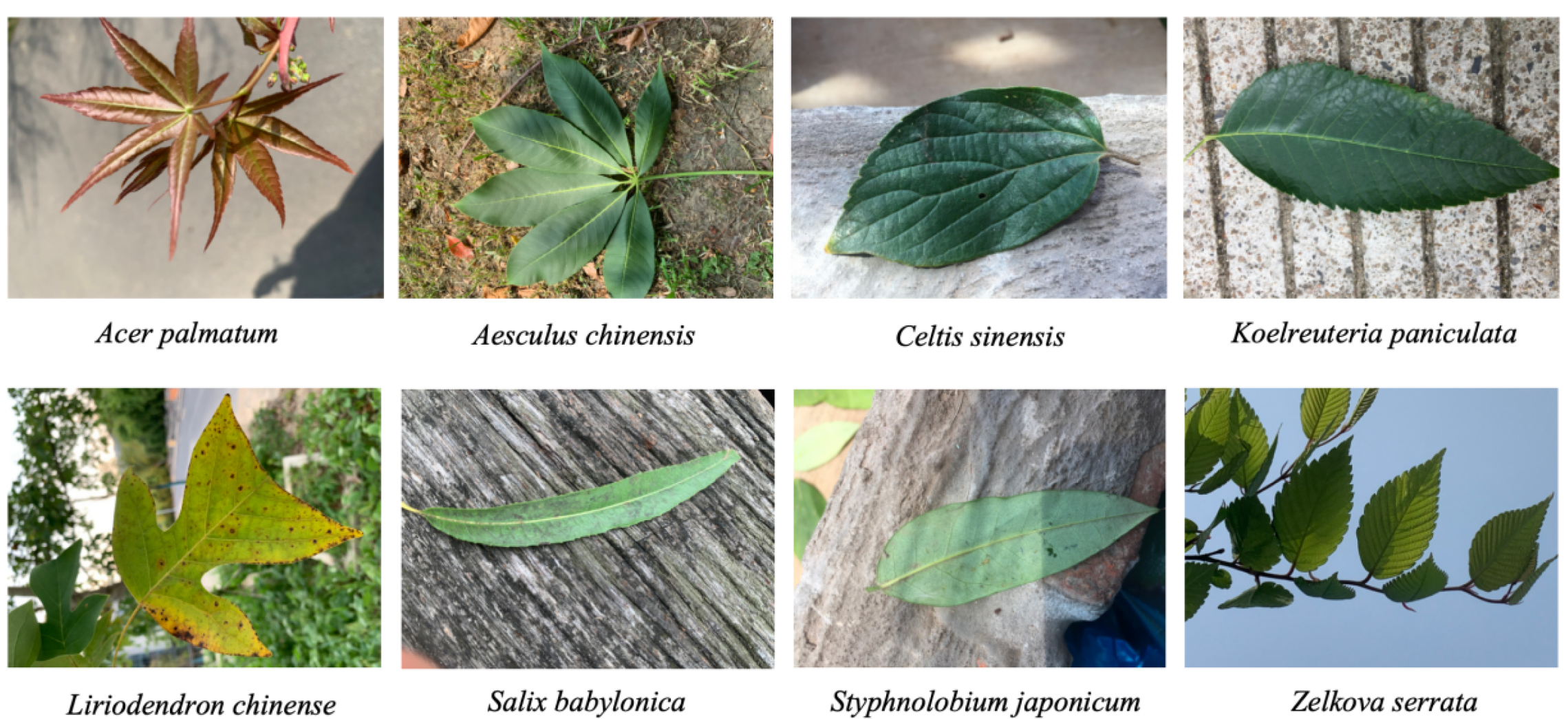
2.1. Datasets

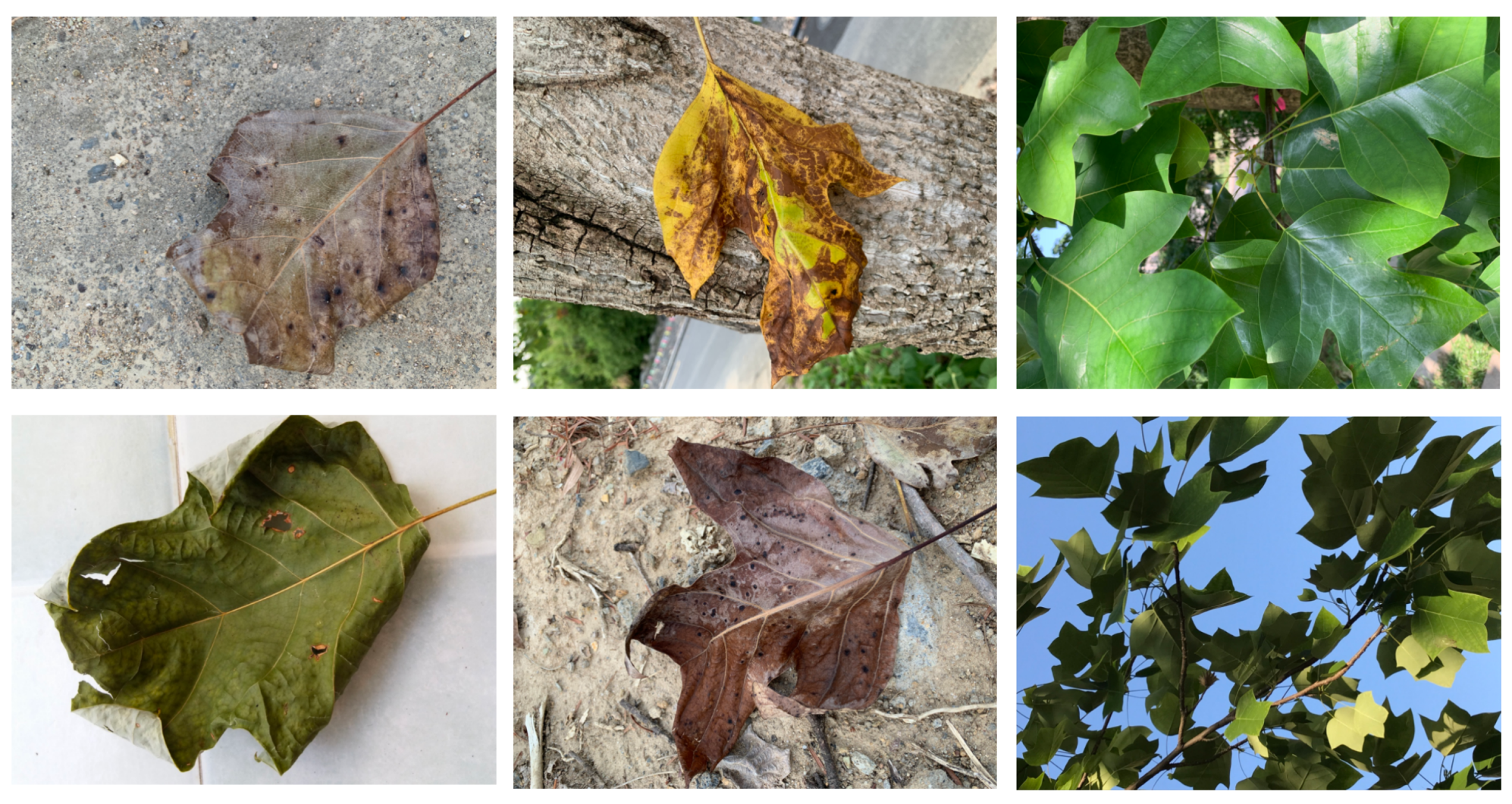
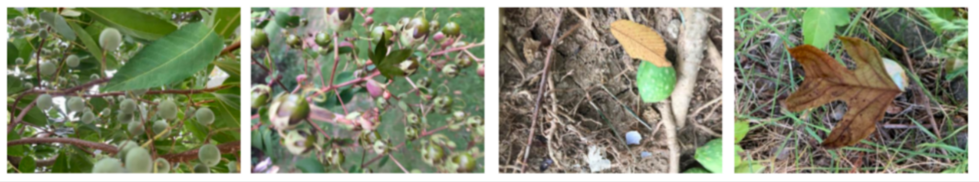
2.1.1. Dataset Acquisition

Due to the ease of collecting and storing tree leaves, which also contain detailed species information, this study chooses tree leaves for identifying tree species. In current leaf identification research, datasets such as Flavia [33], Leafsnap [34], and Swedish [35] are primarily used. Although these datasets feature many species of leaves, the images typically show individual leaves against a uniform (white or black) background, and the number of images per species is relatively low. This scenario makes effective training difficult and does not allow for accurate identification of leaves against complex, real-world backgrounds.

In response to the limitations mentioned, we constructed a leaf image dataset using our own photography and data augmentation methods. The dataset contains images of eight common landscape trees in the cities of Nanjing, Hangzhou, Hefei, and Yangzhou in the Yangtze River Delta region of China as data samples. These include Liriodendron chinense, Acer palmatum, Salix babylonica, Koelreuteria paniculata, Styphnolobium japonicum, Aesculus chinensis, Celtis sinensis, and Zelkova serrata. Images of the leaves from these eight tree species are shown in Figure 1.

These eight types of trees all belong to the angiosperms of the Magnoliopsida class. However, as illustrated in Figure 1, the shape and color characteristics of the leaves vary. These variations are due to differences in their respective orders, families, and genera, which confer distinct genetic traits. These differences enable the identification of tree species based on their leaves. For instance, Acer palmatum typically has 5–7 lobes, whereas Aesculus chinensis usually consists of 5–7 separate leaflets, giving it a similar lobe-like appearance. Both Celtis sinensis and Zelkova serrata exhibit full oval shapes with serrated leaf margins, and the primary difference lies in the direction of their leaf veins. The vein direction in Koelreuteria paniculata is similar to that in Zelkova serrata, but its leaf aspect ratio is more akin to Styphnolobium japonicum. Different growth stages of Salix babylonica (such as during the sapling phase) can resemble Styphnolobium japonicum, and there is significant variation in the leaf aspect ratio of Salix babylonica during its growth stages. Liriodendron chinense also has leaf lobes, and its color varies greatly between seasons, which can make it blend easily with the environment. In summary, the leaves selected for this study exhibit similar characteristics.

This dataset encompasses various urban scenes across China, including different seasons, lighting conditions, photographic angles, and scales. To ensure the model learns comprehensive and detailed characteristics of real leaves, the collection process included not only relatively simple fallen leaves on roads but also focused on leaves found in more complex environments such as in grassy areas, near tree trunks, and within shrubbery.

The collection of leaves from these eight tree species was conducted using handheld mobile devices, capturing each species in diverse urban locations such as streets, parks, and forests. The dataset includes images varying in lighting intensity, leaf size, growth stage, and photographic angle to enhance its diversity. Taking Liriodendron chinense as an example, Figure 2 displays images with different backgrounds, lighting conditions, seasons, growth stages, angles, and leaf morphologies. It is evident that Liriodendron chinense leaves display various colors and shapes at different growth stages, with leaves of different colors blending into similar backgrounds. Additionally, due to factors like the shooting angle and lighting, images may also feature overlapping leaves and variations in color and shape.

2.1.2. Data Preprocessing

Dataset diversity is the key to model performance [36]. To enhance the model’s generalizability and robustness and to prevent overfitting during the training process, we extracted leaves captured against single backgrounds. We then applied data augmentation techniques such as brightness adjustment, rotation, scaling, and flipping. These augmented leaves were randomly pasted onto images featuring similar, variably collected backgrounds like different streets, land types, and dense foliage. This method ensures that the model can effectively learn to recognize leaves across a diverse array of real-world settings. We selected 1726 images after enhancement that fit the seasonal background and the reality of the situation. Considering the morphological and color characteristics of the leaves, data enhancement methods such as random color and elastic deformation are not considered in this paper. The data enhancement results are shown in Figure 3.

We obtained a plentiful and diverse collection of single-species leaf images through collection and enhancement. As this study employed supervised learning for leaf identification, it was necessary to label the data for model training. We used the LabelImg image annotation tool to label the positions and types of leaves. The main body of each leaf was annotated with its species using the smallest enclosing rectangle, avoiding any extraneous stem parts and minimizing background inclusion as much as possible. Upon completion, each image generated a VOC format label file containing details such as image dimensions, leaf names, and bounding box coordinates. Ultimately, we amassed a dataset comprising 4540 tree leaf images with a total of 12,489 annotated objects. The number of annotated objects for each tree species in the dataset is shown in

Table 1. Number of labeled leaf boxes for eight tree species.

Class	Quantity	Class	Quantity
Acer palmatum	1900	Styphnolobium japonicum	1835
Liriodendron chinense	897	Celtis sinensis	1180
Salix babylonica	1286	Aesculus chinensis	2245
Koelreuteria paniculata	1326	Zelkova serrata	1820

.

In addition, we divided the dataset into a training set, validation set, and test set in a ratio of 7:2:1. The test set was not involved in model training and consisted of real images before enhancement, allowing us to test the model’s ability to localize and recognize tree leaves in real environments.

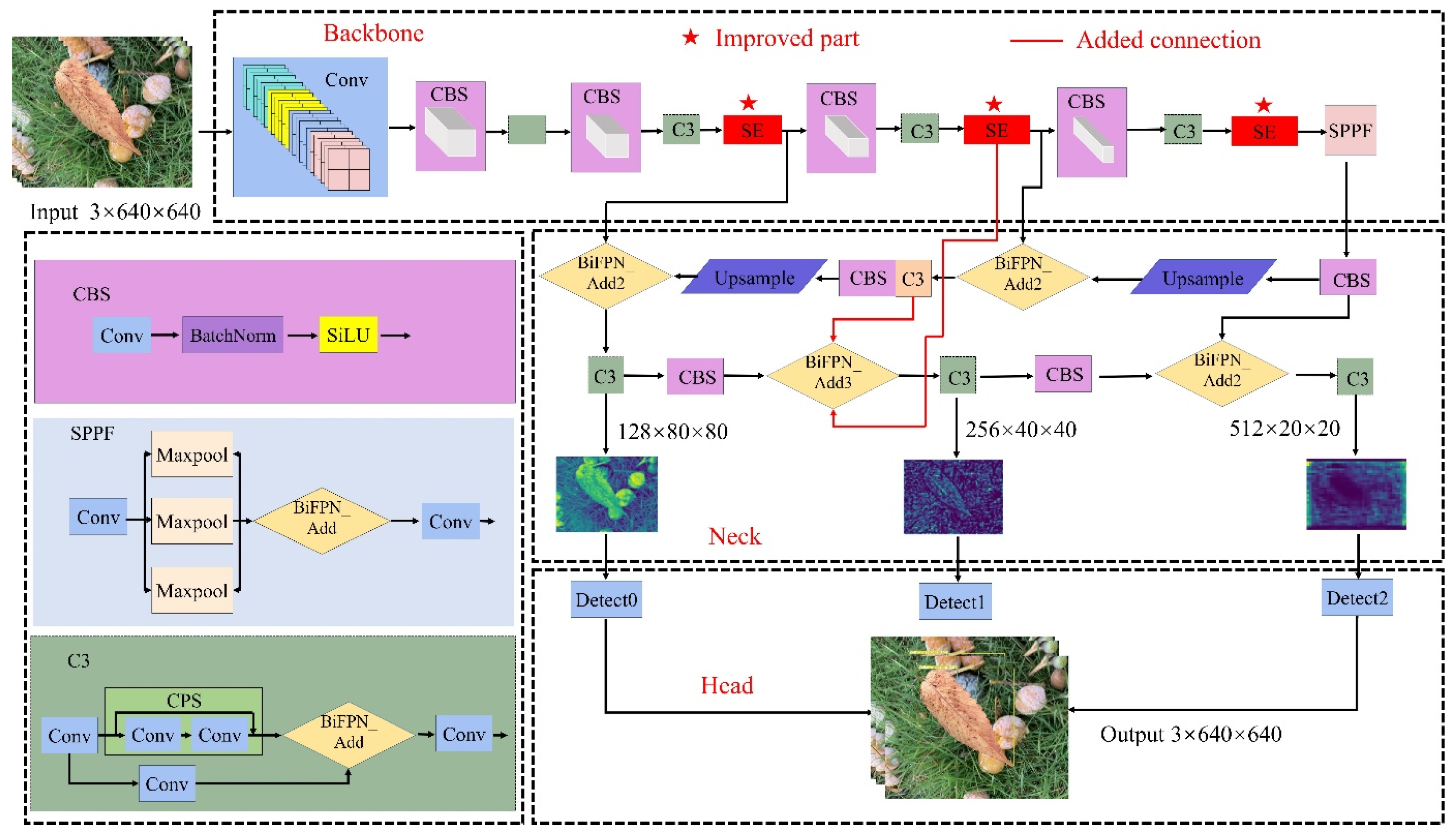
2.2. Model Architecture and Configuration

In the YOLO (You Only Look Once) series, YOLOv1 [16] lays the foundation for the entire series, and all other versions of YOLO improve on the first version. YOLOv1 innovatively uses a single-stage structure for the classification and object localization tasks, but it has a small receptive field and unspecific network losses. YOLOv2 [17] introduces batch normalization, which removes the fully connected layer and further improves the performance of the model. YOLOv3 [18] adds a detection box prediction function to YOLOv2 and uses Darknet-53 to extract features. Based on the above object detection architecture, YOLOv4 [19] optimizes algorithms of different degrees in data processing, backbone training, activation function, loss function, etc. YOLOv5 [20] makes some new improvements based on YOLOv4, and the speed and accuracy are greatly improved. YOLOv5 can be classified into YOLOv5n and YOLOv5s according to the depth and width of the model, as well as YOLOv5m, YOLOv5l, and YOLOv5x, totaling five network structures. The width of the model refers to the number of channels in each layer or feature extraction block of the network. Increasing the width means adding more channels to each layer, which can aid the network in capturing more information and features but also leads to increased computational load and model size. The depth of the model pertains to the number of layers in the network. Adding depth implies introducing more layers, aiding the model in learning more complex features and patterns. However, an overly deep network may encounter training difficulties, such as vanishing or exploding gradients. The structural parameters of the five YOLOv5 versions are shown in

Table 2. Network structures of the YOLOv5 series. The values for width and depth are scaling factors, representing the proportional scaling of the various YOLOv5 variants in width and depth relative to the baseline.

Model	Width	Depth	Params (M)	Size (MB)
YOLOv5n	0.25	0.33	1.90	3.90
YOLOv5s	0.50	0.33	56.80	14.10
YOLOv5m	0.75	0.67	64.10	40.80
YOLOv5l	1.00	1.00	67.30	89.40
YOLOv5x	1.25	1.33	68.90	167.00

. Among them, YOLOv5s offers better real-time detection and reduces training and deployment costs. Considering the trade-off between detection accuracy and detection speed, this study minimizes the degradation of detection speed while significantly improving detection accuracy. Therefore, this paper chooses to optimize and improve YOLOv5s.

In order to improve the detection performance for single leaves, this study proposes SinL-YOLOv5 based on YOLOv5s, and its network structure is shown in Figure 4.

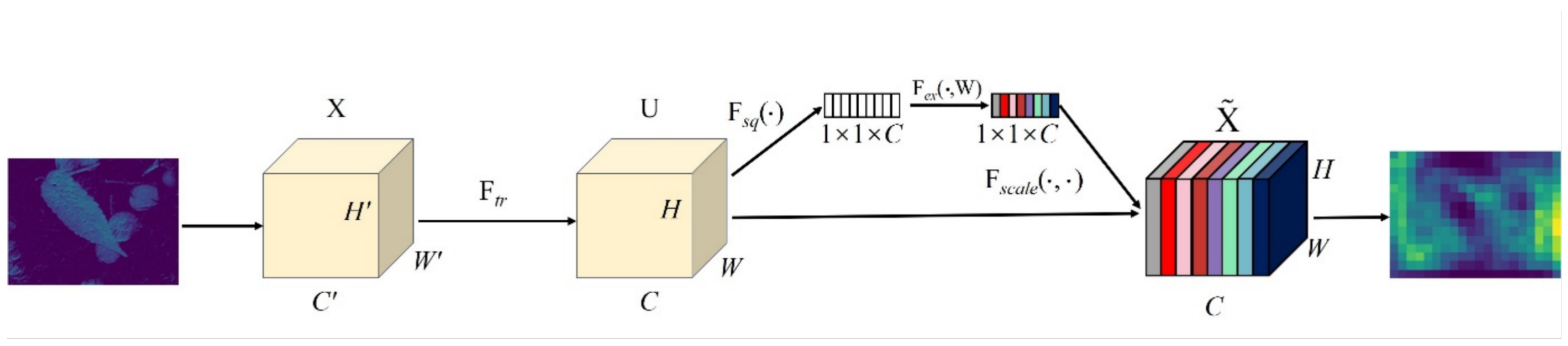
2.2.1. Backbone with SE Modules

In the traditional convolutional pooling process, each channel of the feature mapping is considered equally important. However, the importance of different channels differs. The channels enable the model to simultaneously extract features from the image at multiple angles and levels. Multiple convolutional kernels allow convolutional operations to be performed on different channels of the input image to extract different feature information. This feature information can be further combined, abstracted, and transformed in subsequent layers for more advanced image recognition and analysis tasks. The dimensions of the channel are closely related to the texture features learned by the model. Increasing the dimensions of the channel can improve the model’s ability to abstract and extract different features, but at the same time, it also increases the complexity of the model and the number of parameters. Therefore, it is crucial to choose the appropriate channel dimensions.

In order to address the problem of loss due to the varying importance of different channels in the feature mapping during the convolutional pooling process, this paper introduces the SE attention mechanism in SinL-YOLOv5. This mechanism aims to enhance the model’s ability to capture correlations between features and represent feature information more effectively. The SE module increases attention to channel dimensions, with key operations involving squeezing and excitation. In this way, the SE module focuses the neural network on some feature channels through automatic learning. The SE module can improve useful feature channels for the current task while suppressing those that are not useful for the current task. Therefore, SE can significantly improve model performance with only a slight increase in computational cost.

A schematic diagram of the SE module is shown in Figure 5. Before the feature map of the backbone network is input to the SE attention module, the importance of each channel in the feature map is the same. After the feature map is processed by SE, the importance of each feature channel is different. Different colors represent different weights, indicating that the neural network focuses more on channels with larger weights.

As shown in Figure 5, $F_{sq}$ is a squeezing operation on U, which is equivalent to a global average pooling operation performed on the vectors of each channel to obtain the global information corresponding to each channel. The formula is as follows:

$$Z_c=F_{sq}\left(u_c\right)=\frac{1}{H\times W}\sum _{i=1}^H\sum _{j=1}^W{u}_c(i,j)$$

(1)

where $Z_c$ is the output of the $F_{sq}$ operation, with the subscript c denoting the channel; $u_c$ denotes the c-th two-dimensional matrix in U; and ${\sum }_{i=1}^H{\sum }_{j=1}^W{u}_c(i,j)$ represents the summation over each pixel in the matrix $u_c$.

After the $F_{sq}$ operation is applied to all channels, the input of size $H\times W\times C$ is transformed into an output of size $1\times 1\times C$.

$F_{ex}$ is the incentive operation, which is equivalent to two fully connected operations, and it is formulated as follows:

$$S=F_{ex}(z,w)=\sigma \left({\omega }_2\sigma \left({\omega }_{1}z\right)\right)$$

(2)

where S is the output of the $F_{ex}$ operation; z is the $1\times 1\times C$ vector output from the $F_{sq}$ operation; $\omega$ is the weight matrix used to perform the excitation operation on z; and $\sigma$ is the activation function, which can be ReLU or Sigmoid.

The resulting S is subjected to the $F_{scale}$ operation, where the weights $s_c$ of each channel and the feature map $u_c$ are multiplied according to the channels to obtain the weighted $\tilde{X}$, which can be expressed as

$$\widetilde{X_c}=F_{sacle}(u_c,s_c)=s_c{u}_c$$

(3)

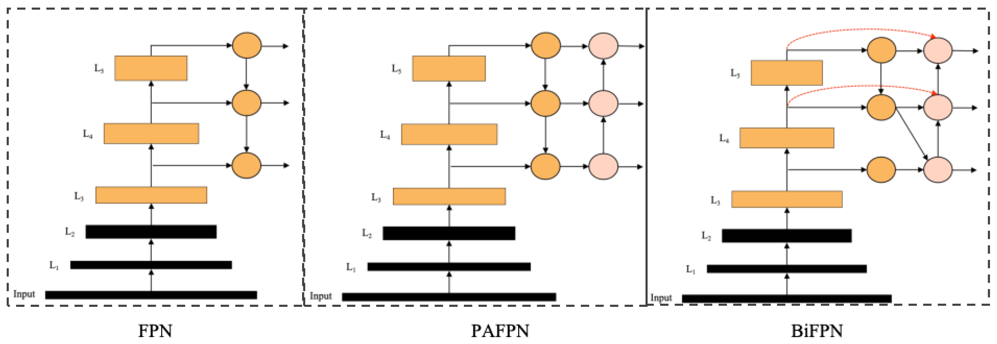
2.2.2. SE-BiFPN Architecture

In YOLO, feature maps are generated through a series of convolutional operations applied to the original image, and these feature maps can represent the characteristics of the original image at multiple scales. As the depth of the neural network increases, the backbone network outputs feature maps at different scales. Feature maps of different scales refer to the feature representations extracted by the neural network at various depth levels, each with different spatial resolutions. Shallow layers, such as $L_3$, output large-scale feature maps, which retain more spatial details of the original image, and lower-level features, such as edges and textures. Deeper layers, like $L_5$, output small-scale feature maps that represent more abstract and higher-level feature representations, such as the overall object. As the model deepens, these feature maps decrease in spatial dimensions but often have more channels, containing more complex and targeted feature information.

Larger feature maps tend to capture more global and abstract information, while smaller feature maps can provide finer details about local features. However, there is a potential for feature information to be lost during the transmission process in deeper layers of the network. Therefore, multi-scale feature fusion techniques, which integrate feature maps of different scales, have been developed. These techniques simultaneously learn and utilize both global and local information, making the model more powerful and flexible. Currently, common feature fusion architectures include the Bidirectional Feature Pyramid Network (BiFPN), the Panoptic Feature Pyramid Network (PAFPN), and the Feature Pyramid Network (FPN). These three feature fusion architectures are illustrated in Figure 6.

As shown in Figure 6, $L_5$ represents a deeper layer of the network, outputting smaller-sized feature maps, whereas $L_3$ is a shallower layer, outputting larger-sized feature maps. FPN adopts a top-down strategy to construct feature pyramids, successfully integrating deep and shallow features, as well as multi-scale information, but there are limitations in its unidirectional feature flow paths. PANet adds bottom-up loops on top of FPNs. PANet adds a bottom-up loop to the FPN to provide one more chance for feature fusion. BiFPN, on the other hand, improves the weighted path for bidirectional flow and optimizes the fusion process of multi-scale features, which is both efficient and fast.

This study aims to further improve the retention rate and accuracy of object features in detection and, therefore, proposes a new network architecture, SE-BiFPN. This architecture combines the advantages of the SE module and the BiFPN structure, takes full advantage of the SE’s channel attention mechanism to optimize the feature weights, and improves the utilization efficiency and accuracy of the feature information based on BiFPN, significantly improving object detection. The structure is shown in Figure 7. With SE-BiFPN, this study ensures the effectiveness and completeness of the network in extracting deep learning features, thereby achieving higher detection accuracy.

As shown in Figure 7, the SE layer in the backbone network is first utilized to adaptively capture feature maps at different scales. Next, lateral connectivity and downsampling operations are implemented to accomplish the first feature fusion. Then, the jump connectivity technique is used to combine the downsampling and upsampling processes of feature maps at the same scale for the second feature fusion. Finally, the resulting feature maps are obtained after these multi-scale fusions. Taking the fourth channel as an example, the feature maps processed through the SE module, along with intermediate feature mappings and final feature map outputs in the feature fusion process, are presented as follows:

$$L_4^{td}=Conv(\frac{a_1\times L_4^{SE}+a_2\times R(L_5^{SE})}{a_1+a_2+\gamma })$$

(4)

$$L_4^{out}=Conv(\frac{a_1^{\prime }\times L_4^{SE}+a_2^{\prime }\times L_4^{td}+a_3^{\prime }\times R(L_3^{out})}{a_1^{\prime }+a_2^{\prime }+a_3^{\prime }+\gamma })$$

(5)

where $L_i^{SE}$ represents the input features after being processed by the SE module at the i-th layer; $L_i^{td}$ is the intermediate feature of the i-th layer on the top-down path; $L_i^{out}$ is the output feature of the i-th layer on the bottom-up path; $Conv$ is the convolution operation of feature processing; R represents the upsampling or downsampling operation of resolution matching; a is a parameter we trained to distinguish the importance of different features in the process of feature fusion; and $\gamma$ is a preset smaller value to avoid numerical instability, which is usually set to 0.0001.

The BiFPN network enhances the capability to fuse shallow and deep feature information from images. The features extracted by the SinL-YOLOv5 backbone network are first processed through the SE module and then repeatedly fed into the BiFPN structure. This implementation facilitates bidirectional multi-scale feature fusion, improves the model’s ability to learn holistic features, and reduces the rate of misidentification.

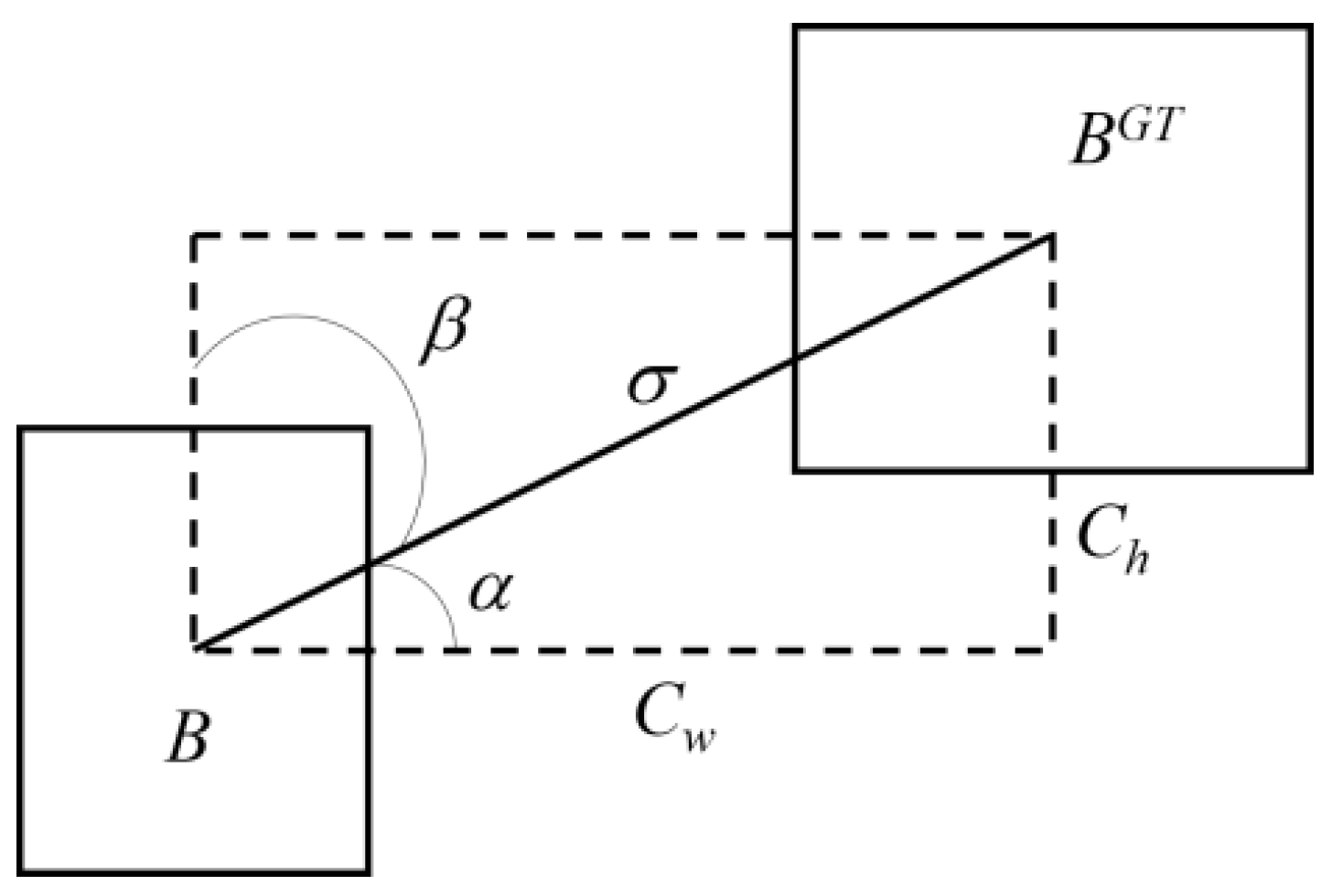
2.2.3. SIoU Loss Function

IoU is a standard metric used in object detection to assess the fit of predicted boxes to ground-truth boxes. However, it does not fully consider the differences in size, shape, and location between object boxes, which limits its accuracy. For this reason, improved methods such as GIoU [37], DIoU [38], and CIoU [39] have been proposed, which compensate for IoU’s shortcomings in terms of shape, position, and scale by adding compensating factors. GIoU considers the intersection ratio of the smallest outer rectangle, CIoU incorporates the distance and scale factors of the object boxes, and DIoU synthesizes the relative distances and aspect ratios between the object boxes. Despite the improvements of each of these methods, they still suffer from computational complexity or insufficient adaptability to objects of specific shapes. For more effective detection of a single leaf with large-scale variations, Zhora et al. [40] proposed the SIoU loss function. SIoU not only calculates the intersection and concatenation of boxes but also pays special attention to the scale variations between object boxes. This allows the model to be more robust with respect to multi-scale features of objects such as leaves, aiming to achieve more accurate and adaptable single-species leaf detection.

In the task of detecting key features of leaves, the model must be able to accurately recognize the specific morphology of a single leaf. Due to the diversity of leaves in their natural state, their shape, size, texture, and other features vary significantly, and adapting the model to these morphological variations is critical. The CIoU loss function used in the traditional YOLOv5s algorithm mainly focuses on the position and scale of the predicted box and the ground-truth box but does not fully consider the consistency of the morphology, which limits the recognition accuracy of the model to some extent. In contrast, the SIoU loss function introduces the consideration of morphological similarity between the predicted box and the ground-truth box, and by optimizing the shape-matching degree, it can further improve detection accuracy and the robustness of the model. During the iterative training process of neural networks, calculating the deviation of the predicted value from the ground-truth value generated in each iteration and correcting it is an important step to facilitate the progress of model optimization toward the ideal convergence state. Therefore, in order to accelerate convergence speed and improve the performance of the SinL-YOLOv5 model in the task of leaf detection, this study adopted the SIoU loss function instead of the original CIoU. This improvement not only significantly strengthens the model in terms of convergence but also results in excellent detection performance in recognizing various types of leaves.

The goal of SIoU is to predict the model on either the X or the Y axis, followed by approximation along the relevant axis. First, we try to minimize the angle. As shown in Figure 8, when $\alpha$ is $\frac{\pi }{2}$ or 0, the angle loss is 0. During the training process, if $\alpha \le \frac{\pi }{4}$, we minimize $\alpha$; otherwise, we minimize $\beta =\frac{\pi }{2}-\alpha$.

We also introduce the angular costing formula:

$$\Lambda =cos(2\times (arcsin(\frac{c_h}{\sigma })-\frac{\pi }{4}))$$

(6)

where $\sigma =\sqrt{{(b_{c_x}^{gt}-b_{c_x})}^2+{(b_{c_y}^{gt}-b_{c_y})}^2}$ and $c_h=max(b_{c_y}^{gt},b_{c_y})-min(b_{c_y}^{gt},b_{c_y})$. $\sigma$ is the distance between the center point of the ground-truth box and the predicted box, and $c_h$ is the height difference between the center point of the ground-truth box and the predicted box. $b_{c_x}^{gt}$ and $b_{c_y}^{gt}$ are the coordinates of the center of the ground-truth box. $b_{c_x}$ and $b_{c_y}$ are the coordinates of the center of the predicted box.

Angle costing was applied to distance costing by introducing angle costing into distance costing and redefining distance costing as follows:

$$\Delta =\sum _{t=x,y}{(1-e^{-\gamma \rho t})}^2=2-e^{-\gamma \rho x}-e^{-\gamma \rho y}$$

(7)

where $\rho ={(\frac{b_{c_x}^{gt}-b_{c_x}}{c_w})}^2$, ${\rho }_y=\frac{b_{c_y}^{gt}-b_{c_y}}{c_h}$, and $\gamma =2-\Lambda$. $c_w$ and $c_h$ are the width and height of the smallest outer rectangle of the ground-truth and predicted boxes.

The shape loss is defined as

$$\Omega =\sum _{t=w,h}{(1-e^{-w_t})}^{\theta }={(1-e^{-w_w})}^{\theta }+{(1-e^{-w_h})}^{\theta }$$

(8)

where $w_w=\frac{|w=w^{gt}|}{max(w,w^{gt})}$ and $w_h=\frac{|h=h^{gt}|}{max(h,h^{gt})}$. $(w,h)$ and $(w^{gt},h^{gt})$ are the width and height of the predicted and ground-truth boxes, and $\theta$ is the shape loss concern factor.

Finally, the SIoU loss function is defined as

$$Los{s}_{SIoU}=1-IoU+\frac{\Delta +\Omega }{2}$$

(9)

2.2.4. Experimental Environment

Our experiments were conducted on an experimental platform equipped with an Intel(R) Xeon(R) E5-4627 v4 CPU @ 2.60 GHz from Intel, Santa Clara, CA, USA, 64 GB of RAM, and an NVIDIA GeForce RTX 2080Ti 11G from NVIDIA, Santa Clara, CA, USA. The software environment was configured with CUDA11.7.0, Pytorch 2.0, and Python 3.10. Considering the performance of the hardware devices and the training effect, this paper adopted the batch training method to divide the training and validation processes into multiple batches. During the model’s training process, the size of the images was normalized to $640\times 640$ pixels as input to the network, and the learning rate was updated using the StepLR mechanism. The optimizer used was SGD Momentum. The values of Momentum and the other training parameters are detailed in

Table 3. Values of training parameters.

Project	Value
Momentum	0.95
Weight decay	0.0005
Batch size	16
Workers thread	12
Initial learning rate	0.01
Final learning rate	0.1
Epochs	300
Thresh	0.5
Image size	$640\times 640$ pixels

.

2.2.5. Accuracy Measurements

In order to objectively evaluate the model’s performance in detecting different leaves, this paper focuses on balancing the model’s performance in terms of two aspects: model performance and complexity. In the performance aspect, this paper uses the mean average precision ($mAP$), loss function value (loss), precision (P), and recall (R) to evaluate the performance of the evaluation model. The loss function value curve is used to reflect the change in the loss function value during model training. It can intuitively reflect the difference between the predicted value and the ground-truth value of the model during the training process, such that the smaller the difference, the higher the prediction accuracy of the model and the better the performance of the model. P is a measure of the proportion of positive samples correctly predicted by the model to all positive samples, such that the higher the precision rate, the higher the number of positive samples correctly predicted by the model and the better the performance of the model. R refers to the proportion of positive samples correctly predicted by the model to all positive samples that are actually positive, such that the higher the recall rate, the more real objects the model can detect and the better the performance of the model. The $mAP$ is an important index for evaluating the detection effect of the object detection model, such that the higher the value, the higher the average detection accuracy of the model and the better the performance of the model. The $mAP$ is calculated as the average of the $AP$ across all classes. Here, the $AP$ represents the precision–recall curve’s area under each class. The formulas are as follows:

$$P=\frac{TP}{TP+FP}$$

(10)

$$P=\frac{TP}{TP+FN}$$

(11)

$$AP={\int }_0^{1}P\left(R\right)dR$$

(12)

$$mAP=\frac{{\sum }_{n=1}^{N}AP\left(n\right)}{N}$$

(13)

where $TP$ represents true positives, the number of correct positive predictions made by the model; $FP$ represents false positives, the number of incorrect positive predictions made by the model; and $FN$ represents false negatives, the number of positive instances that were not correctly predicted by the model.

In terms of model complexity, three main metrics are considered: the number of parameters, the number of floating points of operations (FLOPs), and the model size [41]. FLOP denotes the speed of floating-point operations, which is calculated by counting the total number of floating-point operations in the model, and it can be used to measure the complexity of the model. Parameters represent the computational memory resources consumed by the model. The formulas are as follows:

$$Parameters=r\times f^2\times g+g$$

(14)

$$FLOPs=2\times H\times W\times C_{out}\times (C_{in}\times K^2+1)$$

(15)

where r is the input size, f is the convolutional kernel size, g is the output size, $H\times W$ is the output feature map size, $C_{in}$ is the input channel, K is the kernel size, and $C_{out}$ is the output channel.

3. Results and Discussion

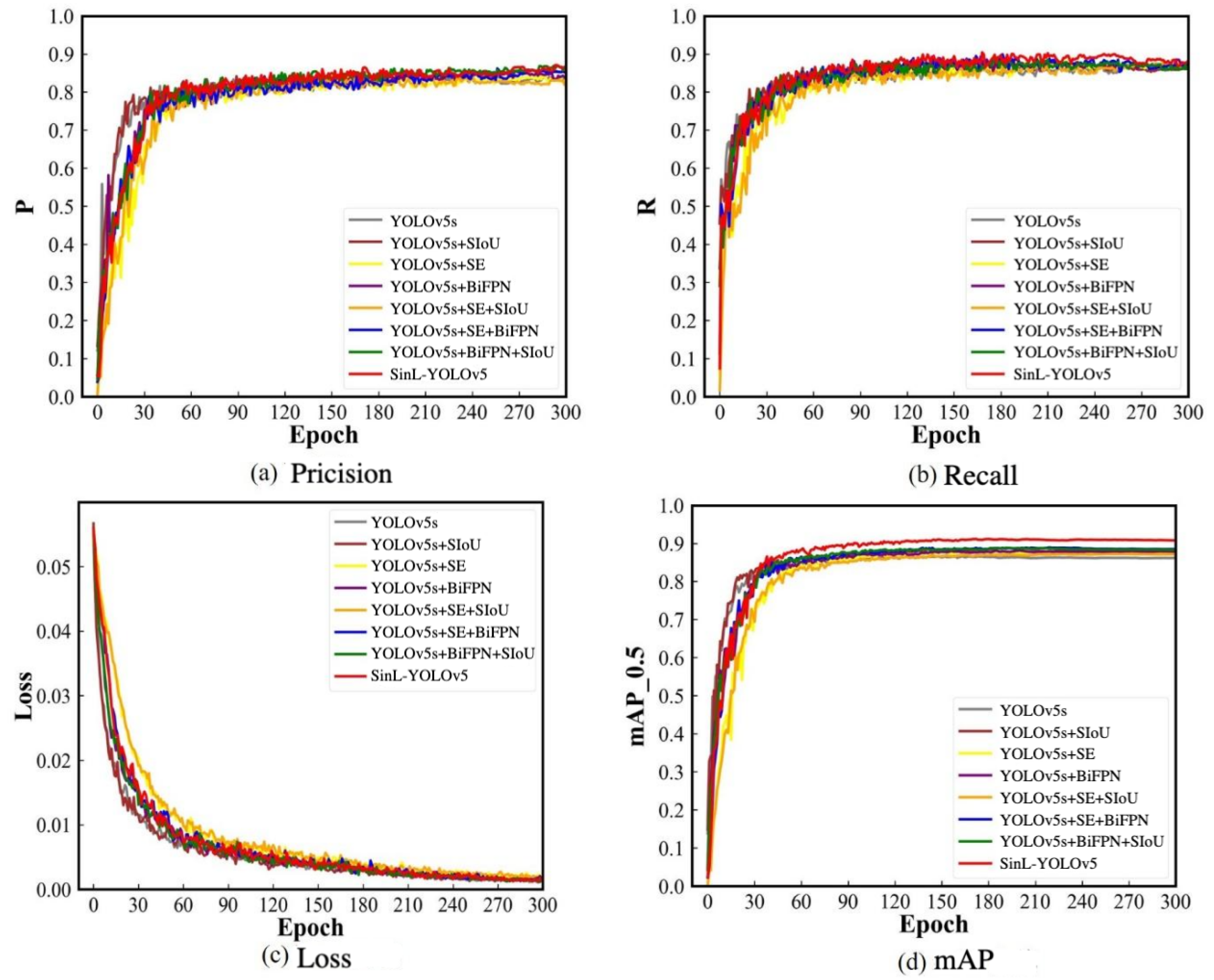
3.1. Model Performance and Ablation Experiment

To validate the effectiveness of the different modules, this study conducted a series of ablation tests for a total of eight different models. The results of the ablation tests are shown in

Table 4. Ablation experiment.

Model	FLOPs (G)	Params (M)	[email protected] (%)	[email protected]:0.95 (%)	Size (MB)
YOLOv5s	15.80	7.03	86.10	74.30	14.40
YOLOv5s + SIoU	15.80	7.03	87.70	75.90	14.40
YOLOv5s + SE	16.90	7.88	87.60	73.70	14.40
YOLOv5s + BiFPN	16.40	7.18	87.90	74.70	14.70
YOLOv5s + SE + SIoU	16.90	7.88	87.10	73.00	16.10
YOLOv5s + SE + BiFPN	16.90	7.70	88.50	74.60	15.70
YOLOv5s + SIoU + BiFPN	16.40	7.18	88.40	75.20	14.70
SinL-YOLOv5	16.90	7.70	90.80	76.90	15.70

.

As shown in Table 4, the embedded modules had a positive impact on the mAP values in our study. The attention mechanism of the SE module selectively focused on informative features, increasing the model’s [email protected] by 1.5%. The architecture combining SE with BiFPN enhanced the model’s feature fusion capabilities, raising the [email protected] by 2.4%. The SIoU learned more effective leaf edge positioning and sizing, improving the [email protected] by 1.6%. Table 4 also demonstrates that combining all three modules yielded higher detection and recognition accuracy compared to integrating just one or two modules. The number of parameters and the computational complexity of SinL-YOLOv5 increased slightly compared to YOLOv5s, but the [email protected] and the [email protected]:0.95 reached 90.80% and 76.90%, an improvement of 4.6% and 2.6%, respectively. In terms of model complexity, the parameters, FLOPs, and model size of the improved model increased by 6.50%, 8.70%, and 8.2%, respectively, over the original YOLOv5s network. Although the introduction of more parameters and computations can impact the computational efficiency of the model, these adjustments resulted in significant performance improvements, especially in terms of the robustness of the model’s detection performance. In addition, the robustness of the model is directly related to its reliability in real-world applications, so this performance enhancement means that the improved model can achieve accurate detection in more diverse environments and conditions. At the same time, although the complexity increased, this trade-off in complexity is justified as it supports the enhancement of the model’s generalization ability and accuracy.

The precision, recall, loss, and mAP curves for the eight models are shown in Figure 9.

In Figure 9a,b, it can be seen that the improved SinL-YOLOv5 significantly outperformed the standard YOLOv5s model in terms of precision and recall.

In Figure 9c, the continuous iteration of the model illustrates the change in the loss function, which can be intuitively observed to see whether the model steadily converged toward optimization as the iterations progressed. The loss curve of SinL-YOLOv5 decreased and tended to be steady as the iterations progressed, and the loss value reached a steady state at about 270 iterations, signifying that the model basically reached convergence. Compared with YOLOv5s, SinL-YOLOv5 demonstrated a faster convergence speed. The mAP value is an important indicator of the effectiveness of the object detection model, and an increase in the mAP value implies that the model’s average detection accuracy has been enhanced, resulting in improved performance. As shown in Figure 9d, the [email protected] value of SinL-YOLOv5 was close to 90%, and after approximately 180 iterations, the value increased to a peak of 90.8%. Compared with YOLOv5s, SinL-YOLOv5 improved the [email protected] value by nearly 4.7 percentage points, significantly enhancing detection accuracy. The experimental results show that SinL-YOLOv5 is capable of accurately recognizing various types of leaf objects.

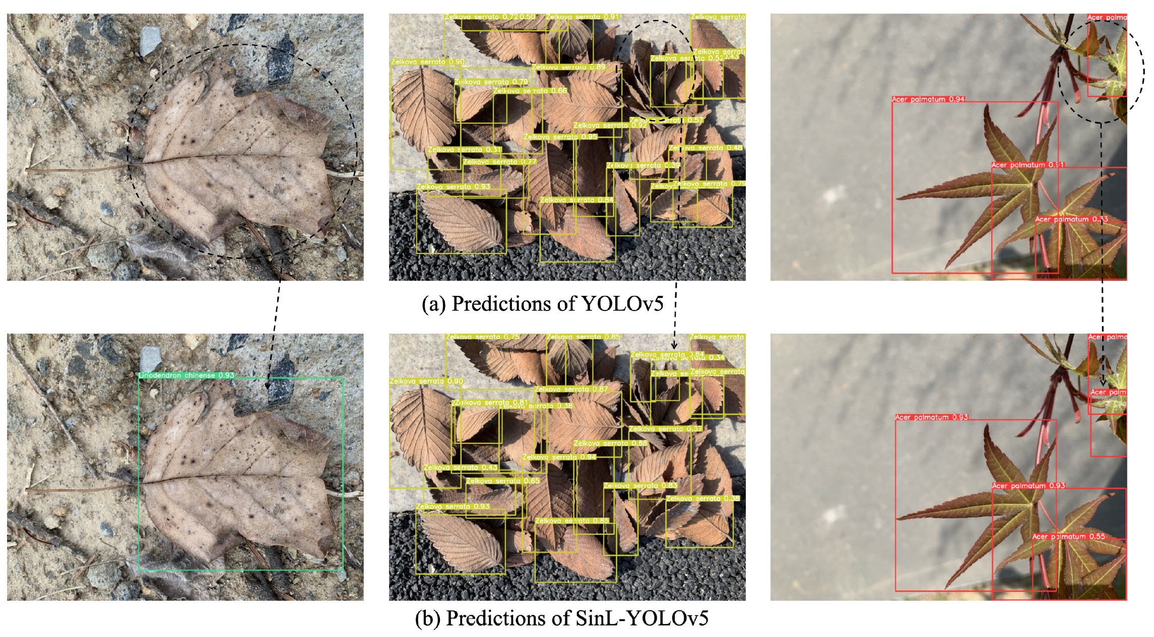
3.2. Comparative Experiment

In this paper, six mainstream models were selected for comparison to verify the effectiveness of the proposed model. The model was compared with the classical SSD, YOLOv3, YOLOv4, EfficientDet [42], Faster R-CNN, and YOLOv5s models using the above experimental environment and parameter settings. The results are shown in

Table 5. Comparative experiment.

Model	P (%)	R (%)	[email protected] (%)	[email protected]:0.95 (%)	FPS	Size (MB)
SSD	66.13	65.72	65.88	54.10	74	91.60
YOLOv3	66.82	67.06	67.51	60.60	55	236.00
YOLOv4	80.77	65.16	71.52	63.70	43	244.00
EfficientDet	86.30	69.64	77.65	57.00	36	15.00
Faster R-CNN	84.85	80.48	84.59	71.10	10	108.00
YOLOv5s	83.60	86.30	86.10	74.30	62	14.40
SinL-YOLOv5	86.50	87.50	90.80	76.90	82	15.70

.

The data in Table 5 clearly demonstrate the significant advantages of SinL-YOLOv5 over the other six models in terms of accuracy. Specifically, SinL-YOLOv5 achieved high levels of accuracy, recall, [email protected], and [email protected]:0.95 evaluation criteria. Although the number of parameters and computations of SinL-YOLOv5 increased slightly from the pre-improvement period to the post-improvement period, the performance of the model improved. Compared to YOLOv5s, the precision, recall, [email protected], and [email protected]:0.95 of SinL-YOLOv5 improved by 2.9%, 1.2%, 4.7%, and 2.6%, respectively. This performance improvement is especially significant for the real-time accurate identification of single-species leaves. In this application scenario, SinL-YOLOv5 demonstrated exceptional detection speed, capable of processing 82 frames per second, which is higher than the rates achieved by the six classic models compared. Additionally, our model maintained a relatively small size, fully meeting the dual requirements of processing speed and recognition accuracy in complex environments.

In order to realize leaf detection in complex environments, this paper selected images with different backgrounds, such as varying lighting, partial occlusions, and the presence of different objects, to verify the robustness of the model before and after improvement, as shown in Figure 10.

During actual prediction, the complexity of the background among the leaves, partial occlusions, and the presence of small object areas in the images resulted in some information loss, which posed challenges to accurately identifying key information about the leaves. As seen in Figure 10a, YOLOv5s lacked the capability to differentiate between various leaves, leading to false positives and missed detections. Due to factors such as the similarity between the leaves and the background, overlapping leaves, and significant size variations among leaves, YOLOv5s exhibited inferior overall feature extraction capabilities. Based on this, our study added an SE module to the YOLOv5s model to enhance its ability to capture diverse local information. We introduced SIoU to integrate directional information between ground-truth boxes and predicted boxes, effectively improving the learning of leaf edge positioning and sizing. Moreover, we merged the backbone of YOLOv5s with the proposed SE-BiFPN structure. This integration not only reduced feature information loss in tasks with similar backgrounds and small object detection but also enhanced object detection accuracy, compensating for the deficiencies of the YOLOv5s algorithm. The detection results are shown in Figure 10b.

4. Conclusions

In this study, we selected leaves from eight commonly seen landscape trees in Chinese cities, which are similar in shape and texture, as samples. The collected leaf images were screened and optimized to obtain a dataset suitable for urban real-world scenarios, featuring single species of trees against complex backgrounds. To more accurately learn the key and positional features of tree leaves in complex environments, this paper proposed a leaf key information detection model, SinL-YOLOv5, based on YOLOv5.

This model addresses the issue of feature map loss across different channels during the convolutional pooling process due to varying importance levels by integrating the SE module into the backbone network, which enhances the expression of key features such as leaf contours and textures. To combat the problem of feature loss, we proposed an improved feature fusion structure that strengthens the transfer of feature information between deep and shallow layers, enabling the model to better learn the connections between leaf shape textures and semantic information at different scales, thereby increasing the accuracy of object recognition. Additionally, we introduced a boundary box loss function based on angular cost (SIoU), which integrates directional information between ground-truth boxes and predicted boxes, more effectively learning the positioning and shape of leaf edges, thus enhancing the precision of leaf position detection.

Experimental results demonstrate that compared to YOLOv5s, the [email protected] value of SinL-YOLOv5 increased to 90.8%, an improvement of nearly 4.7 percentage points, significantly enhancing detection and recognition accuracy. Additionally, when compared with six other mainstream models, the SinL-YOLOv5 model achieved high levels of accuracy, recall, [email protected], and [email protected]:0.95 metrics. On the other hand, the size of the SinL-YOLOv5 model is only 15.70 MB. In the current landscape, where the cost of computational resources and storage space is increasingly expensive, this characteristic is particularly valuable. The smaller model size reduces the demand for storage and lowers the consumption of computational resources, making SinL-YOLOv5 an ideal choice for devices with limited resources. The SinL-YOLOv5 algorithm proposed in this paper balances performance and efficiency, providing a practical and efficient solution for fields such as intelligent forestry management and automated plant detection.

This study primarily focuses on the localization and recognition of tree leaves against complex urban backgrounds. Although the validation results for the eight types of tree leaves demonstrate the effectiveness of our developed model, there is still room for improvement in terms of sample diversity and leaf detection and recognition strategies. Therefore, we plan to further expand the size and diversity of the dataset by collecting leaves from more tree species, including extending the dataset of single-species leaves per image and creating a dataset with multiple species per image to enhance data diversity and coverage. This will not only improve the generalization of the model but also enhance its ability to handle tasks in complex and variable environments. Additionally, we will introduce a variety of data augmentation techniques to further improve the model’s adaptability to different environments, thereby enhancing its robustness. Furthermore, we will continue to improve the network structure of the existing model or newer models (such as Transformers), or reduce error loss from an algorithmic perspective to enhance the network’s representational capacity. This will further improve the model’s accuracy in detecting and recognizing leaves with similar backgrounds, overlapping leaves, and small object leaves.

All great scientific achievements begin with small, preliminary studies. While our current research has limitations, it is these small beginnings that pave the way to in-depth research and practical applications. By gradually expanding and deepening our research, we expect to provide innovative and practical solutions for the study and management of urban ecosystems.

References

1. Jianhui, D.; Jiajian, C.; Shengfa, L. Factors affecting thedisturbance: A review damage and recovery of coastal forest after typhoon. Acta Ecol. Sin. 2024, 44, 1–17. [Google Scholar] [CrossRef]
2. McPherson, E.G.; Van Doorn, N.; De Goede, J. Structure, function and value of street trees in California, USA. Urban For. Urban Green. 2016, 17, 104–115. [Google Scholar] [CrossRef]
3. Raj, J.N.; Rajeev, J.; Raj, M.J. Contribution of Urban Trees to Offset Carbon Dioxide Emissions from the Transportation Sector in the Ring Road Area of Kathmandu Valley, Central Himalaya. J. Resour. Ecol. 2023, 14, 1272. [Google Scholar] [CrossRef]
4. Yanzi, M.; Zongwei, Z.; Hesheng, W.; Wei, D.; Zhongxiang, Z.; Xiaolin, W.; Chunyu, Y.; Yannuo, S. Detection method of fallen leaves on road based on AC-YOLO. Control Decis. 2023, 38, 1878–1886. [Google Scholar] [CrossRef]
5. Sachar, S.; Kumar, A. Survey of feature extraction and classification techniques to identify plant through leaves. Expert Syst. Appl. 2021, 167, 114181. [Google Scholar] [CrossRef]
6. Xiaolong, Z. Study of Tree Leaf Recognition in Habitat Based on Deep Convolutional Neural Networks. Ph.D. Thesis, Northeast Forestry University, Harbin, China, 2020. [Google Scholar]
7. Yonekawa, S.; Sakai, N.; Kitani, O. Identification of idealized leaf types using simple dimensionless shape factors by image analysis. Trans. ASAE 1996, 39, 1525–1533. [Google Scholar] [CrossRef]
8. Wang, X.F.; Huang, D.S.; Du, J.X.; Xu, H.; Heutte, L. Classification of plant leaf images with complicated background. Appl. Math. Comput. 2008, 205, 916–926. [Google Scholar] [CrossRef]
9. Lei, W.; Dongjian, H.; Yongliang, Q. Plant Leaves Classification Based on Image Processing and SVM. J. Agric. Mech. Res. 2013, 35, 12–15. [Google Scholar]
10. Munisami, T.; Ramsurn, M.; Kishnah, S.; Pudaruth, S. Plant leaf recognition using shape features and colour histogram with K-nearest neighbour classifiers. Procedia Comput. Sci. 2015, 58, 740–747. [Google Scholar] [CrossRef]
11. Nian, L.; Jiangming, G. Plant leaf identifcation based on the multi-feature fusion and deep belief networks method. J. Beijing For. Univ. 2016, 38, 110–119. [Google Scholar] [CrossRef]
12. Longlong, L. Semi-Supervised Clustering and Its Application on Plant Leaf Image Recognition. Ph.D. Thesis, Northwest A&F University, Yangling, China, 2017. [Google Scholar]
13. Shanwen, Z.; Yu, S.; Ping, L. A plant recognition method based on global-local feature fusion by canonical correlation analysis. Jiangsu Agric. Sci. 2019, 47, 255–258. [Google Scholar] [CrossRef]
14. Leihong, W.; Yongsheng, C.; Yuhong, Z. Automatic ldentification of Elaeagnus L. Based on Leaf Digital Texture Feature. Chin. Agric. Sci. Bull. 2020, 36, 20–25. [Google Scholar]
15. Liu, W.; Anguelov, D.; Erhan, D.; Szegedy, C.; Reed, S.; Fu, C.Y.; Berg, A.C. Ssd: Single shot multibox detector. In Proceedings of the Computer Vision–ECCV 2016: 14th European Conference, Amsterdam, The Netherlands, 11–14 October 2016; pp. 21–37. [Google Scholar]
16. Redmon, J.; Divvala, S.; Girshick, R.; Farhadi, A. You only look once: Unified, real-time object detection. In Proceedings of the IEEE Conference on Computer Vision and Pattern Recognition, Las Vegas, NV, USA, 26 June–1 July 2016; pp. 779–788. [Google Scholar]
17. Redmon, J.; Farhadi, A. YOLO9000: Better, faster, stronger. In Proceedings of the IEEE Conference on Computer Vision and Pattern Recognition, Honolulu, HI, USA, 21–26 July 2017; pp. 7263–7271. [Google Scholar]
18. Redmon, J.; Farhadi, A. Yolov3: An incremental improvement. arXiv 2018, arXiv:1804.02767. [Google Scholar]
19. Bochkovskiy, A.; Wang, C.Y.; Liao, H.Y.M. Yolov4: Optimal speed and accuracy of object detection. arXiv 2020, arXiv:2004.10934. [Google Scholar]
20. Jocher, G.; Chaurasia, A.; Stoken, A.; Borovec, J.; NanoCode012; Kwon, Y.; Michael, K.; TaoXie; Fang, J.; imyhxy; et al. Ultralytics/yolov5: V7.0—YOLOv5 SOTA Realtime Instance Segmentation; Zenedo: Geneva, Switzerland, 2022. [Google Scholar] [CrossRef]
21. Girshick, R.; Donahue, J.; Darrell, T.; Malik, J. Rich feature hierarchies for accurate object detection and semantic segmentation. In Proceedings of the IEEE Conference on Computer Vision and Pattern Recognition, Columbus, OH, USA, 23–28 June 2014; pp. 580–587. [Google Scholar]
22. Girshick, R. Fast r-cnn. In Proceedings of the IEEE International Conference on Computer Vision, Santiago, Chile, 7–13 December 2015; pp. 1440–1448. [Google Scholar]
23. Ren, S.; He, K.; Girshick, R.; Sun, J. Faster R-CNN: Towards real-time object detection with region proposal networks. IEEE Trans. Pattern Anal. Mach. Intell. 2016, 39, 1137–1149. [Google Scholar] [CrossRef] [PubMed]
24. LeCun, Y.; Boser, B.; Denker, J.S.; Henderson, D.; Howard, R.E.; Hubbard, W.; Jackel, L.D. Backpropagation applied to handwritten zip code recognition. Neural Comput. 1989, 1, 541–551. [Google Scholar] [CrossRef]
25. LeCun, Y.; Bottou, L.; Bengio, Y.; Haffner, P. Gradient-based learning applied to document recognition. Proc. IEEE 1998, 86, 2278–2324. [Google Scholar] [CrossRef]
26. Shuai, Z.; Yongjian, H. Leaf image recognition based on layered convolutions neural network deep learning. J. Beijing For. Univ. 2016, 38, 108–115. [Google Scholar] [CrossRef]
27. Iwata, K. Extending the peak bandwidth of parameters for softmax selection in reinforcement learning. IEEE Trans. Neural Netw. Learn. Syst. 2016, 28, 1865–1877. [Google Scholar] [CrossRef]
28. He, K.; Zhang, X.; Ren, S.; Sun, J. Deep residual learning for image recognition. In Proceedings of the IEEE Conference on Computer Vision and Pattern Recognition, Las Vegas, NV, USA, 26 June–1 July 2016; pp. 770–778. [Google Scholar]
29. Jicheng, L.; Xiaobin, Y.; Daoxing, L.; Yixiang, S.; Senlin, Z. High similarity blade image recognition method based on HOG-CNN. Comput. Era 2019, 53–56. [Google Scholar] [CrossRef]
30. Zhe, X. Design and Analysis of Crop Leaf Recognition System Based on Deep Learning. Master’s Thesis, Jilin University, Changchun, China, 2019. [Google Scholar]
31. Szegedy, C.; Vanhoucke, V.; Ioffe, S.; Shlens, J.; Wojna, Z. Rethinking the inception architecture for computer vision. In Proceedings of the IEEE Conference on Computer Vision and Pattern Recognition, Las Vegas, NV, USA, 26 June–1 July 2016; pp. 2818–2826. [Google Scholar]
32. Liu, S.; Deng, W. Very deep convolutional neural network based image classification using small training sample size. In Proceedings of the 3rd IAPR Asian Conference on Pattern Recognition (ACPR), Kuala Lumpur, Malaysia, 3–6 November 2015; pp. 730–734. [Google Scholar]
33. Wu, S.G.; Bao, F.S.; Xu, E.Y.; Wang, Y.X.; Chang, Y.F.; Xiang, Q.L. A leaf recognition algorithm for plant classification using probabilistic neural network. In Proceedings of the IEEE International Symposium on Signal Processing and Information Technology, Giza, Egypt, 15–18 December 2007; pp. 11–16. [Google Scholar]
34. Kumar, N.; Belhumeur, P.N.; Biswas, A.; Jacobs, D.W.; Kress, W.J.; Lopez, I.C.; Soares, J.V. Leafsnap: A computer vision system for automatic plant species identification. In Proceedings of the Computer Vision—ECCV 2012: 12th European Conference on Computer Vision, Florence, Italy, 7–13 October 2012; pp. 502–516. [Google Scholar]
35. Söderkvist, O. Computer Vision Classification of Leaves from Swedish Trees. Professional Degree, Linköping University, Linköping, Sweden, 2001. [Google Scholar]
36. Shorten, C.; Khoshgoftaar, T.M. A survey on image data augmentation for deep learning. J. Big Data 2019, 6, 1–48. [Google Scholar] [CrossRef]
37. Rezatofighi, H.; Tsoi, N.; Gwak, J.; Sadeghian, A.; Reid, I.; Savarese, S. Generalized intersection over union: A metric and a loss for bounding box regression. In Proceedings of the IEEE/CVF Conference on Computer Vision and Pattern Recognition, Long Beach, CA, USA, 15–20 June 2019; pp. 658–666. [Google Scholar]
38. Zheng, Z.; Wang, P.; Liu, W.; Li, J.; Ye, R.; Ren, D. Distance-IoU loss: Faster and better learning for bounding box regression. In Proceedings of the AAAI Conference on Artificial Intelligence, New York, NY, USA, 7–12 February 2020; Volume 34, pp. 12993–13000. [Google Scholar]
39. Zheng, Z.; Wang, P.; Ren, D.; Liu, W.; Ye, R.; Hu, Q.; Zuo, W. Enhancing geometric factors in model learning and inference for object detection and instance segmentation. IEEE Trans. Cybern. 2021, 52, 8574–8586. [Google Scholar] [CrossRef] [PubMed]
40. Gevorgyan, Z. SIoU loss: More powerful learning for bounding box regression. arXiv 2022, arXiv:2205.12740. [Google Scholar]
41. Li, S.; Zhang, S.; Xue, J.; Sun, H. Lightweight target detection for the field flat jujube based on improved YOLOv5. Comput. Electron. Agric. 2022, 202, 107391. [Google Scholar] [CrossRef]
42. Tan, M.; Pang, R.; Le, Q.V. Efficientdet: Scalable and efficient object detection. In Proceedings of the IEEE/CVF Conference on Computer Vision and Pattern Recognition, Seattle, WA, USA, 14–19 June 2020; pp. 10781–10790. [Google Scholar]
Figure 1. The tree species in the dataset.
Forests 15 00894 g001
Figure 2. Examples of conditions for Liriodendron chinense.
Forests 15 00894 g002
Figure 3. Data enhancement results.
Forests 15 00894 g003
Figure 4. Network structure diagram of SinL-YOLOv5. The sections with asterisks are the improved sections, and the sections with solid red lines are the added links.
Forests 15 00894 g004
Figure 5. Structure of the SE module. X is the input feature map, F is the operation of the feature map, U is the feature map in the transformation whose size is H × W × C , and X ˜ is the feature map after scaling by the activation function.
Forests 15 00894 g005
Figure 6. Structures of FPN, PAFPN, and BiFPN.
Forests 15 00894 g006
Figure 7. Structure of SE-BiFPN module.
Forests 15 00894 g007
Figure 8. Schematic of SIoU angle.
Forests 15 00894 g008
Figure 9. Comparison of training results for different models.
Forests 15 00894 g009
Figure 10. Comparison of leaf detection results between YOLOv5s and SinL-YOLOv5.
Forests 15 00894 g010