
Estimation of Forest Canopy Fuel Moisture Content in Dali Prefecture by Combining Vegetation Indices and Canopy Radiative Transfer Models from MODIS Data


Abstract
1. Introduction
2. Materials and Methods
2.1. Materials
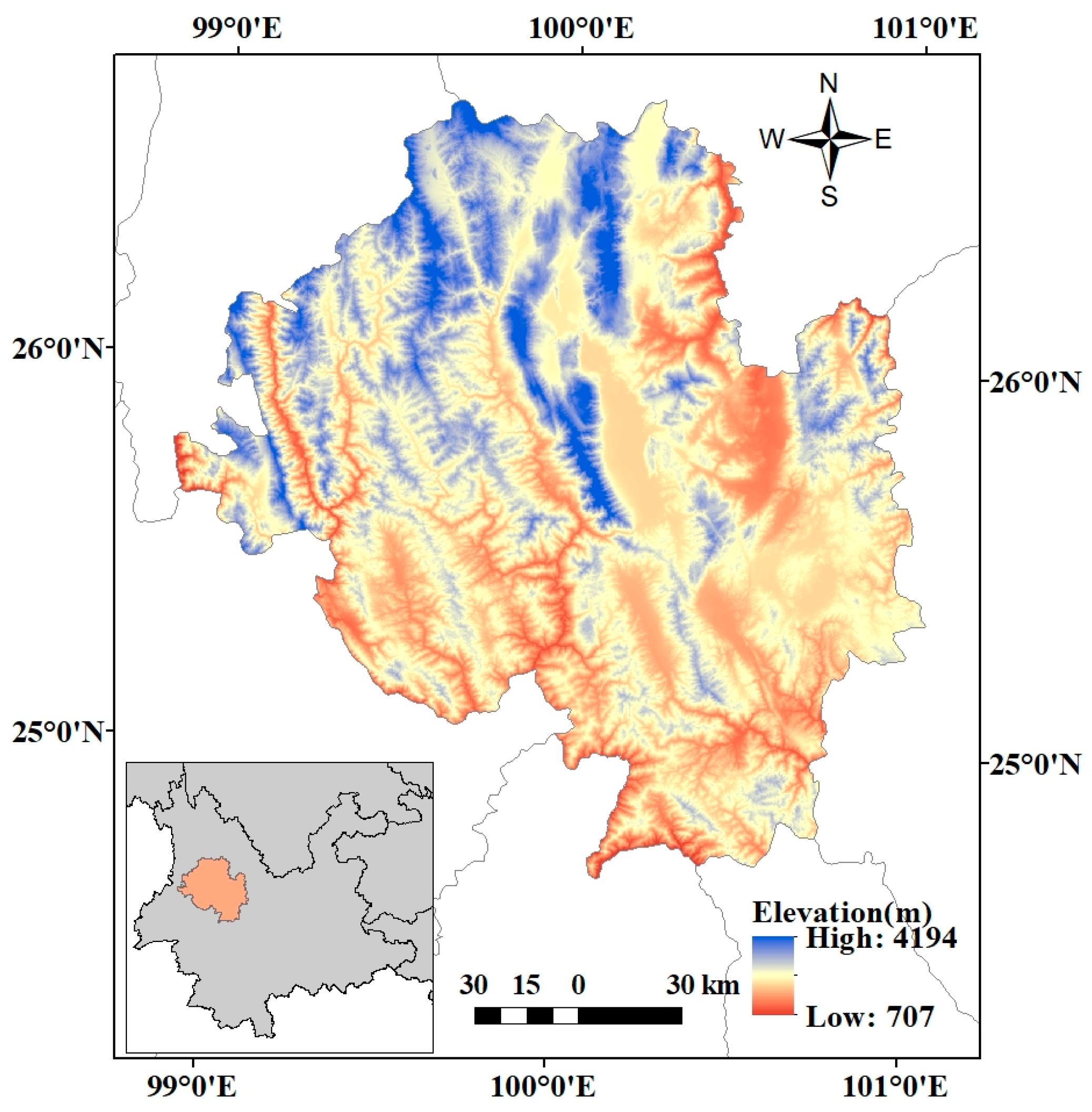
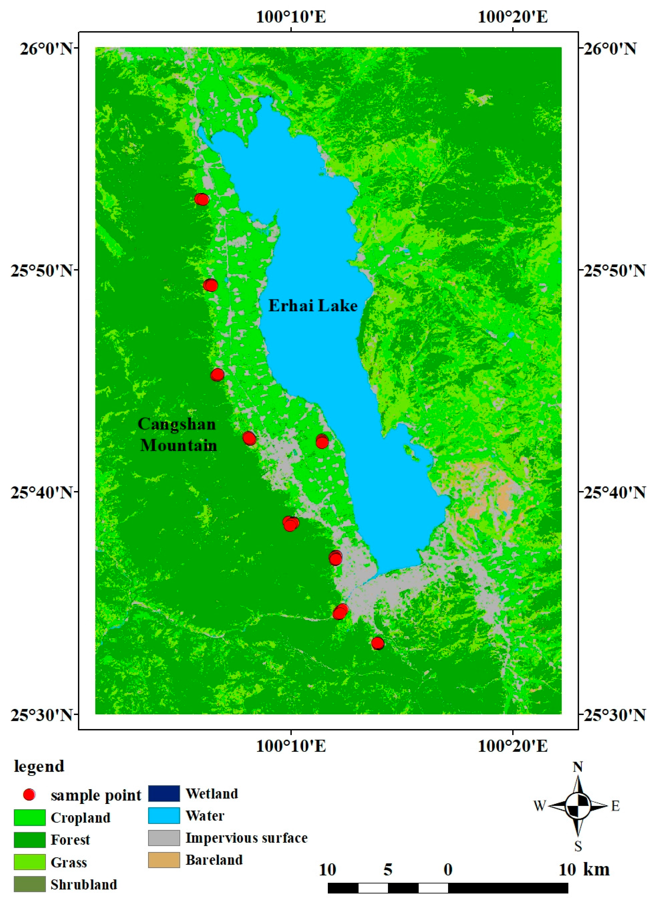
2.1.1. Study Area
2.1.2. MODIS Satellite Data
2.1.3. Field Data
2.2. Methods
2.2.1. Radiative Transfer Model
2.2.2. Sensitivity Analysis
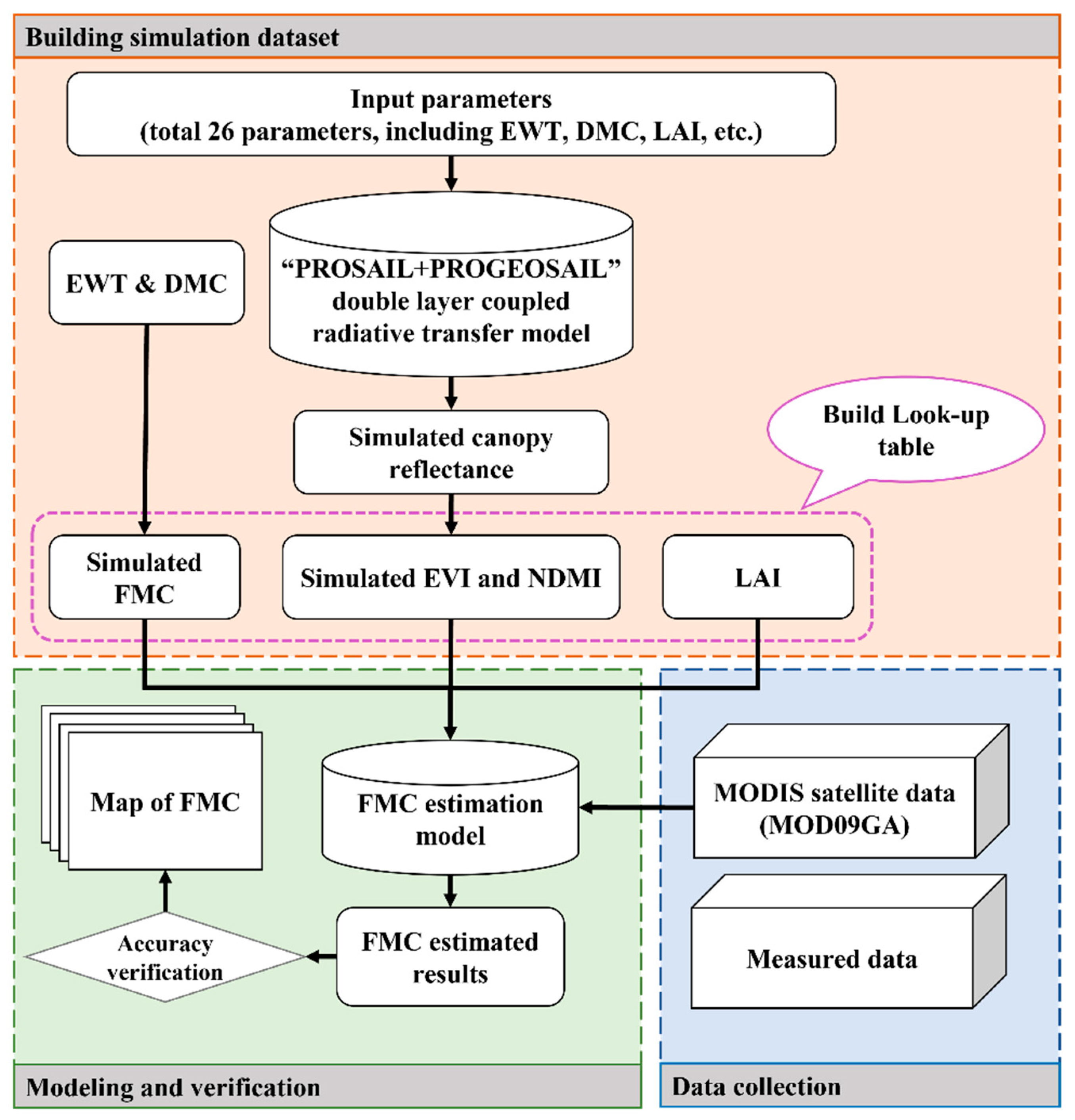
2.2.3. Construction of Total Look-Up Table
2.2.4. Correlation Analysis
2.2.5. Estimation of FMC
3. Results
3.1. Results of Sensitivity Analysis
3.2. Model Coefficient Matrix
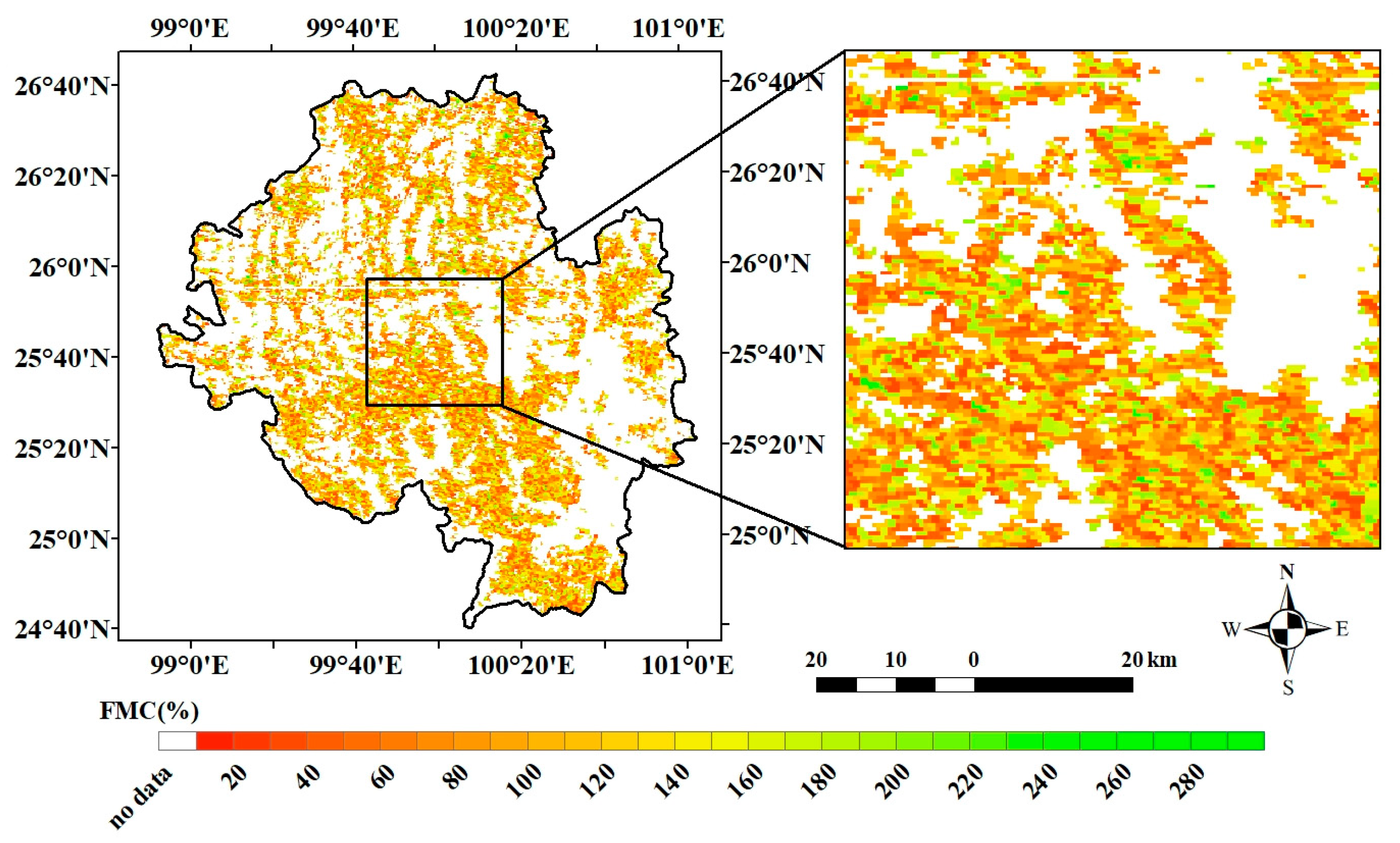
3.3. Mapping of FMC
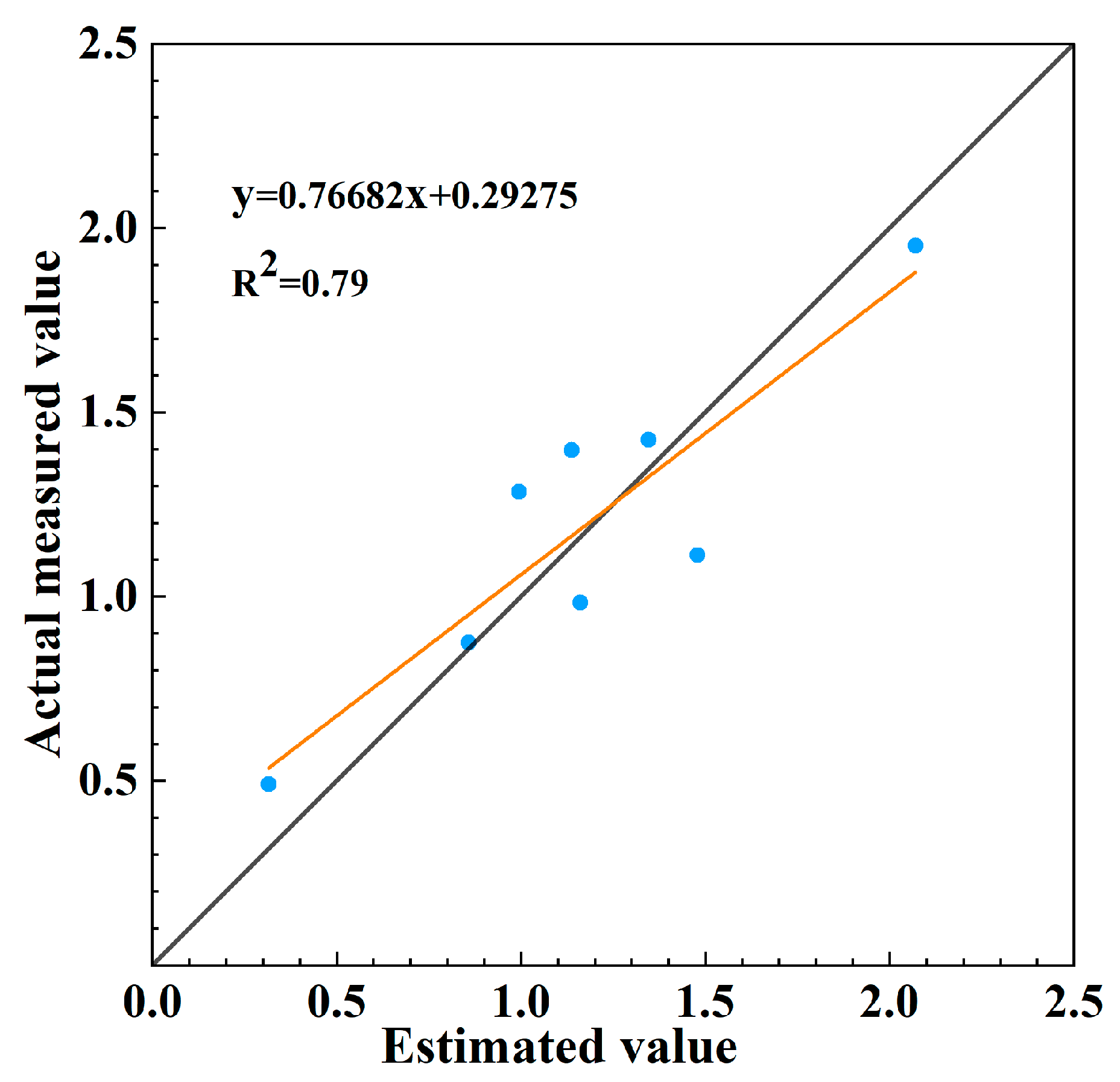
3.4. Validation of Measured Data
3.5. Applicability Test of the FMC Estimation Method
4. Discussion
4.1. Comparison of FMC Estimation Models
4.2. Impact Factor of the Model
4.2.1. Robustness Analysis
4.2.2. Effect of LAI
4.3. Indicator Potential of FMC for Forest Fires
4.4. Limitations and Future Research
4.4.1. Effect of Terrain
4.4.2. Cloud Interference
4.4.3. Limitation of Model Validation
4.4.4. Future Research
5. Conclusions
- (1)
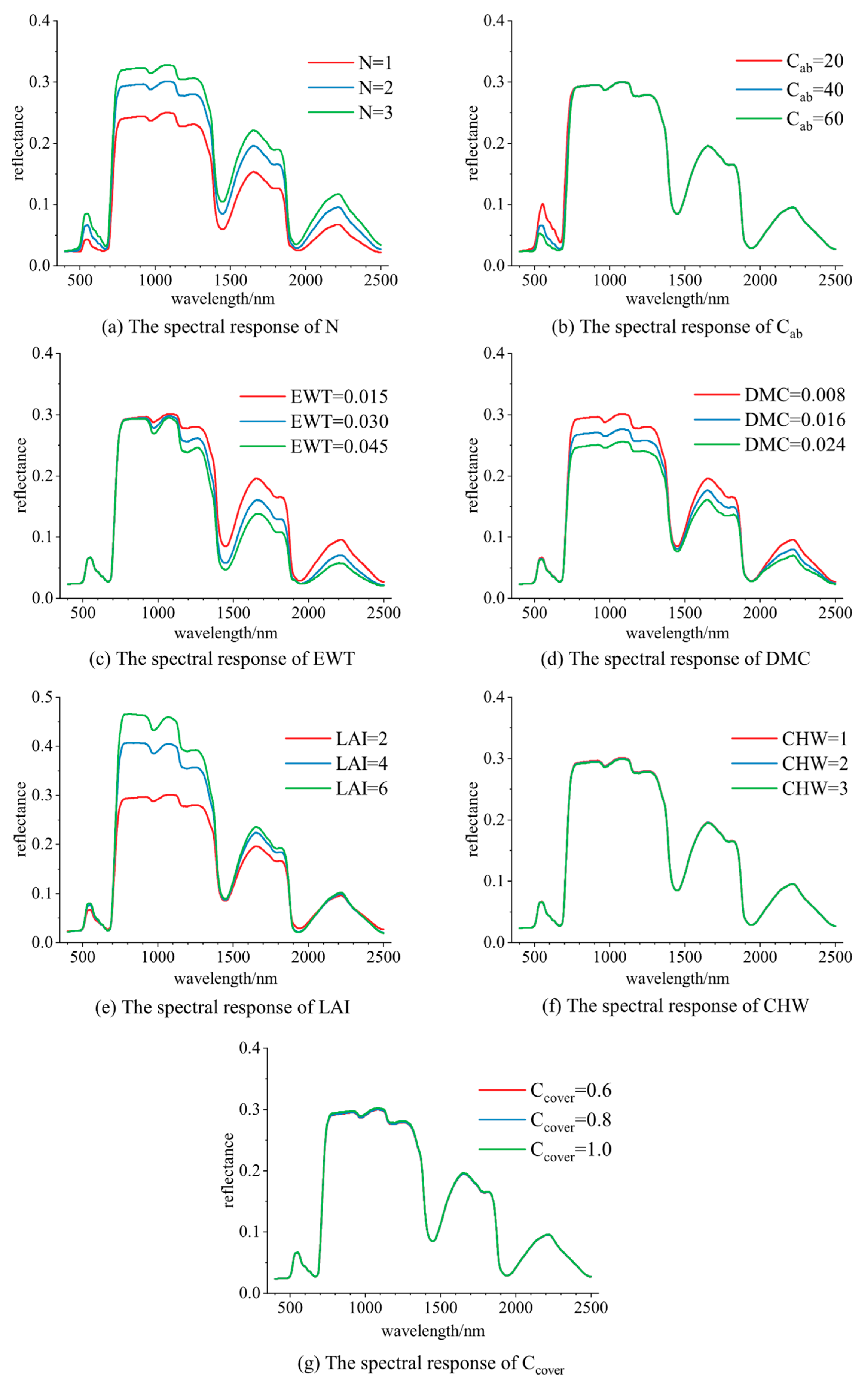
- Leaf structural parameter (N), equivalent water thickness (EWT), dry matter weight (DMC), and leaf area index (LAI) exhibited significant influence on the spectral curves generated by the two-layer coupled model employed for forward simulation. Notably, LAI had a strong impact on the 700–1450 nm and 1650 nm bands, which are particularly sensitive to vegetation water content. Consequently, it was observed that variations in LAI played a crucial role in achieving an accurate estimation of FMC.
- (2)
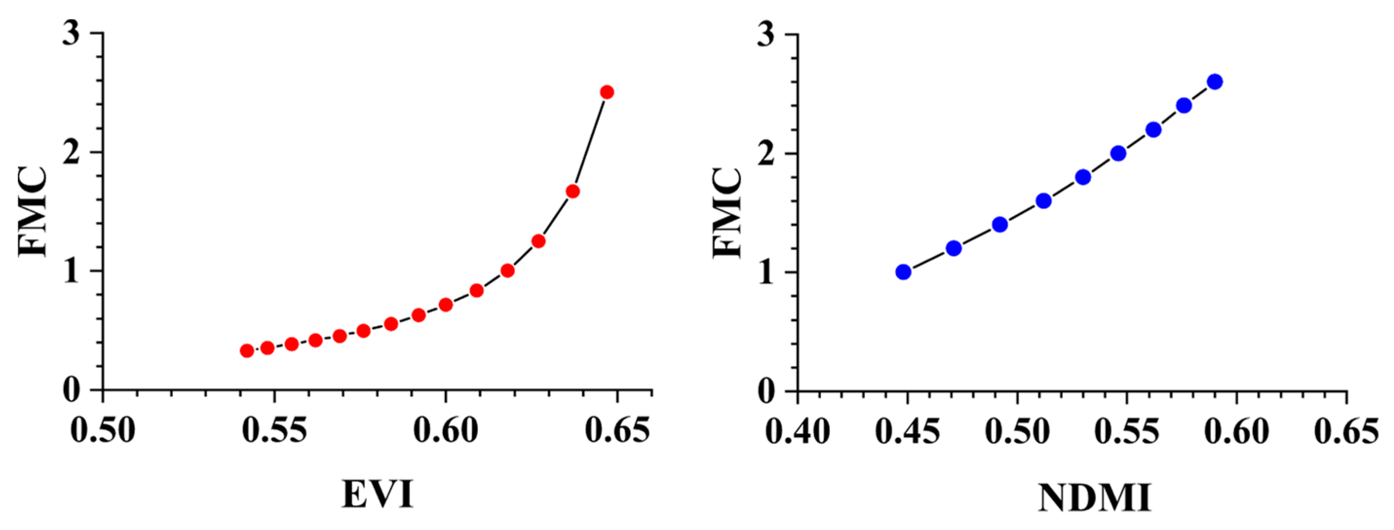
- A distinct correlation was observed when combining the vegetation index, water index, and FMC. An estimation method based on a combination of EVI–NDMI was developed to directly calculate FMC. Compared with the traditional FMC estimation model, this method eliminated errors arising from using the loss function in physical model-based forward simulations.
- (3)
- Using the estimation model, the study projected the FMC one week before the Chongqing forest fire in 2022 and identified a significant declining trend in the local FMC leading up to the fire event. This trend highlights the effectiveness of early forest fire warnings made possible by the proposed FMC estimation model.
Author Contributions
Funding
Data Availability Statement
Conflicts of Interest
References
- Szpakowski, D.; Jensen, J. A Review of the Applications of Remote Sensing in Fire Ecology. Remote Sens. 2019, 11, 2638. [Google Scholar] [CrossRef]
- Tian, X.; Shu, L. Forest Fires and Sustainable Development. World For. Res. 2003, 16, 38–41. [Google Scholar] [CrossRef]
- Guo, F.; Zhang, L.; Jin, S.; Tigabu, M.; Su, Z.; Wang, W. Modeling Anthropogenic Fire Occurrence in the Boreal Forest of China Using Logistic Regression and Random Forests. Forests 2016, 7, 250. [Google Scholar] [CrossRef]
- Pyne, S.J. Introduction to Wildland Fire. Fire Management in the United States; John Wiley & Sons: Hoboken, NJ, USA, 1984. [Google Scholar]
- Gale, M.G.; Cary, G.J.; Van Dijk, A.I.J.M.; Yebra, M. Forest fire fuel through the lens of remote sensing: Review of approaches, challenges and future directions in the remote sensing of biotic determinants of fire behaviour. Remote Sens. Environ. 2021, 255, 112282. [Google Scholar] [CrossRef]
- Arcos, M.A.; Balaguer-Beser, Á.; Ruiz, L.Á. Live fuel moisture content modeling and mapping using spectral, meteorological, and topographic data. In Proceedings of the Ninth International Conference on Remote Sensing and Geoinformation of the Environment (RSCy2023), Ayia Napa, Cyprus, 3–5 April 2023; pp. 21–29. [Google Scholar] [CrossRef]
- Hyoung, L.J. Prediction of Large-Scale Wildfires With the Canopy Stress Index Derived from Soil Moisture Active Passive. Ieee J. Sel. Top. Appl. Earth Obs. Remote Sens. 2021, 14, 2096–2102. [Google Scholar] [CrossRef]
- Przezdziecki, K.; Zawadzki, J.; Cieszewski, C.; Bettinger, P. Estimation of soil moisture across broad landscapes of Georgia and South Carolina using the triangle method applied to MODIS satellite imagery. Silva Fenn. 2017, 51, 1683. [Google Scholar] [CrossRef]
- Luo, K.; Quan, X.; He, B.; Yebra, M. Effects of Live Fuel Moisture Content on Wildfire Occurrence in Fire-Prone Regions over Southwest China. Forests 2019, 10, 887. [Google Scholar] [CrossRef]
- Cawson, J.G.; Duff, T.J.; Tolhurst, K.G.; Baillie, C.C.; Penman, T.D. Fuel moisture in Mountain Ash forests with contrasting fire histories. For. Ecol. Manag. 2017, 400, 568–577. [Google Scholar] [CrossRef]
- Li, M.; Jiao, M.; Wang, W.; Chen, R.; Fan, C. Global Live Fuel Moisture Content Dynamic Monitoring Based on Modis Data Observation. In Proceedings of the IGARSS 2023—2023 IEEE International Geoscience and Remote Sensing Symposium, Pasadena, CA, USA, 16–21 July 2023; pp. 3303–3306. [Google Scholar] [CrossRef]
- Leblon, B. Monitoring forest fire danger with remote sensing. Nat. Hazards 2005, 35, 343–359. [Google Scholar] [CrossRef]
- Saatchi, S.; Halligan, K.; Despain, D.G.; Crabtree, R.L. Estimation of forest fuel load from radar remote sensing. IEEE Trans. Geosci. Remote Sens. 2007, 45, 1726–1740. [Google Scholar] [CrossRef]
- Deng, B.; Yang, W.N.; Mu, N.; Zhang, C. The Research of Vegetation Water Content Based on Spectrum Analysis and Angle Slope Index. Spectrosc. Spectr. Anal. 2016, 36, 2546–2552. [Google Scholar]
- Tang, Y.; Wang, X.; Lu, C.; Zhao, C. Estimating the canopy water content of alfalfa based on the PROSAIL model and spectral index. J. Lanzhou Univ. Nat. Sci. 2023, 59, 55–62. [Google Scholar] [CrossRef]
- Jacquemoud, S.; Baret, F. PROSPECT: A model of leaf optical properties spectra. Remote Sens. Environ. 1990, 34, 75–91. [Google Scholar] [CrossRef]
- Kötz, B.; Schaepman, M.; Morsdorf, F.; Bowyer, P.; Itten, K.; Allgöwer, B. Radiative transfer modeling within a heterogeneous canopy for estimation of forest fire fuel properties. Remote Sens. Environ. 2004, 92, 332–344. [Google Scholar] [CrossRef]
- Jacquemoud, S. Inversion of the PROSPECT + SAIL canopy reflectance model from AVIRIS equivalent spectra: Theoretical study. Remote Sens. Environ. 1993, 44, 281–292. [Google Scholar] [CrossRef]
- Dawson, T.P.; Curran, P.J.; Plummer, S.E. LIBERTY—Modeling the effects of leaf biochemical concentration on reflectance spectra. Remote Sens. Environ. 1998, 65, 50–60. [Google Scholar] [CrossRef]
- Huemmrich, K.F. The GeoSail model: A simple addition to the SAIL model to describe discontinuous canopy reflectance. Remote Sens. Environ. 2001, 75, 423–431. [Google Scholar] [CrossRef]
- Gastelluetchegorry, J.P.; Pinel, V.; Zagolski, F.; Demarez, V. Modeling radiative transfer in heterogeneous 3D vegetation canopies. In Proceedings of the Conference on Multispectral and Microwave Sensing of Forestry, Hydrology, and Natural Resources, Rome, Italy, 26–30 September 1994; pp. 38–49. [Google Scholar] [CrossRef]
- Xie, Q.; Quan, X.; He, B. Wildfire Danger Assessment Over Southwest China Based on Short-Term Features of Weather and Fuel Variables. In Proceedings of the 2021 IEEE International Geoscience and Remote Sensing Symposium, IGARSS 2021, Brussels, Belgium, 12–16 July 2021; pp. 8648–8651. [Google Scholar] [CrossRef]
- Yu, Y.; Fan, W.; Yang, X. Comparisons of three models for vegetation canopy bi-directional reflectance distribution function. Acta Phytoecol. Sin. 2012, 36, 55–62. [Google Scholar] [CrossRef]
- Marino, E.; Yebra, M.; Guillén-Climent, M.; Algeet, N.; Tomé, J.L.; Madrigal, J.; Guijarro, M.; Hernando, C.J.R.S. Investigating live fuel moisture content estimation in fire-prone shrubland from remote sensing using empirical modelling and RTM simulations. Remote Sens. 2020, 12, 2251. [Google Scholar] [CrossRef]
- Wang, L.; Hunt, E.R.; Qu, J.J.; Hao, X.; Daughtry, C.S.T. Remote sensing of fuel moisture content from ratios of narrow-band vegetation water and dry-matter indices. Remote Sens. Environ. 2013, 129, 103–110. [Google Scholar] [CrossRef]
- Cunill Camprubí, À.; González-Moreno, P.; Resco de Dios, V.J.R.S. Live fuel moisture content mapping in the Mediterranean Basin using random forests and combining MODIS spectral and thermal data. Remote Sens. 2022, 14, 3162. [Google Scholar] [CrossRef]
- Santos, F.L.M.; Couto, F.T.; Dias, S.S.; Ribeiro, N.d.A.; Salgado, R. Vegetation fuel characterization using machine learning approach over southern Portugal. Remote Sens. Appl. Soc. Environ. 2023, 32, 101017. [Google Scholar] [CrossRef]
- Cao, Y.; Wang, M.; Liu, K. Wildfire Susceptibility Assessment in Southern China: A Comparison of Multiple Methods. Int. J. Disaster Risk Sci. 2017, 8, 164–181. [Google Scholar] [CrossRef]
- Lai, G.K.; Quan, X.W.; He, B.B. Assessment of the Effect of PROSAILH for Open and Closed Shrublands Live Fuel Moisture Content Retrieval. In Proceedings of the IEEE International Geoscience and Remote Sensing Symposium (IGARSS), Electr Network, Waikoloa, HI, USA, 26 September–2 October 2020; pp. 6778–6781. [Google Scholar] [CrossRef]
- Li, H.; Fan, W.; Yu, Y.; Yang, X. Leaf Area Index Retrieval Based on Prospect, Liberty and Geosail Models. Sci. Silvae Sin. 2011, 47, 75–81. [Google Scholar] [CrossRef]
- Quan, X.; He, B.; Liu, X.; Liao, Z.; Qiu, S.; Yin, C. Retrieval of fuel moisture content by using radiative transfer models from optical remote sensing data. J. Remote Sens. 2019, 23, 62–77. [Google Scholar] [CrossRef]
- Mo, Y.; Zhang, W.; Zhang, L. Simulation of Hyperspectral Remote Sensing Image Based on PROSAIL Model. Infrared 2016, 37, 1–7. [Google Scholar]
- Quan, X.; Li, Y.; He, B.; Cary, G.J.; Lai, G. Application of Landsat ETM+ and OLI Data for Foliage Fuel Load Monitoring Using Radiative Transfer Model and Machine Learning Method. IEEE J. Sel. Top. Appl. Earth Obs. Remote Sens. 2021, 14, 5100–5110. [Google Scholar] [CrossRef]
- Quan, X.; Xie, Q.; He, B.; Luo, K.; Liu, X. Integrating remotely sensed fuel variables into wildfire danger assessment for China. Int. J. Wildland Fire 2021, 30, 822. [Google Scholar] [CrossRef]
- Feng, X.; Zeng, Y.; Wu, Z.; Hang, W.; Wei, S.; Tang, L.; Hu, H. Remote Sensing Retrieval of FMC in Subtropical Forests of Guangdong Based on Satellite Multispectral Data. J. Univ. Electron. Sci. Technol. China 2022, 51, 432–437. [Google Scholar]
- Zhang, X.; Jiao, Z.; Zhao, C.; Yin, S.; Cui, L.; Dong, Y.; Zhang, H.; Guo, J.; Xie, R.; Li, S.; et al. Retrieval of Leaf Area Index by Linking the PROSAIL and Ross-Li BRDF Models Using MODIS BRDF Data. Remote Sens. 2021, 13, 4911. [Google Scholar] [CrossRef]
- Jiang, H.; Chai, L.; Jia, K.; Liu, J.; Yang, S.; Zheng, J. Estimation of water content for short vegetation based on PROSAIL model and vegetation water indices. J. Remote Sens. 2021, 25, 1025–1036. [Google Scholar] [CrossRef]
- Ma, J.; Huang, S.; Li, J.; Li, X.; Song, X.; Leng, P.; Sun, Y. Global Sensitivity Analysis of Parameters in the PROSAIL Model Based on Modified Sobol’s Method. Bull. Surv. Mapp. 2016, 3, 33–35. [Google Scholar] [CrossRef]
- Van Hoang, T.; Chou, T.Y.; Fang, Y.M.; Nguyen, N.T.; Nguyen, Q.H.; Xuan Canh, P.; Ngo Bao Toan, D.; Nguyen, X.L.; Meadows, M.E. Mapping Forest Fire Risk and Development of Early Warning System for NW Vietnam Using AHP and MCA/GIS Methods. Appl. Sci. 2020, 10, 4348. [Google Scholar] [CrossRef]
- Caccamo, G.; Chisholm, L.A.; Bradstock, R.A.; Puotinen, M.L. Using remotely-sensed fuel connectivity patterns as a tool for fire danger monitoring. Geophys. Res. Lett. 2012, 39, 1–5. [Google Scholar] [CrossRef]
- Raymond Hunt, E.; Wang, L.; Qu, J.J.; Hao, X. Remote sensing of fuel moisture content from canopy water indices and normalized dry matter index. J. Appl. Remote Sens. 2012, 6, 061705. [Google Scholar] [CrossRef]
- Zhang, J.; Xu, Y.; Yao, F.; Wang, P.; Guo, W.; Li, L.; Yang, L. Advances in estimation methods of vegetation water content based on optical remote sensing techniques. Sci. China Technol. Sci. 2010, 53, 1159–1167. [Google Scholar] [CrossRef]
- Quan, X.; He, B.; Yebra, M.; Yin, C.; Liao, Z.; Li, X. Retrieval of forest fuel moisture content using a coupled radiative transfer model. Environ. Model. Softw. 2017, 95, 290–302. [Google Scholar] [CrossRef]
- Bach, H.; Verhoef, W. Sensitivity studies on the effect of surface soil moisture on canopy reflectance using the radiative transfer model GeoSAIL. In Proceedings of the 23rd International Geoscience and Remote Sensing Symposium (IGARSS 2003), Toulouse, France, 21–25 July 2003; pp. 1679–1681. [Google Scholar] [CrossRef]
- Wang, L.; Niu, Z. Sensitivity of Vegetation Parameters based on PROSAIL Model. Remote Sens. Technol. Appl. 2014, 29, 219–223. [Google Scholar]
- Wang, L.; Quan, X.; He, B.; Yebra, M.; Xing, M.; Liu, X. Assessment of the Dual Polarimetric Sentinel-1A Data for Forest Fuel Moisture Content Estimation. Remote Sens. 2019, 11, 1568. [Google Scholar] [CrossRef]
- Costa-Saura, J.M.; Balaguer-Beser, A.; Ruiz, L.A.; Pardo-Pascual, J.E.; Soriano-Sancho, J.L. Empirical Models for Spatio-Temporal Live Fuel Moisture Content Estimation in Mixed Mediterranean Vegetation Areas Using Sentinel-2 Indices and Meteorological Data. Remote Sens. 2021, 13, 3726. [Google Scholar] [CrossRef]
- Wu, X.; Zhang, G.; Yang, Z.G.; Tan, S.Q.; Yang, Y.K.; Pang, Z.H. Machine Learning for Predicting Forest Fire Occurrence in Changsha: An Innovative Investigation into the Introduction of a Forest Fuel Factor. Remote Sens. 2023, 15, 4208. [Google Scholar] [CrossRef]
- Hu, G.; Li, A. BOST: A Canopy Reflectance Model Suitable for Both Continuous and Discontinuous Canopies Over Sloping Terrains. IEEE Trans. Geosci. Remote Sens. 2022, 60, 4416119. [Google Scholar] [CrossRef]
- Hu, H.; Liang, Y.; Sun, L.; Song, Y. Effects of simulated aspect and gradient of slope on moisture of combustible material in laboratory. J. For. Environ. 2016, 36, 80–85. [Google Scholar] [CrossRef]
- He, B.; Liao, Z.; Yin, C.; Quan, X.; Qiu, S.; Xing, M.; Li, X.; Bai, X.; Li, Y.; Xu, D. Theory and application status of quantitative remote sensing in cloudy and hilly regions. Dianzi Keji Daxue Xuebao/J. Univ. Electron. Sci. Technol. China 2016, 45, 533–550. [Google Scholar]
- Wang, W.; Quan, X. Estimation of Live Fuel Moisture Content From Multiple Sources of Remotely Sensed Data. IEEE Geosci. Remote Sens. Lett. 2023, 20, 3002405. [Google Scholar] [CrossRef]
- Hou, X.; Wang, M.; Liu, S.; Gao, S.; Sui, X.; Liang, S.; Wan, H. Comparsion between Prosail Model and Landsat 8 Images in Inversion of Water Content of Wheat Canopy. J. Triticeae Crops 2018, 38, 493–497. [Google Scholar]


| Model Type | Model | Merit | Demerit |
|---|---|---|---|
| Empirical model | Spectral model | High accuracy in estimating FMC. | Needs a large number of measured data; existence of regional limitations. |
| Physical model | PROSAIL | Can be approximated by estimating EWT and DMC; high accuracy in estimating FMC for uniformly distributed vegetation. | Only suitable for vegetation with uniform canopy distribution; has hot spot effect. |
| Liberty | Suitable for coniferous forests. | Lack of dry matter weight parameter; can only be approximated by other parameters. | |
| GEOSAIL | Suitable for reflectance simulation of heterogeneous canopy. | Has hot spot effect. | |
| DART | Three-dimensional model; the light transmission process of forest canopy can be well restored. | Large amount of calculation. |
| Sample Plot Number | Longitude | Latitude | Land Cover Type |
|---|---|---|---|
| 1 | 100°12′3″ E | 25°34′57″ N | Forest |
| 2 | 100°10′1″ E | 25°38′39″ N | Forest |
| 3 | 100°8′9″ E | 25°41′52″ N | Forest |
| 4 | 100°6′39″ E | 25°45′10″ N | Forest |
| 5 | 100°6′21″ E | 25°49′13″ N | Grass |
| 6 | 100°5′19″ E | 25°53′19″ N | Forest |
| 7 | 100°13′51″ E | 25°33′3″ N | Forest |
| 8 | 100°11′14″ E | 25°42′12″ N | Cropland |
| Model | Input Parameter | Symbol | Unit | Value |
|---|---|---|---|---|
| PROSPECT (Lower plants) | Leaf structural parameters | N | / | 2 |
| Chlorophyll content | Cab | μg·cm−2 | 40 | |
| Carotenoid content | Car | μg·cm−2 | 8 | |
| Brown pigment fraction | Cbrown | / | 0 | |
| Equivalent water thickness | EWT | g·cm−2 | 0.015 | |
| Dry matter weight | DMC | g·cm−2 | 0.008 | |
| SAIL (Lower plants) | Solar zenith angle | tts | (°) | 30 |
| Observed zenith angle | tto | (°) | 0 | |
| Leaf area index | LAI | / | 2 | |
| Leaf inclination distribution function | LIDFa | / | −0.35 | |
| LIDFb | / | −0.15 | ||
| Hot spot effect factor | hspot | / | 0.02 | |
| Soil reflectance | Rsoil | / | 0.47 | |
| PROSPECT (Upper forest) | Leaf structural parameters | N | / | 2 |
| Chlorophyll content | Cab | μg·cm−2 | 40 | |
| Carotenoid content | Car | μg·cm−2 | 8 | |
| Brown pigment fraction | Cbrown | / | 0 | |
| Equivalent water thickness | EWT | g·cm−2 | 0.005–0.02 | |
| Dry matter weight | DMC | g·cm−2 | 0.001–0.015 | |
| GEOSAIL (Upper forest) | Solar zenith angle | tts | (°) | 30 |
| Observed zenith angle | tto | (°) | 0 | |
| Leaf area index | LAI | / | 0–6 | |
| Leaf inclination distribution function | LIDFa | / | −0.35 | |
| LIDFb | / | −0.15 | ||
| Canopy cover | Ccover | / | 0.85 | |
| Canopy height-to-width ratio | CHW | / | 2 | |
| Crown shape | / | / | Cone | |
| Hot spot effect factor | hspot | / | 0.02 | |
| Soil reflectance | Rsoil | / | Lower plants’ reflectance |
| Input Parameter | Symbol | Unit | Base Value |
|---|---|---|---|
| Leaf structural parameters | N | / | 2 |
| Chlorophyll content | Cab | μg·cm−2 | 40 |
| Carotenoid content | Car | μg·cm−2 | 8 |
| Brown pigment fraction | Cbrown | / | 0 |
| Equivalent water thickness | EWT | g·cm−2 | 0.015 |
| Dry matter weight | DMC | g·cm−2 | 0.008 |
| Solar zenith angle | tts | (°) | 30 |
| Observed zenith angle | tto | (°) | 0 |
| Leaf area index | LAI | / | 2 |
| Leaf inclination distribution function | LIDFa | / | −0.35 |
| LIDFb | / | −0.15 | |
| Hot spot effect factor | hspot | / | 0.02 |
| Soil reflectance | Rsoil | / | 0.47 |
| LAI | a1 | a2 | a3 | a4 | a5 |
|---|---|---|---|---|---|
| 0.1 | 3069.379 | −846.395 | 58.362 | −0.634 | 0.154 |
| 0.12 | 996.128 | −285.384 | 20.446 | −0.219 | 0.057 |
| 0.14 | 1587.222 | −470.94 | 34.943 | −0.401 | 0.109 |
| 0.16 | 1365.025 | −418.881 | 32.146 | −0.435 | 0.124 |
| 0.18 | 1104.593 | −349.556 | 27.667 | −0.412 | 0.123 |
| 0.2 | 1073.114 | −351.119 | 28.733 | −0.377 | 0.118 |
| 0.23 | 1063.039 | −363.702 | 31.124 | −0.43 | 0.142 |
| 0.26 | 946.679 | −337.517 | 30.102 | −0.446 | 0.156 |
| 0.3 | 831.378 | −312.011 | 29.293 | −0.465 | 0.171 |
| 0.35 | 668.267 | −266.844 | 26.66 | −0.42 | 0.167 |
| 0.4 | 695.166 | −293.326 | 30.97 | −0.513 | 0.214 |
| 0.45 | 553.187 | −245.027 | 27.162 | −0.517 | 0.226 |
| 0.5 | 449.88 | −208.998 | 24.301 | −0.474 | 0.217 |
| 0.55 | 459.904 | −223.352 | 27.153 | −0.538 | 0.257 |
| 0.6 | 358.562 | −181.497 | 22.999 | −0.468 | 0.230 |
| 0.7 | 350.395 | −190.789 | 26.013 | −0.593 | 0.309 |
| 0.8 | 359.677 | −209.316 | 30.509 | −0.739 | 0.403 |
| 0.9 | 266.166 | −164.52 | 25.473 | −0.634 | 0.36 |
| 1.1 | 246.09 | −168.358 | 28.862 | −0.802 | 0.484 |
| 1.3 | 218.468 | −162.609 | 30.342 | −0.926 | 0.588 |
| 1.6 | 158.4 | −130.511 | 26.976 | −0.973 | 0.652 |
| 2.1 | 15.362 | −14.354 | 3.369 | −0.156 | 0.111 |
| 2.6 | 13.508 | −13.804 | 3.584 | −0.209 | 0.154 |
| 3.0 | 14.264 | −15.376 | 4.175 | −0.297 | 0.224 |
| 4.0 | 2.726 | −3.213 | 0.958 | −0.104 | 0.081 |
| 6.0 | 3.074 | −3.91 | 1.271 | −0.268 | 0.213 |
Disclaimer/Publisher’s Note: The statements, opinions and data contained in all publications are solely those of the individual author(s) and contributor(s) and not of MDPI and/or the editor(s). MDPI and/or the editor(s) disclaim responsibility for any injury to people or property resulting from any ideas, methods, instructions or products referred to in the content. |
© 2024 by the authors. Licensee MDPI, Basel, Switzerland. This article is an open access article distributed under the terms and conditions of the Creative Commons Attribution (CC BY) license (https://creativecommons.org/licenses/by/4.0/).
Share and Cite
Yang, K.; Tang, B.-H.; Fu, W.; Zhou, W.; Fu, Z.; Fan, D. Estimation of Forest Canopy Fuel Moisture Content in Dali Prefecture by Combining Vegetation Indices and Canopy Radiative Transfer Models from MODIS Data. Forests 2024, 15, 614. https://doi.org/10.3390/f15040614
Yang K, Tang B-H, Fu W, Zhou W, Fu Z, Fan D. Estimation of Forest Canopy Fuel Moisture Content in Dali Prefecture by Combining Vegetation Indices and Canopy Radiative Transfer Models from MODIS Data. Forests. 2024; 15(4):614. https://doi.org/10.3390/f15040614
Chicago/Turabian StyleYang, Kun, Bo-Hui Tang, Wei Fu, Wei Zhou, Zhitao Fu, and Dong Fan. 2024. "Estimation of Forest Canopy Fuel Moisture Content in Dali Prefecture by Combining Vegetation Indices and Canopy Radiative Transfer Models from MODIS Data" Forests 15, no. 4: 614. https://doi.org/10.3390/f15040614
APA StyleYang, K., Tang, B.-H., Fu, W., Zhou, W., Fu, Z., & Fan, D. (2024). Estimation of Forest Canopy Fuel Moisture Content in Dali Prefecture by Combining Vegetation Indices and Canopy Radiative Transfer Models from MODIS Data. Forests, 15(4), 614. https://doi.org/10.3390/f15040614