Abstract
Forest and its dynamics are of great significance for accurately estimating regional carbon sequestration, emissions and carbon sink capacity. In this work, an efficient framework that integrates remote sensing, deep learning and statistical modeling was proposed to extract forest change information and then derive forest carbon storage dynamics during the period 2017 to 2020 in Jiangning District, Nanjing, Eastern China. Firstly, the panchromatic band and multi-spectral bands of GF-1 images were fused by using four different methods; Secondly, an improved Mask-RCNN integrated with Swin Transformer was devised to extract forest distribution information in 2020. Finally, by using the substitution strategy of space for time in the 2017 Forest Management and Planning Inventory (FMPI) data, local carbon density allometric growth equations were fitted by coniferous forest and broad-leaved forest types and compared, and the optimal fitting was accordingly determined, followed by the measurements of forest-change-induced carbon storage dynamics. The results indicated that the improved Mask-RCNN synergizing with the Swin Transformer gained an overall accuracy of 93.9% when mapping the local forest types. The carbon storage of forest standing woods was calculated at 1,449,400 tons in 2020, increased by 14.59% relative to that of 2017. This analysis provides a technical reference for monitoring forest change and lays a data foundation for local agencies to formulate forest management policies in the process of achieving dual-carbon goals.
1. Introduction
As the largest organic “carbon pool” in terrestrial ecosystems, forest provides about 80% of the global above-ground vegetation biomass [1], and its carbon storage approximately accounts for 46.6% of the terrestrial ecosystems’ carbon stock [2]. Thus, widespread forest dynamics inevitably alters the carbon sequestration capability of forest ecosystems and then promotes global climate change and the greenhouse effect [3]. Therefore, accurate acquisition of forest dynamics information contributes to evaluating the carbon sink potential of forest ecosystems in the near future, which lays an underlying data basis for assessing the degree of achieving the dual-carbon goals in China [4].
The traditional means for capturing forest dynamics information mainly rely on massive in situ surveys. However, this manner has the drawbacks of high time and labor costs, poor timeliness and potential low accessibility, therefore making it difficult to meet the needs of dynamic monitoring over wide forested regions [5,6]. Fortunately, the emergence and advancement of remote sensing technology have overcome the defects of the traditional survey means. In particular, high-spatiotemporal-resolution remote sensing data contain more structural details and spectral and phenological variations; although such an analysis process tends to be more complex, it is more conducive to the fine identification and mapping of forest types and even tree species [7,8]. In recent decades, pixel-based classification methods have been widely used in forest information extraction based on medium- or high-resolution imagery. For example, Huang et al. combined Sentinel-2 spectral features and radar data backscattering features to classify tree species of typical plantation forests in the tropics via the random forest method [9]. Although the classical statistics-based or machine learning methods have operational speed and simplicity, the “salt and pepper phenomenon” is quite common in classification results [10]. To minimize the negative effects of pixel-based analysis methods, Object-based Image Analysis (OBIA) has been proposed and applied in forest-related remote sensing efforts because it can make full use of shallow information such as spectral, texture and geometric features and the spatial topology of features in medium- or high-resolution remote sensing imagery for classification [11]. For example, Mao et al. combined Sentinel active and passive remote sensing data to develop an object-oriented SNIC+RF algorithm to classify the land cover of Qianjiangyuan National Park, obtaining an overall accuracy of 93.98% [12]. However, OBIA only considers the shallow features within the segmented objects; it is prone to cause mis-segmentation and misclassification in complex situations [13]. Therefore, determining how to adequately extract and utilize effective information from medium- or high-resolution remote sensing images becomes the key to improving classification accuracy.
Along with the escalation in computer processing power, there has been a fast development of deep learning in a wide range of application areas [14]. Deep learning methods are representation learning methods with multiple levels of representation, obtained by composing simple but non-linear modules that each transform the representation at one level (starting with the raw input) into a representation at a higher, slightly more abstract level. Deep learning extends standard machine learning by discovering intermediate representations that can be used to solve more complex problems [15]. Convolutional neural networks (CNNs), first proposed by Yann LeCun for image processing, are some of the most widely used deep neural networks currently [16]. CNNs and their derived network models, such as the fully convolutional networks (FCNs), U-net and DeepLab V+, have been widely used in high-resolution image classification, and they have shown their robustness and strong generalization ability as well as the capability of extracting and utilizing high-level features from remote sensing images [17]. In addition, CNN-based model improvements continue to confirm these observed advantages. For example, He et al. combined the features of urban objects in high-resolution images and the characteristics of urban forest itself and proposed the Object-Based U-Net-Dense Net-Coupled Network (OUDN) based on a CNN for extracting urban forests, and its extraction accuracy reached 0.997 [18].
In particular, the Mask-Region Convolutional Neural Network (Mask-RCNN) model is a flexible and generalized instance segmentation framework [19] that is commonly used for target recognition and extraction [20,21]. Based on this, Xie et al. proposed a Modified Mask-RCNN model for urban forest extraction after hyperpixel segmentation of GF-2 images and transferred the model to UAV image classification, achieving a high overall accuracy of 92.48% [22]. Shi et al. also applied the Modified Mask-RCNN model to extract urban–suburban fragmented land cover types from several types of high-resolution satellite images in Nanjing, and its accuracy was higher than that of the object-oriented decision-tree-based classification model [23]. However, due to the limited receptive field of the model structure, Mask-RCNN produced a fuzzy target edge segmentation and missed small targets [24,25]. In contrast, the Transformer technology builds a global information model by capturing long-distance dependencies of the entire feature graph with an attention mechanism [26,27]. In particular, the Swin Transformer model, an improved version of Transformer, has global modeling capability, and its hierarchical network structure and sliding window information interaction mode expand the receptive field to some extent to reduce the amount of computation, making it more suitable for multi-scale target classification recognition and extraction [28]. For example, Gao et al. used an instance segmentation optimization method by incorporating Swin Transformer to effectively solve the problem of difficult segmentation for multi-larval individual image recognition in complex real-world scenes, and they achieved a satisfactory result [29]. Although these existing deep learning models have had different levels of success in extracting and recognizing objects of interest from remote sensing images, coupling Mask-RCNN with Swin Transformer to accurately identify different forest types including coniferous forest, broad-leaved forest and shrub forest from 2 m resolution satellite images has been rarely attempted, and it deserves further investments and tests.
A forest growth model is an important tool for studying tree growth and stand harvests; it helps to conceptualize and abstract the complex phenomenon and process of tree growth and to simulate and predict tree change and future development trends [30]. The whole stand model is a kind of stand growth and harvest model with nearly a hundred years of history; it describes the total amount of the whole stand and the growth process of average individual trees [31]. According to whether the density factor is introduced into the model as an independent variable, the whole stand model can be divided into two categories. One is the density-independent model, an example of a model belonging to this category is the traditional stand harvest table in Europe and America, with little practical significance. Another type of model is the density-related model, which takes the index of stand density as an independent variable to simulate the change in stand growth or harvest. Such models are widely used at present [32]. For example, the Gompertz model is often used to describe the growth of certain plants and the law of economic activities [33]. Zhao et al. applied the Gompertz growth model to predict the output value of forest products; the relative error was only 0.0082%, and the correlation coefficient reached 0.9992 [34]. The Richards model has been widely used in various fields of forest growth, and it has the advantages of an accurate description of the growth process and the strongest applicability [35]. For example, by taking stand age, site index and stand density index as independent variables, Jiang et al. studied the whole stand model of a Chinese fir plantation with variable density based on the Richards model, achieving a high accuracy of 82.48% [36]. Based on the Richards model, Feng et al. established a full-stand model of Beijing’s Platyphelus orientales plantation based on the compatibility of the harvest model and showed a strong applicability [37]. Wang et al. used the logistic model to study the population quantitative characteristics of Taxus chinensis, a rare and endangered plant, and fitted the S-shaped curve of population growth, with a fitting accuracy of more than 90% [38]. Overall, the density-related whole stand models are simple to understand and easy to use, and they can directly predict the growth and harvest of the stand per unit area; thus, the total harvest of the whole stand can be easily derived. With the introduction of new statistical methods, such as the mixed-effect model, machine learning and quantile regression, their estimation accuracy and application range can be further improved [39]. For example, Zhang et al. studied a model of Poplus spp. and analyzed the distribution characteristics under different classes of environmental indicators based on the KNN model and RF model, and a high accuracy and good fitting effect were accordingly achieved [40]. However, the model simulation coefficients of the above-mentioned density-dependent models are species-dependent and site-specific; thus, to better predict the growth of particular stands by using these models, it is necessary to make the model parameters localized.
The estimation methods of vegetation carbon storage are mainly divided into three types [41]: (1) The first is survey-based estimation, namely estimation using regional forest survey data, and this method usually gives the most accurate results but with extremely high labor and time costs [42]. (2) The second is remote-sensing-based estimation, for which commonly used data include optical remote sensing data, LiDAR data and synthetic aperture radar (SAR) satellite data [43]. For instance, Vincent et al. used WorldView-2 and LiDAR data to perform a fine estimation of vegetation carbon storage in Auckland, New Zealand, and the accuracy reached up to 95.9% [44]. LiDAR can effectively and accurately measure tree height and three-dimensional spatial structure to derive a very high carbon estimate for individual trees or forest stands, but it is often subjected to the limitation of high operational cost [45]. Vatandaşlar et al. used SAR data to estimate the carbon stocks of Mediterranean forests, and the conclusion fully proved that the total carbon stocks of forest ecosystems could be estimated using appropriate SAR images and could be applied to forestry with good accuracy [46]. (3) The third is process-based estimation, which mainly refers to mechanism modeling. The mechanism modeling method can estimate forest carbon storage and quantitatively describe the forest carbon cycle process, but it needs a lot of parameters or variables to drive the process model, and in the reality of model application, these parameters are frequently difficult to obtain in an accurate manner [47].
The major aim of this study was to propose a forest change analysis framework that integrates deep learning and forest stand growth modeling to accurately assess the carbon storage dynamics at a district or county scale. Specifically, the deep learning Mask-RCNN model was improved by replacing ResNet101 with Swin Transformer for the accurate extraction of forest types first, and then the optimal stand carbon density growth equation was determined to accurately calculate forest growth, jointly supporting the evaluation of forest carbon storage dynamics during the period 2017–2020.
2. Materials and Methods
2.1. Study Area
The study area is located in Jiangning District, Nanjing City, Jiangsu Province (118°28′ E~119°06′ E, 31°37′ N~32°07′ N) (Figure 1). Jiangning District belongs to the northern subtropical monsoon climate zone, with an average annual temperature of 15.7 °C and an average annual precipitation of 1072.9 mm. The area contains a variety of landforms, including low hills, highlands, plains and basins. The terrain is high in the north and south and low in the center. The area is rich in water systems, with two major water systems, the Yangtze River and the Qinhuai River, and many small rivers and reservoirs are scattered throughout the area. Figure 1 shows the location of the study area and its vegetation cover. During the past few decades, Jiangning District had rapid economic development and an intense change in land use. Thus, Jiangning’s forest was frequently disturbed by human activities. Choosing Jiangning District as a study area can test the reliability and effectiveness of the proposed framework when quantifying the dynamic changes of forest carbon stocks under rapid changes, to provide a reference and data support for local forest change monitoring [48].
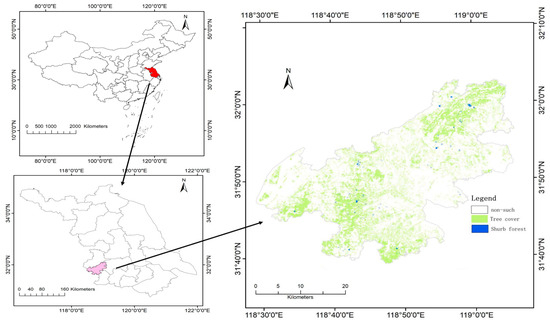
Figure 1.
Geographical location and its vegetation cover of the study area (Upper Left: the map of China’s territory; Lower Left: the map of the administrative boundaries of Jiangsu Province; Right: the 2022 vegetation cover map of the study area).
2.2. Data
In this study, two GF-1 images including a panchromatic and 4 multi-spectral (PMS) bands, acquired on 17 August and 5 September 2020, respectively, were collected and mosaicked to cover the entire study area of Jiangning District, and the images were fused and acted as the major input for subsequent fine land cover classification. The PMS camera of the GF-1 satellite provides a 2 m resolution panchromatic band and 4 8 m spatial resolution multi-spectral bands (red, green, blue and near-infrared) simultaneously. The camera has a high radiometric resolution, with a quantification level of 10 bits, and its image swath is 60 km. Additionally, a DEM with a spatial resolution of 12.5 m covering the entire study area was compiled from the Beijing KOSMOS Image Mall (a satellite image vendor) to support subsequent land cover classifications. In addition, the 2017 Forest Management and Planning Inventory (FMPI) data were collected from the Nanjing Greening and Gardening Bureau. These data were acquired by a complete field survey of all forest stands involved. Before implementing this survey, all forest stands must be delineated from current aerial photographs or large-scale topographic maps by visual interpretation, followed by deploying well-trained experienced investigators to each forest stand to capture forest stand information including tree species composition, dominant tree species, age, average height, average DBH, crown closure and disturbance type and severity. Finally, the inventory results were subjected to a quality check by limited sample plot measurements and cross-comparison. According to the needs of forest classification in the study area, the vector data of 2017 were converted into raster data. The 2017 FMPI data were used as the benchmark of forest status for the dynamic assessment. All the spatial data mentioned here were resampled to 2 m resolution to facilitate the change analysis.
2.3. Image Fusion
The post-atmospheric correction panchromatic band and multi-spectral bands of GF-1 images were fused to generate new higher-quality images with a 2 m spatial resolution by using the Brovey transform, GS transform, NND transform and wavelet transform fusion algorithms. The Brovey transform method multiplies multi-spectral images and panchromatic high-resolution images on the basis of normalization to enhance image information [49,50]; GS transform eliminates the strong correlation between the bands and reduces the redundant information by orthogonalizing the image data [51,52]; the NNDiffuse transform method can significantly improve the image processing quality and speed, and the fused images will be better when all the multi-spectral bands are covered by the panchromatic wavelength and the wavelengths of the multi-spectral bands do not overlap [53]. Wavelet transform first decomposes the panchromatic band into four new images (approximation, horizontal details, vertical details and diagonal details) and then resamples the multi-spectral bands to make their spatial resolution consistent with that of the panchromatic band; on this basis, a principal component analysis of the these resampled multi-spectral bands is implemented, followed by a histogram-matching operation between the approximation image and the first principal component image. Once this is completed, the substitution of the approximation image with the histogram-matched first principal component image and the implementation of a wavelet reconstruction analysis are conducted to obtain the fused new images [54,55]. These fusion algorithms were implemented in ENVI and Matlab packages. The evaluation of the final fused image quality is an extremely important step in the process of image fusion [56]. Generally, the evaluation includes the intuitive subjective qualitative evaluation by human visual observation and the objective quantitative evaluation by calculating quantitative statistical indicators [57,58]. The quantitative assessment indicators used in this analysis were the mean standard deviation, the mean correlation coefficient and the mean gradient [59,60].
2.4. Forest Distribution Extraction Modeling and Validation
First, because water can absorb a lot of solar energy, the reflectance of water is much lower than that of most ground objects, and its reflectance decreases with the increase in wavelength in the visible–shortwave infrared range. The normalized difference water index (NDWI) widens the reflectance gap between the near-infrared band with the weakest reflectance and the green band with the strongest reflectance for a water body through the calculation of a ratio, making the water object information more prominent [61]. In the analysis, NDWI was therefore used to classify the image into water body and non-water body classes by specifying a threshold of 0.2. Green vegetation strongly absorbs red light and strongly reflects near-infrared waves; on this basis, the normalized vegetation index (NDVI), defined as the ratio between the difference and the sum of the reflectance of the near-infrared channel and the reflectance of the visible channel, was used to highlight the signal of vegetation. NDVI can reflect vegetation coverage and growth status and can effectively remove some radiation errors. In an area covered by vegetation, the NDVI value is positive, and with the increase in vegetation coverage, the NDVI value will be increased, but it is easily saturated in high-vegetation-coverage areas [62]. Hence, NDVI was used to classify the non-water body region of the GF-1 image into vegetation areas and non-vegetation areas. In the vegetation areas, combined with the actual situation of the study area, five major land cover types, namely coniferous forests, broad-leaved forests, shrub forests, grassland and cropland, were identified as the scheme of classification. And 600 forest samples, 200 grassland samples and 200 cropland samples were picked up from the fused GF-1 false-color composite based on our local knowledge to train the classification models. Due to the complex structures of different forest types, it is difficult to accurately characterize their differences in a single remote sensing band. Therefore, we used the original multi-spectral reflectance bands [63], NDVI, Gray-Level Co-occurrence Matrix-based textural measures [64], and topographic variables including elevation, slope and aspect [65] as the inputs for the classifications of machine learning algorithms. Specifically, support vector machine (SVM), random forest (RF), Mask-RCNN and Mask-RCNN integrated with Swin Transformer were compared in terms of the classification performance. Among them, SVM is a linear classifier with the largest interval defined on the feature space, and there are several types of kernel functions available to potentially optimize the algorithm performance. For example, the Gaussian kernel function can map finite-dimensional data to a higher-dimensional space, which may give SVM a high accuracy in image classification [66]. In this study, the Gaussian kernel function was selected to extract forest types based on the SVM algorithm, with the C parameter set to 1 and the gamma parameter set to 0.1. RF is a data-driven non-parametric classification algorithm. The major parameters including the number of variables m and the number of trees T in the algorithm need to be adjusted according to specific application scenarios. In this analysis, parameters T = 100 and m = 5 were set after multiple tries. Further, ResNet101 was adopted as the backbone network part of the image feature extraction network model. Then, the sliding window of the region of interest (ROI) corresponding to the candidate frame was generated to obtain a feature map with a high-quality candidate frame, which was used for subsequent target frame location, mask recognition and image classification. The network structure consisted of the backbone feature extraction network, Region Proposal Network (RPN) and classification structure. The main feature extraction part included the Swin Transformer and the Feature Pyramid Network (FPN), which can extract features from input images and obtain feature maps with multi-scale semantic information. The proposed ROI network was mainly composed of a CNN for realizing the segmentation so as to screen the approximate candidate box of the target location. The classification structure mainly consisted of two parts: category branch and mask branch. Figure 2 displays the integrated framework that combines Mask-RCNN with Swin Transformer, which was used to extract forest distribution information.
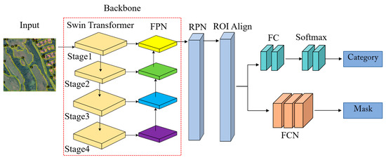
Figure 2.
The integrated framework that combines Mask-RCNN with Swin Transformer for forest type extraction.
The Mask-RCNN model combined with Swin Transformer obtained internal parameters through iterative training. After multiple experimental tests, the learning rate was set to 0.005, the training batch size was 4, and 100 iterations were performed in the training phase. To implement the classifications using the deep learning algorithms, a sample library was established according to the actual situation of the study area. The fused GF-1 false-color composite was first cut into 780 × 780 image blocks in TensorFlow (https://www.tensorflow.org/). In order to ensure the consistency and full calculation of the number of each type as far as possible, sample images with uniform distribution and complete types were selected for annotation. The sample images were rotated and flipped to increase the number of available sample images. In total, this study used 864 labeled training map sheets and 432 labeled validation map sheets. The online annotation tool VIA (VGG Image Annotator, version 2) was used to annotate the training and validation datasets (sample images); VIA is an open-source image annotation software developed by the Visual Geometry Group, does not need to be downloaded and installed, can run offline in the browser, is simple to use and can annotate points, lines and polygons.
2.5. Calculation of Forest Carbon Storage Benchmark in 2017
In the current analysis, considering the availability of data and the operability, economy and accuracy of the used methods, we only measured or calculated the carbon storage of forest living woods, excluding the carbon storage of forest soil, litter and debris, dead wood and understory shrubs and herbs. For the measurement of forest living wood carbon storage based on the 2017 FMPI data, the forest biomass conversion factor method was adopted. This method has been widely used in the estimation of forest biomass and carbon storage in wide regions because there is a good regression relationship between forest stock volume, forest biomass and carbon storage by dominant tree species, and the estimation of forest carbon storage via forest biomass has a high accuracy [67]. Thus, the carbon storage of each forest stand in Jiangning District was calculated by using Equation (1), while the carbon storage of shrub forest was calculated by using Equation (2). To minimize the calculation complexity of shrub forests, we did not differentiate tree species of shrub forests, and we just focused on different average biomass density values of shrub forests at the two time points. The parameters involved in the calculation processes for tree species are summarized in Table A1 in Appendix A. Since the parameters of BEF (biomass expansion factor), wood basic density, carbon content and root-to-stem ratio of some minor tree species were unavailable in the study area, the parameters of similar tree species from the same family or genus were used for an approximate calculation. Finally, we summed the measurements of all the forest stands of living woods and shrub forest to obtain the total carbon storage benchmark in 2017.
where Cz is the total carbon storage of forest stands (tons of carbon); Aij is the area of the jth forest stand with dominant tree species i (hm2); Vij is the stock volume per unit area of the jth forest stand with dominant tree species i (m3/hm2); BCEFij = BEFij·Di; BEFij is the biomass expansion factor of tree species i in climatic zone j, which is the ratio of above-ground biomass over the biomass of tree trunks; Rij is the ratio of root over stem of tree species i in climatic zone j; CFij is the carbon content of tree species i in climatic zone j (ton carbon/ton dry matter; C/t d.m); Mi is shrub layer biomass per unit area (hm2); Ai is shrub layer area (hm2); CFD is carbon content ratio (C/t d.m).
2.6. Derivation of the 2020 Forest Carbon Storage
Based on the outcomes of Section 2.4, we could easily obtain the spatial distributions of conventional forest stands (e.g., coniferous forest and broad-leaved forest) and the shrub forest type. For the shrub forest, we used Equation (2) to calculate the carbon storage in 2020 by specifying its newly updated biomass density per unit area, derived from limited harvesting measurements of shrubs, and its distribution area. For the conventional forest stands, their calculation of the 2020 carbon storage was divided into two parts, including the persisting forest part (pixels that were forest type in both 2017 and 2020), forest gain part (pixels that were non-forest type in 2017 but were forest in 2020). The 2020 carbon storage measurement of the persisting forest was based on the optimal local carbon density growth allometric equations. Based on the 2017 FMPI data in Nanjing, we fit the carbon density growth equations including the logistic (Equation (3)), Richards (Equation (4)) and Gompertz (Equation (5)) growth models (carbon density against forest age) of the coniferous forests and broad-leaved forests in Nanjing City by adopting the space for time substitution strategy in consideration of the availability of the inventory data of different tree species with different stand ages via RStudio package, and we selected the optimal equations for calculating the carbon storage of the persisting forests in Jiangning by specifying a 3-year growth duration in the optimal equations. For the part of forest gain, its initial forest age was set to 1.5 years (residing in the nursery with an average duration of 1.5 years for this mid-latitude region with good hydrothermal conditions); similarly, the growth duration was also set to 3 years to calculate the carbon storage by following the optimal equations for different forest types.
where y represents the carbon density of the forest stand; t represents the average age of the forest stand; and a, b and c are the model parameters to be solved.
2.7. Validation Strategies
For the validation of forest type classification, we identified another set of validation samples with the same size of 1000 pixels as the training set to construct confusion matrices. The validation sample points were selected by stratified random sampling to ensure an unbiased estimate of accuracy; 400 random points were generated in the non-forest region, and 600 random points were generated in the forest region. Then, the actual type attributes of these points were visually interpreted based on the fused GF-1 false-color composite coupled with our local knowledge. On this basis, the overall accuracy (OA) and Kappa coefficient were calculated to evaluate the classification accuracy. The formula for calculating the Kappa coefficient is written in Equation (6):
Here, Po is the overall accuracy of classification, which refers to the probability that the classification results are consistent with the true reference data, and is calculated by dividing the amount of correctly classified pixels by the total of the pixels involved in the validation. Pe is the estimate of the chance agreement, which refers to the completely random assignment of pixels to classes (e.g., dicing to determine the class of a pixel). Thus, the Kappa coefficient indicates the difference degree between the actual classifications made by a classifier and the random classifications made by chance. When the Kappa coefficient value ranges from 0.61 to 0.80, there is a substantial difference between the results of an automated classifier and the results of a random chance classifier, suggesting an indication of good classification performance. When the Kappa value ranges from 0.81 to 1.00, there is an almost perfect difference between the results of an automated classifier and the results of a random chance classifier, showing an indication of excellent classification performance.
For the validation of the fitted carbon density growth models based on the 2017 FMPI data, we collected similar research studies (Table A7 in Appendix A) and cross-compared our simulated carbon density results of coniferous forest and broad-leaved forest with the results of those similar studies to prove the effectiveness and reliability of our simulated carbon density growth models.
Figure 3 shows the overall flow chart of this study.
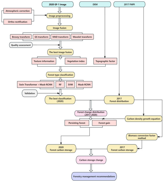
Figure 3.
The flow chart of the current analysis.
3. Results
3.1. Image Fusion
Table A2 in the Appendix lists the objective evaluation statistics of the four image fusion methods. It was found that the GS fusion method achieved the highest mean correlation coefficient, mean gradient and information entropy values, 0.9743, 63.2020 and 7.6548, respectively, and the db2 (mother wavelet)-based wavelet transform fusion method achieved the worst fusion performance, evidenced by the lowest correlation coefficient, mean gradient and information entropy values, 0.9081, 1.1443 and 3.8584, respectively. The order of mean correlation coefficients of the four image fusion methods was GS > NND > wavelet transform > Brovey, indicating that the fusion of GS and NND images was the closest to the original image, and the fidelity effect was good. The order of information entropy was GS > NND > Brovey > wavelet transform, which reflects that GS and NND have strong detail-expressive force and contain a large amount of information. The average gradient was ordered as GS > Brovey > NND > wavelet transform, indicating that GS and Brovey images are clearer.
Thus, GS-based image fusion was selected as the optimal input for subsequent forest classification analysis. Figure 4 shows the visual effects of the four fused images. Subjectively, Brovey and GS fusion methods could maintain high spectral fidelity compared to the false-color composite of the original multi-spectral bands, but wavelet transform and NNDiffuse methods had obvious spectral deviation. Based on the objective and subjective evaluations, the GS fusion method was determined to be the best fusion method among the four fusion methods, and its fused images were used to support subsequent classification applications.
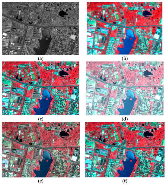
Figure 4.
Visual effects of the four image fusion methods based on GF-1 (R: Band4, G: Band3, B: Band2). (a) shows the panchromatic band gray level image; (b) shows the false-color composite of the original multi-spectral band combination (R: NIR band, G: red band, B green band); (c) shows the false-color composite of the Brovey-fused images; (d) shows the false-color composite of the db2-based wavelet-fused images; (e) shows the false-color composite of the NND-fused images; (f) shows the false-color composite of the GS-fused images.
3.2. Validation
3.2.1. Forest Classification Verification
Table A3, Table A4, Table A5 and Table A6 in Appendix A display the independent validation statistics of the four classification algorithms applied to extract the forest distributions. It was found that the SVM model had an overall classification accuracy of 85.8% and a Kappa coefficient of 0.787 (Table A3, in which the user accuracy of broad-leaved forest, coniferous forest, shrub forest and non-forest reached 90.31%, 76.16%, 49.28% and 91.49%, respectively), the RF model achieved an overall accuracy at 87.8% and a Kappa coefficient of 0.817 (Table A4, in which the user accuracy of broad-leaved forest, coniferous forest, shrub forest and non-forest reached 91.97%, 80.00%, 53.03% and 92.62%, respectively), the Mask-RCNN achieved an overall accuracy of 90.1% and a Kappa coefficient of 0.851 (Table A5, in which the user accuracy of broad-leaved forest, coniferous forest, shrub forest and non-forest reached 93.57%, 85.52%, 63.24% and 92.96%, respectively), and the Swin Transformer coupled with Mask-RCNN had an overall accuracy of 93.9% and a Kappa coefficient of 0.908 (Table A6, in which the user accuracy of broadleaf forest, coniferous forest, shrub forest and non-forest reached 94.94%, 90.13%, 81.13% and 96%, respectively). Obviously, the Swin Transformer coupled with Mask-RCNN outperformed the other three classification models, and its classification results were retained to support subsequent forest distribution change analysis.
3.2.2. Cross-Comparison of the Carbon Density Fitting Results
Figure 5 shows the fitting effects of forest carbon density against forest age by coniferous forest type and broad-leaved forest type, based on the logistic, Richards and Gompertz models. The fitting R2 values of the logistic model, Richards model and Gompertz model for the coniferous forest type were estimated at 0.78, 0.75 and 0.77 respectively, and the fitting R2 values of the three models for the broadleaf forest type were 0.71, 0.70 and 0.71, respectively. Apparently, the logistic model was the best model for simulating carbon density growth in both coniferous forest and broad-leaved forest; thus, it was used to predict the growth of carbon density of each forest stand by specifying the forest type first. Clearly, the fitting performance of the logistic model outperformed the other two models in both coniferous forests and broad-leaved forests, and all the models performed better when fitting coniferous forest data than when fitting broad-leaved forest data in the current study area (Figure 5).
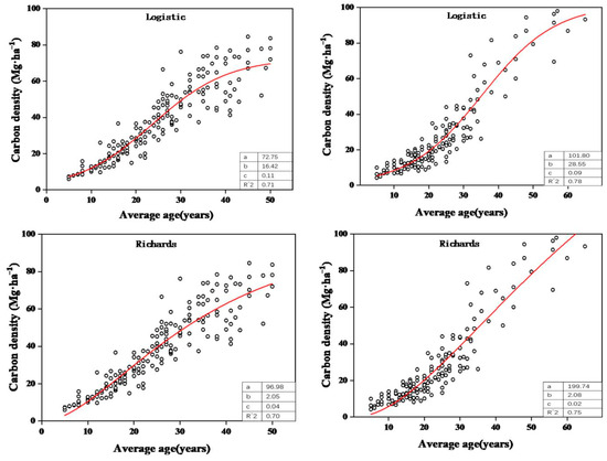
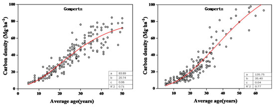
Figure 5.
The fitting relationships between carbon density and forest age for broad-leaved forest (left) and coniferous forest (right) based on the 2017 FMPI data.
Figure 6 shows the cross-validation effects of the fitted models by intercomparing our fitting results with other existing similar studies (Table A7 in Appendix A). In the comparison of coniferous forests, the carbon density results obtained by Justin (Drawing G) [68] were slightly higher than our research results in each age group, and the carbon density results of Li (Drawing C) [69] were also higher than our results in near-mature forest, mature forest and over-mature forest. At the same time, we maintained a high degree of agreement with the carbon density results obtained by Liu (Drawing E) [70], Yan (Drawing F) [71], Wise (Drawing H) [72] and Riahi (Drawing I) [73]. In the comparison of broad-leaved forests, we found that our carbon density results were lower than those of Li (K) [69], Yue (P) [74] and Liu (N) [70] and slightly higher than those of Lan (Drawing L) [75] and Hu (Drawing Q) [76]. But they all reasonably fall within the range of other available findings.
Figure 6.
Comparison of the simulated coniferous forest (left) and broad-leaved forest carbon densities (right) with the results of other similar studies (A is the simulated results in the current analysis).
The cross-validation effect comparison with other existing similar literature shows that the simulated carbon densities of the coniferous forest and the broad-leaved forest at different age groups in the current work were reasonably within the ranges of other existing research results (Figure 6), indicating that the simulated models were reliable and applicable and that they could be used to calculate the carbon densities of persisting forests and newly gained forests in 2020.
3.3. Result Analysis
3.3.1. Forest Classification Extraction Results
Figure 7 displays the forest distribution pattern created from the 2017 FMPI results, Figure 8 shows the 2020 forest type distribution results extracted using the Swin Transformer coupled with the Mask-RCNN model. The forests were principally distributed in the northeastern and southeastern portions of Jiangning District in both 2017 and 2020 (Figure 7 and Figure 8). And there was a total forest area of 41,913.805 hm2 in 2017 and 42,261.315 hm2 in 2020, with a net increase of about 347.51 hm2. Figure 9 conveys the forest change information during the period 2017 to 2020, which was derived from the spatial overlay analysis of the 2017 forest distribution and the 2020 forest distribution. The statistical results of the forest change information map (Figure 9) showed the following: (1) There was a forest gain of 637.164 hm2 during the period 2017 to 2020, and because the newly planted forest lands in 2020 did not take on the spectral signature of the forest type on the GF-1 remote sensing image, the value of 637.164 hm2 might underestimate the actual areas of afforestation that occurred during the period 2017 to 2020. (2) there was a forest loss of 289.654 hm2 during the period 2017 to 2020, and simultaneously, an analysis of forest reduction areas showed that it was mainly due to the construction demand of cities and farmland, and the demand of urban development caused forest reduction. For some regions, forest loss was characterized by small and scattered patches, mainly due to the conversion of forests to farmland. (3) The main reason for the increase in forest in some areas in the past three years was afforestation and greening efforts made by Jiangning District in response to the national policy.
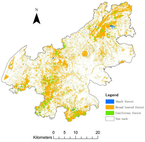
Figure 7.
Forest distribution map of Jiangning in 2017.
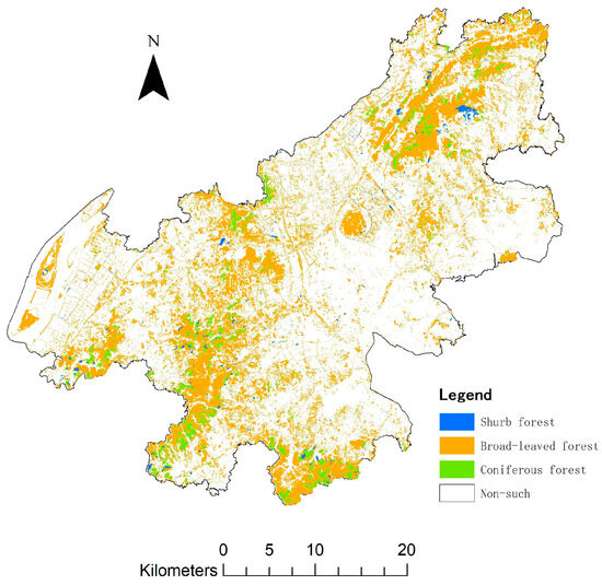
Figure 8.
Forest distribution map of Jiangning in 2020.
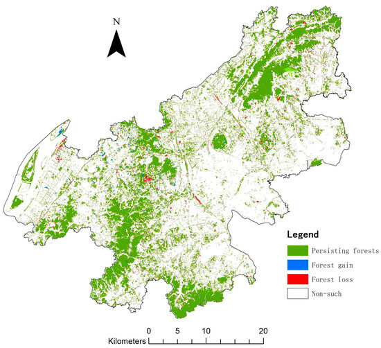
Figure 9.
Forest change map of Jiangning during 2017–2020.
3.3.2. Forest Carbon Storage Measurement and Its Dynamics
Based on the methods mentioned in Section 2.5 and Section 2.6, the forest carbon storage of 2017 was calculated at 125.40 × 10⁴ t, and the shrub forests’ carbon storage was derived at 1.085 × 10⁴ t; thus, the total carbon storage of coniferous forest, broad-leaved forest and shrub forest totaled 126.49 × 10⁴ t in 2017. Based on the distributions of the persisting forests and the newly gained forests, the 2017 FMPI data and the fitted carbon equations, the carbon storage of the persisting forests in 2020 was calculated at 142.53 × 10⁴ t, the carbon storage of forest gains was estimated at 1.04 × 10⁴ t and the carbon storage of the shrub forests in 2020 was estimated at 1.142 × 10⁴ t; thus, the total carbon storage of the forests in 2020 of Jiangning District was estimated at 143.54 × 10⁴ t. Comparing the 2017 total carbon storage with the 2020 carbon storage, we found that there was a net increase in carbon storage of 2.41 × 10⁴ t.
4. Discussion
- (1)
- Forest type extraction effectiveness and reliability
The initial backbone of the improved Mask-RCNN model in this study was replaced by the Swin Transformer model, and the modified framework produced an extraction accuracy that was similar to or even higher than that in other studies that also used this type of approach [28,29]. Cong et al. compared the extraction accuracy of the improved Mask-RCNN model fused with Swin Transformer with the convolutional neural network model embedded with UNet3+ in bell pepper instance detection, and they found that the average detection accuracy, average detection recall, average segmentation accuracy and F1 score were 98.1%, 99.4%, 94.8% and 98.8%, respectively, indicating that the improved Mask-RCNN model fused with Swin Transformer could effectively segment different classes of bell peppers under overexposure, bell pepper overlap and leaf occlusion conditions [77]. Jamali et al. compared multiple models within RF, SVM, VGG-16, 3D CNN, and Swin Transformer to classify coastal wetlands in Saint John, New Brunswick, Canada, and this work demonstrated that Swin Transformer has great potential in classifying complex coastal landscapes [78]. Our results in the current study are consistent with the findings of the above-mentioned two studies and confirm the effectiveness and high accuracy of the proposed framework for forest type extraction applications.
- (2)
- Forest growth model
According to the fitting results of the three forest growth models, logistic, Gompertz and Richards, the logistic model had the best effect. Xu used five growth theory models, namely Compertz, Korf, logistic, Mischerlich and Schumacher, to fit the unit stock of the Masson pine forest and Chinese fir forest in Longquan, Zhejiang, and found that the logistic equation had the best fitting effect, and the coefficient of determination was above 0.85 [79]. Similarly, Rong et al. took Jinguuling Forest Farm in Jilin as a research object and established a stand stock growth model by using five theoretical growth equations: Richards, logistic, single molecule, Gompertz and Korf. Their results showed that the logistic model was the best in Larix artificial forest, mixed broad-leaved forest and mixed coniferous natural forest [80]. The results of the two analyses are consistent with the results of our study, which fully indicates the validity and credibility of the results of this study.
- (3)
- Carbon storage measurement
Based on the 2017 FMPI data, this analysis focused only on the carbon pool of living trees. Forest carbon storage was measured by dominant tree species categories in each forest stand, and the local species-specific parameter values of BEF, carbon content, root-to-stem ratio and basic density of wood compiled from the Second Forestry Carbon Sink Measurement and Monitoring Work Program of Jiangsu Province were used, which made the calculation results more accurate and in line with the forests of Jiangning District of Nanjing City. Further, if the empirical parameters of soil and AGB (above-ground biomass) sample plots surveyed by Fang et al. were taken as a basis, a rough estimation of the soil carbon stock, litter carbon pool and understory shrub and grass carbon pool in the forests of Jiangning District could be performed [42]; thus, our calculation results related to different carbon pools could be expanded to support more a comprehensive assessment of forest carbon fixation capability. However, these parameters are generally regional-scale-oriented, and application of them to the local scale, e.g., Jiangning District, should be locally corrected. Due to the unavailability of field sample data on soil, litter and understory shrub and grass in Jiangning’s forests, the empirical estimations may have some uncertainties and deserve further field sampling validations.
- (4)
- Usage of the measured carbon storage dynamics
The forest change map of Jiangning District (2017–2020) (Figure 7) and the measured forest carbon dynamics provide key references for the development of carbon sink forestry, sustainable forest management and forest protection and utilization measures [81]. The information on forest change and carbon storage will enable administrative agencies to grasp the change magnitude of forest carbon sequestration capacity and future development potential in the whole region, to more accurately and efficiently identify areas suitable for forest growth, and to regularly inventory, update, and release data on carbon-stock-related indicators based on the framework proposed in the current work, helping to continuously explore new paths for forest carbon stock measurement and monitoring [82]. Additionally, the change information will facilitate the adoption of forest quarantine, biological and chemical control, prediction and forecasting, and damage assessment to prevent forest disasters from occurring and to improve forest management effectiveness [83]. Ultimately, this study can provide a technical reference for efficient monitoring of forest status change, and its findings lay an underlying data basis for local agencies to develop targeted forest management policies or measures when pursuing the double-carbon goals (achieving peak CO2 emissions before 2030 and carbon neutrality before 2060).
5. Conclusions
In this study, we developed an efficient framework that integrates deep learning, statistical modeling and GF-1 remote sensing images for the timely evaluation of changes in forest distribution and forest living carbon storage. We particularly fit the local optimal carbon density growth equations by forest type to facilitate the dynamic assessment of standing trees’ carbon storage in Jiangning’s forests between 2017 and 2020. The results showed that Mask-RCNN fused with Swin Transformer had the highest capability in extracting coniferous forest, broad-leaved forest and shrub forest compared to the other three models. Additionally, the net increase in forest area and standing tree carbon storage indicated the effectiveness of the forest management practices implemented by the local agencies. The study findings provide key data and a methodological basis for the development of carbon sink forestry, sustainable forest management and targeted measures for forest conservation and utilization and contribute to pursuing the double-carbon goals (achieving peak CO2 emissions before 2030 and carbon neutrality before 2060 in China).
Author Contributions
Conceptualization, M.L. and D.X.; methodology, J.L. and B.Y.; software, J.L. and B.Y.; validation, J.L. and B.Y.; formal analysis, B.Y.; investigation, J.L. and B.Y.; resources, M.L. and D.X.; data curation, M.L.; writing—original draft preparation, J.L., writing—review and editing, J.L. and M.L.; visualization, J.L., supervision, M.L.; project administration, M.L.; funding acquisition, M.L. and D.X. All authors have read and agreed to the published version of the manuscript.
Funding
This work was jointly funded by the National Natural Science Foundation of China, grant number 31971577, and the Priority Academic Program Development of Jiangsu Higher Education Institutions (PAPD).
Data Availability Statement
The data will be made available by the authors on request.
Conflicts of Interest
Da Xu was employed by Zhejiang Forestry Survey Planning and Design Company Limited. The remaining authors declare that the research was conducted in the absence of any commercial or financial relationships that could be construed as a potential conflict of interest. Zhejiang Forestry Survey Planning and Design Company Limited had no role in the design of the study; in the collection, analyses, or interpretation of data; in the writing of the manuscript, or in the decision to publish the results.
Appendix A

Table A1.
The involved calculation parameters for dominant tree species (groups) in China.
Table A1.
The involved calculation parameters for dominant tree species (groups) in China.
| Number | Dominant Species | BEF | Basic Density of Wood D (t/m³) | Root-to-Stem Ratio | Carbon Content Ratio (tC/t d.m) |
|---|---|---|---|---|---|
| 1 | Red Pine | 1.4251 | 0.4137 | 0.1920 | 0.5141 |
| 2 | Black Pine | 1.8920 | 0.4500 | 0.2180 | 0.5146 |
| 3 | Horsetail Pine | 1.2940 | 0.4482 | 0.1730 | 0.5271 |
| 4 | Overseas Pine | 1.4209 | 0.4894 | 0.2813 | 0.5156 |
| 5 | Wetland Pine | 1.3780 | 0.3590 | 0.2680 | 0.5311 |
| 6 | Torch Pine | 1.5680 | 0.4354 | 0.3380 | 0.5361 |
| 7 | Other Pines | 1.3410 | 0.4649 | 0.1810 | 0.4963 |
| 8 | Fir | 1.2990 | 0.3071 | 0.2030 | 0.5127 |
| 9 | Willow Fir | 1.2710 | 0.2893 | 0.2680 | 0.5331 |
| 10 | Metasequoia | 1.3630 | 0.2740 | 0.3510 | 0.5083 |
| 11 | Pond fir | 1.3580 | 0.3700 | 0.3133 | 0.5156 |
| 12 | Cypress | 1.4580 | 0.4722 | 0.2190 | 0.5088 |
| 13 | Yew (Sequoia) | 1.4477 | 0.3913 | 0.2197 | 0.5156 |
| 14 | Other Fir | 1.3340 | 0.3765 | 0.2420 | 0.5185 |
| 15 | Oak | 1.2880 | 0.6119 | 0.2890 | 0.4798 |
| 16 | Birch | 1.4210 | 0.5270 | 0.2530 | 0.4914 |
| 17 | Water, Hu, Yellow | 1.2930 | 0.4523 | 0.2210 | 0.4620 |
| 18 | Ash | 1.3120 | 0.5462 | 0.3190 | 0.4803 |
| 19 | Walnut | 1.3088 | 0.4302 | 0.2863 | 0.4803 |
| 20 | Camphor | 1.2490 | 0.4649 | 0.2580 | 0.4916 |
| 21 | Nan | 1.2490 | 0.4807 | 0.2580 | 0.5002 |
| 22 | Elm | 1.3683 | 0.4868 | 0.2504 | 0.4803 |
| 23 | Mullein | 1.4090 | 0.5161 | 0.1990 | 0.5115 |
| 24 | Maple | 1.2860 | 0.4860 | 0.3370 | 0.4803 |
| 25 | Other Hardwoods | 1.3850 | 0.6062 | 0.2410 | 0.4901 |
| 26 | Lime | 1.3831 | 0.4177 | 0.1997 | 0.4392 |
| 27 | Sassafras | 1.3130 | 0.4758 | 0.2610 | 0.4848 |
| 28 | Poplar | 1.3940 | 0.3644 | 0.1850 | 0.4502 |
| 29 | Willow | 1.3940 | 0.4409 | 0.1850 | 0.4803 |
| 30 | Paulownia | 1.7870 | 0.2367 | 0.2360 | 0.4695 |
| 31 | Eucalyptus | 1.1930 | 0.5901 | 0.1790 | 0.4748 |
| 32 | Acacia | 1.3860 | 0.5843 | 0.2070 | 0.4666 |
| 33 | Mullein | 1.3440 | 0.6768 | 0.1950 | 0.4893 |
| 34 | Neem | 1.3884 | 0.4389 | 0.1890 | 0.4803 |
| 35 | Other Soft Broadleaf | 1.2730 | 0.4222 | 0.2150 | 0.4502 |
| 36 | Conifer Mix | 1.3646 | 0.3902 | 0.2086 | 0.5168 |
| 37 | Broadleaf Mix | 1.2815 | 0.5222 | 0.2351 | 0.4796 |
| 38 | Needle–Broadleaf Mix | 1.3230 | 0.4754 | 0.2218 | 0.4893 |
Table A2.
Objective evaluation measures of different image fusion algorithms.
Table A2.
Objective evaluation measures of different image fusion algorithms.
| Statistics | Band | Correlation Coefficient | Mean Gradient | Information Entropy | |
|---|---|---|---|---|---|
| Fusion Methods | |||||
| Panchromatic | 18.1610 | 6.2657 | |||
| Multi-spectra | Blue | 10.0761 | 6.5217 | ||
| Green | |||||
| Red | |||||
| NIR | |||||
| GS | Blue | 0.9743 | 63.2020 | 7.6584 | |
| Green | |||||
| Red | |||||
| NIR | |||||
| Brovey | Green | 0.8843 | 14.6312 | 4.6582 | |
| Red | |||||
| NIR | |||||
| Wavelet Transform | Blue | 0.9081 | 1.1443 | 3.8584 | |
| Green | |||||
| Red | |||||
| NIR | |||||
| NNDiffuse | Blue | 0.9094 | 10.0635 | 6.9215 | |
| Green | |||||
| Red | |||||
| NIR | |||||
Table A3.
Accuracy validation statistics of forest type classifications based on SVM.
Table A3.
Accuracy validation statistics of forest type classifications based on SVM.
| Classification Result | |||||||
|---|---|---|---|---|---|---|---|
| Broad-leaved forest | Coniferous forest | Shrub forest | Non-forest | Subtotal | Producer accuracy (%) | ||
| Reference samples | Broad-leaved forest | 354 | 15 | 12 | 13 | 394 | 89.85 |
| Coniferous forest | 17 | 115 | 10 | 11 | 153 | 75.16 | |
| Shrub forest | 10 | 8 | 34 | 9 | 61 | 55.74 | |
| Non-forest | 11 | 13 | 13 | 355 | 392 | 90.56 | |
| Subtotal | 392 | 151 | 69 | 388 | 1000 | ||
| User accuracy (%) | 90.31 | 76.16 | 49.28 | 91.49 | |||
| OA = 85.8% | Kappa = 0.787 | ||||||
Table A4.
Accuracy validation statistics of forest type classifications based on RF.
Table A4.
Accuracy validation statistics of forest type classifications based on RF.
| Classification Result | |||||||
|---|---|---|---|---|---|---|---|
| Broad-leaved forest | Coniferous forest | Shrub forest | Non-forest | Subtotal | Producer accuracy (%) | ||
| Reference samples | Broad-leaved forest | 355 | 13 | 12 | 14 | 394 | 90.10 |
| Coniferous forest | 15 | 124 | 8 | 6 | 153 | 81.05 | |
| Shrub forest | 9 | 8 | 35 | 9 | 61 | 57.38 | |
| Non-forest | 7 | 10 | 11 | 364 | 392 | 92.86 | |
| Subtotal | 386 | 155 | 66 | 393 | 1000 | ||
| User accuracy (%) | 91.97 | 80.00 | 53.03 | 92.62 | |||
| OA = 87.8% | Kappa = 0.817 | ||||||
Table A5.
Accuracy validation statistics of forest type classifications based on Mask-RCNN.
Table A5.
Accuracy validation statistics of forest type classifications based on Mask-RCNN.
| Classification Result | |||||||
|---|---|---|---|---|---|---|---|
| Broad-leaved forest | Coniferous forest | Shrub forest | Non-forest | Subtotal | Producer accuracy (%) | ||
| Reference samples | Broad-leaved forest | 364 | 11 | 9 | 10 | 394 | 92.39 |
| Coniferous forest | 13 | 124 | 7 | 9 | 153 | 81.05 | |
| Shrub forest | 5 | 4 | 43 | 9 | 61 | 70.49 | |
| Non-forest | 7 | 6 | 9 | 370 | 392 | 94.39 | |
| Subtotal | 389 | 145 | 68 | 398 | 1000 | ||
| User accuracy (%) | 93.57 | 85.52 | 63.24 | 92.96 | |||
| OA = 90.1% | Kappa = 0.851 | ||||||
Table A6.
Accuracy validation statistics of forest type classifications based on Mask-RCNN combined with Swin Transformer.
Table A6.
Accuracy validation statistics of forest type classifications based on Mask-RCNN combined with Swin Transformer.
| Classification Result | |||||||
|---|---|---|---|---|---|---|---|
| Broad-leaved forest | Coniferous forest | Shrub forest | Non-forest | Subtotal | Producer accuracy (%) | ||
| Reference samples | Broad-leaved forest | 375 | 8 | 5 | 6 | 394 | 95.18 |
| Coniferous forest | 10 | 137 | 3 | 3 | 153 | 89.54 | |
| Shrub forest | 6 | 5 | 43 | 7 | 61 | 70.49 | |
| Non-forest | 4 | 2 | 2 | 384 | 392 | 97.96 | |
| Subtotal | 395 | 152 | 53 | 400 | 1000 | ||
| User accuracy (%) | 94.94 | 90.13 | 81.13 | 96.00 | |||
| OA = 93.9% | Kappa = 0.908 | ||||||
Table A7.
List of similar studies used to verify the effectiveness and reliability of the simulated carbon density equations.
Table A7.
List of similar studies used to verify the effectiveness and reliability of the simulated carbon density equations.
| Letter | Stand Type | Source | Letter | Stand Type | Source |
|---|---|---|---|---|---|
| B | Coniferous plantation forests | Ali [84] | J | Broad-leaved plantation forests | Li [69] |
| C | Coniferous natural forests | Li [69] | K | Broadleaf natural forests | Li [69] |
| D | Mixed conifer forests | Li [85] | L | Mixed broadleaf forests | Lan [75] |
| E | Mixed coniferous forests | Liu [70] | M | Mixed broadleaf forests | Li [85] |
| F | Coniferous forests | Yan [71] | N | Mixed broadleaf forests | Liu [70] |
| G | Coniferous plantations | Justine [68] | O | Mixed broadleaf forests | Yang [86] |
| H | Coniferous forests | Wise [72] | P | Broadleaf forests | Yue [74] |
| I | Coniferous forests | Riahi [73] | Q | Broad-leaved natural forests | Hu [76] |
References
- Qureshi, A.; Badola, R.; Hussain, S. A review of protocols used for assessment of carbon stock in forested landscapes. Environ. Sci. Policy 2012, 16, 81–89. [Google Scholar] [CrossRef]
- Lal, R.; Smith, P.; Jungkunst, H.F.; Mitsch, W.J.; Lehmann, J. The carbon sequestration potential of terrestrial ecosystems. J. Soil Water Conserv. 2018, 73, 145A–152A. [Google Scholar] [CrossRef]
- Cui, J.; Glatzel, S.; Wang, B. Long-term effects of biochar application on greenhouse gas production and microbial community in temperate forest soils under increasing temperature. Sci. Total Environ. 2021, 767, 145021. [Google Scholar] [CrossRef]
- Zhang, J.; Lin, H.; Li, S. Accurate gas extraction (AGE) under the dual-carbon background: Green low-carbon development pathway and prospect. J. Clean. Prod. 2022, 377, 134372. [Google Scholar] [CrossRef]
- Leite, R.V.; Mohan, M.; Cardil, A. Individual Tree Attribute Estimation and Uniformity Assessment in Fast-Growing Eucalyptus spp. Forest Plantations Using Lidar and Linear Mixed-Effects Models. Remote Sens. 2020, 12, 3599. [Google Scholar] [CrossRef]
- Forrester, D.I.; Benneter, A.; Bouriaud, O. Diversity and competition influence tree allometric relationships developing functions for mixed-species forests. J. Ecol. 2017, 105, 761–774. [Google Scholar] [CrossRef]
- Atkins, J.W.; Costanza, J.; Dahlin, K.M. Scale dependency of lidar-derived forest structural diversity. Methods Ecol. Evol. 2023, 14, 708–723. [Google Scholar] [CrossRef]
- Madonsela, S.; Cho, M.A.; Ramoelo, A.; Mutanga, O. Investigating the relationship between tree species diversity and landsat-8 spectral heterogeneity across multiple phenological stages. Remote Sens. 2021, 13, 2467. [Google Scholar] [CrossRef]
- Huang, C.; Zhang, C.; Liu, Q. Multi-Feature Classification of Optical and SAR Remote Sensing Images for Typical Tropical Plantation Species. Sci. Silvae Sin. 2021, 57, 80–91. (In Chinese) [Google Scholar]
- Nartišs, M.; Melniks, R. Improving pixel-based classification of GRASS GIS with support vector machine. Trans. GIS 2023, 27, 1865–1880. [Google Scholar] [CrossRef]
- Liu, X.; Bo, Y. Object-Based Crop Species Classification Based on the Combination of Airborne Hyperspectral Images and LiDAR Data. Remote Sens. 2015, 7, 922–950. [Google Scholar] [CrossRef]
- Mao, L.; Li, M. Integrating Sentinel Active and Passive Remote Sensing Data to Land Cover Classification in a National Park from GEE Platform. Geomat. Inf. Sci. Wuhan Univ. 2023, 48, 756–764. (In Chinese) [Google Scholar]
- James, G.C.B.; Katerina, P. Using deep convolutional neural networks to forecast spatial patterns of Amazonian deforestation. Methods Ecol. Evol. 2023, 13, 2622–2634. [Google Scholar] [CrossRef]
- Zhao, R.; Yan, R.; Chen, Z. Deep learning and its applications to machine health monitoring. Mech. Syst. Signal Process. 2019, 115, 213–237. [Google Scholar] [CrossRef]
- LeCun, Y.; Bengio, Y.; Hinton, G. Deep learning. Nature 2015, 521, 436–444. [Google Scholar] [CrossRef]
- LeCun, Y.; Boser, B.; Denker, J.S. Backpropagation applied to handwritten zip code recognition. Neural Comput. 1989, 1, 541–551. [Google Scholar] [CrossRef]
- Jeon, E.; Kim, S.; Park, S.; Kwak, J.; Choi, I. Semantic segmentation of seagrass habitat from drone imagery based on deep learning: A comparative study. Ecol. Inform. 2021, 66, 101430. [Google Scholar] [CrossRef]
- He, S.; Du, H.; Zhou, G. Intelligent map of urban forests from high-resolution remotely sensed imagery using object-based u-net-densenet-coupled network. Remote Sens. 2020, 12, 3928. [Google Scholar] [CrossRef]
- Hameed, K.; Chai, D.; Rassau, A. Score-based mask edge improvement of Mask-RCNN for segmentation of fruit and vegetables. Expert Syst. Appl. 2022, 190, 116205. [Google Scholar] [CrossRef]
- Sievänen, R.; Salminen, O.; Lehtonen, A. Carbon stock changes of forest land in Finland under different levels of wood use and climate change. Ann. For. Sci. 2014, 71, 255–265. [Google Scholar] [CrossRef]
- Yuan, L.; Qiu, Z. Mask-RCNN with spatial attention for pedestrian segmentation in cyber–physical systems. Comput. Commun. 2021, 180, 109–114. [Google Scholar] [CrossRef]
- Xie, Y.; Xu, Y.; Hu, C. Urban forestry detection by deep learning method with GaoFen-2 remote sensing images. J. Appl. Remote Sens. 2022, 16, 022206. [Google Scholar] [CrossRef]
- Shi, F.; Yang, B.; Li, M. An improved framework for assessing the impact of different urban development strategies on land cover and ecological quality changes-A case study from Nanjing Jiangbei New Area, China. Ecol. Indic. 2023, 147, 109998. [Google Scholar] [CrossRef]
- Ren, K.; Chen, Z.; Gu, G. Research on infrared small target segmentation algorithm based on improved mask R-CNN. Optik 2023, 272, 170334. [Google Scholar] [CrossRef]
- Carvalho, O.L.F.; de Carvalho Junior, O.A.; Albuquerque, A.O. Instance segmentation for large, multi-channel remote sensing imagery using mask-RCNN and a mosaicking approach. Remote Sens. 2020, 13, 39. [Google Scholar] [CrossRef]
- Vaswani, A.; Shazeer, N.; Parmar, N. Attention is all you need. In Advances in Neural Information Processing Systems; Curran Associates, Inc.: New York, NY, USA, 2017; Volume 30. [Google Scholar]
- Tian, Y.; Bu, X. Lumbar spine image segmentation method based on attention mechanism and Swin Transformer model. Meas. Test. Technol. 2021, 48, 57–61. [Google Scholar]
- Liu, Z.; Lin, Y.; Cao, Y. Swin transformer: Hierarchical vision transformer using shifted windows. In Proceedings of the IEEE/CVF International Conference on Computer Vision, Virtual, 11–17 October 2021; pp. 10012–10022. [Google Scholar] [CrossRef]
- Gao, J.; Zhang, X.; Guo, Y. Research on the optimized pest image instance segmentation method based on the Swin Transformer model. J. Nanjing For. Univ. (Nat. Sci. Ed.) 2023, 47, 1, (Translated from Chinese). [Google Scholar] [CrossRef]
- Gupta, R.; Sharma, L.K. The process-based forest growth model 3-PG for use in forest management: A review. Ecol. Model. 2019, 397, 55–73. [Google Scholar] [CrossRef]
- Pretzsch, H.; Biber, P. Fertilization modifies forest stand growth but not stand density: Consequences for modelling stand dynamics in a changing climate. For. Int. J. For. Res. 2022, 95, 187–200. [Google Scholar] [CrossRef]
- Li, C.; Barclay, H.; Huang, S. Modelling the stand dynamics after a thinning induced partial mortality: A compensatory growth perspective. Front. Plant Sci. 2022, 13, 1044637. [Google Scholar] [CrossRef] [PubMed]
- Satoh, D. Discrete Gompertz equation and model selection between Gompertz and logistic models. Int. J. Forecast. 2021, 37, 1192–1211. [Google Scholar] [CrossRef]
- Zhao, J.; Hu, H.; Wang, J. Forest Carbon Reserve Calculation and Comprehensive Economic Value Evaluation: A Forest Management Model Based on Both Biomass Expansion Factor Method and Total Forest Value. Int. J. Environ. Res. Public Health 2022, 19, 15925. [Google Scholar] [CrossRef] [PubMed]
- Clément, J.B.; Sous, D.; Bouchette, F. A Richards’ equation-based model for wave-resolving simulation of variably-saturated beach groundwater flow dynamics. J. Hydrol. 2023, 619, 129344. [Google Scholar] [CrossRef]
- Jiang, X.; Wen, S.; Yu, X. Studies on the Variable—Density Whole Stand Model of Cunninghamia lanceolata Plantations and Its Application. J. Fujian For. Sci. Technol. 2000, 27, 22–25, (Translated from Chinese). [Google Scholar]
- Feng, Z.; Xiong, N.; Wang, J.; Li, X. Establishment and Study of Full Stand Models for Sidebar Artificial Forests in Beijing City. J. Beijing For. Univ. 2008, S1, 214–227, (Translated from Chinese). [Google Scholar]
- Wang, M.; Wei, X.; Wei, Y.; Wang, M. Population structure and dynamic characteristics of rare and endangered plant Ormosia hosiei in Sichuan and Guizhou Province. Chin. Guihaia 2023, 45, 179, (Translated from Chinese). [Google Scholar]
- Luo, M.; Wang, Y.; Xie, Y. Combination of feature selection and catboost for prediction: The first application to the estimation of aboveground biomass. Forests 2021, 12, 216. [Google Scholar] [CrossRef]
- Zhang, B.; Liu, G.; Feng, Z. Constructing a Model of Poplus spp. Growth Rate Based on the Model Fusion and Analysis of Its Growth Rate Differences and Distribution Characteristics under Different Classes of Environmental Indicators. Forests 2023, 14, 2073. [Google Scholar] [CrossRef]
- Piao, S.; Fang, J.; Ciais, P. The carbon balance of terrestrial ecosystems in China. Nature 2009, 458, 1009–1013. [Google Scholar] [CrossRef]
- Fang, J.; Wang, G.; Liu, G. Forest biomass of China: An estimate based on the biomass-volume relationship. Ecol. Appl. 1998, 8, 1084. [Google Scholar]
- Wulder, M.; White, J.; Nelson, R. Lidar sampling for large-area forest characterization: A review. Remote Sens. Environ. 2012, 121, 196–209. [Google Scholar] [CrossRef]
- Vincent, W.; Gao, J. Towards refined estimation of vegetation carbon stock in Auckland, New Zealand using WorldView-2 and LiDAR data: The impact of scaling. Int. J. Remote Sens. 2019, 40, 8727–8747. [Google Scholar]
- Nelson, R.; Hyde, P. Investigating RaDAR–LiDAR synergy in a North Carolina pine forest. Remote Sens. Environ. 2007, 110, 98–108. [Google Scholar] [CrossRef]
- Vatandaşlar, C.; Abdikan, S. Carbon stock estimation by dual-polarized synthetic aperture radar (SAR) and forest inventory data in a Mediterranean forest landscape. J. For. Res. 2022, 33, 827–838. [Google Scholar] [CrossRef]
- Wang, S.; Kobayashi, K.; Takanashi, S. Estimating divergent forest carbon stocks and sinks via a knife set approach. J. Environ. Manag. 2023, 330, 117114. [Google Scholar] [CrossRef] [PubMed]
- Cao, X.; Ke, C.; Ran, J. Research on urban land use expansion based on GIS technology—A case study of Jiangning District, Nanjing. Resour. Sci. 2008, 30, 385–391, (Translated from Chinese). [Google Scholar]
- Gillespie, A.R.; Kahle, A.B.; Walker, R.E. Color enhancement of highly correlated images-Channel Ratio and ‘Chromaticity’ Transformation Techniques. Remote Sens. Environ. 1987, 22, 343–365. [Google Scholar] [CrossRef]
- Hamid, R.S. Improved Adaptive Brovey as a New Method for Image Fusion. arXiv 2018, arXiv:1807.09610. [Google Scholar]
- Ehlers, M.; Klonus, S.; Johan, A. Multi-sensor image fusion for pansharpening in remote sensing. Int. J. Image Data Fusion 2010, 1, 25–45. [Google Scholar] [CrossRef]
- Witharana, C.; Larue, M.A.; Lynch, H.J. Benchmarking of data fusion algorithms in support of earth observation based Antarctic wildlife monitoring. J. Photogramm. Remote Sens. 2016, 113, 124–143. [Google Scholar] [CrossRef]
- Chen, Y.; Sun, K. Quality evaluation of Gaofen-2 image fusion method. Surv. Mapp. Sci. 2017, 42, 35–40. [Google Scholar]
- Vijayaraj, V.; Younan, N.H.; O’Hara, C.G. Quantitative analysis of pansharpened images. Opt. Eng. 2006, 45, 828. [Google Scholar] [CrossRef]
- Ducay, R.; Messinger, D.W. Image fusion of hyperspectral and multispectral imagery using nearest-neighbor diffusion. J. Appl. Remote Sens. 2023, 17, 024504. [Google Scholar] [CrossRef]
- Oliveira, R.J.; Caldeira, B.; Teixidó, T. Geophysical data fusion of ground-penetrating radar and magnetic datasets using 2D wavelet transform and singular value decomposition. Front. Earth Sci. 2022, 10, 1011999. [Google Scholar] [CrossRef]
- Yuan, Y.; Zhang, J.; Chang, B. Objective quality evaluation of visible and infrared color fusion image. Opt. Eng. 2011, 50, 033202. [Google Scholar] [CrossRef]
- Guo, M.; Li, B.; Shao, Z. Objective image fusion evaluation method for target recognition based on target quality factor. Multimed. Syst. 2022, 28, 495–510. [Google Scholar] [CrossRef]
- Sarkar, J.; Rashid, M. Visualizing mean, median, mean deviation, and standard deviation of a set of numbers. Am. Stat. 2016, 70, 304–312. [Google Scholar] [CrossRef]
- Edjabou, M.E.; Martín-Fernández, J.A.; Scheutz, C. Statistical analysis of solid waste composition data: Arithmetic mean, standard deviation and correlation coefficients. Waste Manag. 2017, 69, 13–23. [Google Scholar] [CrossRef]
- Zhu, H.; Jia, G.; Zhang, Q. Detecting Offshore Drilling Rigs with Multitemporal NDWI: A Case Study in the Caspian Sea. Remote Sens. 2021, 13, 1576. [Google Scholar] [CrossRef]
- Liao, L.; Song, J.; Wang, J. Bayesian method for building frequent Landsat-like NDVI datasets by integrating MODIS and Landsat NDVI. Remote Sens. 2016, 8, 452. [Google Scholar] [CrossRef]
- Roy, D.P.; Li, J.; Zhang, H.K. Examination of Sentinel-2A multi-spectral instrument (MSI) reflectance anisotropy and the suitability of a general method to normalize MSI reflectance to nadir BRDF adjusted reflectance. Remote Sens. Environ. 2017, 199, 25–38. [Google Scholar] [CrossRef]
- Zheng, G.; Li, X.; Zhou, L.; Yang, J.; Ren, L. Development of a gray-level co-occurrence matrix-based texture orientation estimation method and its application in sea surface wind direction retrieval from SAR imagery. IEEE Trans. Geosci. Remote Sens. 2018, 56, 5244–5260. [Google Scholar] [CrossRef]
- Wang, F.; Bhattacharya, A.; Gelfand, A.E. Process modeling for slope and aspect with application to elevation data maps. Test 2018, 27, 749–772. [Google Scholar] [CrossRef]
- Ring, M.; Eskofier, B.M. An approximation of the Gaussian RBF kernel for efficient classification with SVMs. Pattern Recognit. Lett. 2016, 84, 107–113. [Google Scholar] [CrossRef]
- Nonini, L.; Fiala, M. Estimation of carbon storage of forest biomass for voluntary carbon markets: Preliminary results. J. For. Res. 2021, 32, 329–338. [Google Scholar] [CrossRef]
- Justin, M.F. Dynamics of biomass and carbon sequestration across a chronosequence of masson pine plantations. J. Geophys. Res. Biogeosciences 2017, 122, 578–591. [Google Scholar] [CrossRef]
- Li, Q. Carbon Stock and Carbon Sequestration Potential of Arboreal Forests in China from 2010 to 2050; China Academy of Forestry Sciences: Beijing, China, 2016; (Translated from Chinese). [Google Scholar]
- Liu, W. Carbon stock and allocation characteristics of public welfare forests in Baisanzuo National Park. J. Ecol. 2021, 40, 1–10, (Translated from Chinese). [Google Scholar]
- Yan, R. Dynamic analysis and potential prediction of carbon stock in arboreal forests in Chongqing. For. Econ. 2019, 41, 70–77, (Translated from Chinese). [Google Scholar]
- Wise, M. Implications of limiting CO2 concentrations for land use and energy. Science 2009, 324, 1183–1186. [Google Scholar] [CrossRef]
- Riahi, K. Scenarios of long-term socio-economic and environmental development under climate stabilization. Technol. Forecast. Soc. Change 2007, 74, 887–935. [Google Scholar] [CrossRef]
- Yue, J. Carbon Sequestration Dynamics, Potential and Impact mechanisms of Major Forest Types in Gansu; University of Chinese Academy of Sciences (Research Centre for Soil and Water Conservation and Ecological Environment, Ministry of Education, Chinese Academy of Sciences): Yangling, China, 2018; (Translated from Chinese). [Google Scholar]
- Lan, T.; Gu, J.; Wen, Z. Spatial distribution characteristics of carbon storage density in typical mixed fir and broadleaf forests. Energy Rep. 2021, 7, 7315–7322. [Google Scholar] [CrossRef]
- Hu, W.; Wang, X. Comparison of ecosystem carbon density between sharp-toothed Quercus serrata and cork oak forests. J. For. Environ. 2017, 37, 8–15, (Translated from Chinese). [Google Scholar]
- Cong, P.; Li, S.; Zhou, J. Research on instance segmentation algorithm of greenhouse sweet pepper detection based on improved mask RCNN. Agronomy 2023, 13, 196. [Google Scholar] [CrossRef]
- Jamali, A.; Mahdianpari, M. Swin transformer and deep convolutional neural networks for coastal wetland classification using sentinel-1, sentinel-2, and LiDAR data. Remote Sens. 2022, 14, 359. [Google Scholar] [CrossRef]
- Xu, Q. Construction and Simulation of Stand Growth Model; Zhejiang Agricultural Forest University: Hangzhou, China, 2015. [Google Scholar]
- Rong, J.; Liu, D. Growth model of stand stock of main forest types in overcut forest area of northeast China. Appl. Res. 2011, 25, 30–34. [Google Scholar] [CrossRef]
- Kaya, A.; Bettinger, P.; Boston, K.; Akbulut, R.; Ucar, Z. Optimisation in forest management. Curr. For. Rep. 2016, 2, 1–17. [Google Scholar] [CrossRef]
- Paul, T.; Kimberley, M.O.; Beets, P.N. Natural forests in New Zealand–a large terrestrial carbon pool in a national state of equilibrium. For. Ecosyst. 2021, 8, 34. [Google Scholar] [CrossRef]
- Runting, R.K.; Ruslandi; Griscom, B.W. Larger gains from improved management over sparing–sharing for tropical forests. Nat. Sustain. 2019, 2, 53–61. [Google Scholar] [CrossRef]
- Ali, A.; Ahmad, A.; Akhtar, K. Patterns of biomass, carbon, and soil properties in masson pine (Pinus massoniana Lamb) plantations with different stand ages and management practices. Forests 2019, 10, 645. [Google Scholar] [CrossRef]
- Li, Y. Carbon stocks in forest ecosystems and their distribution characteristics in Zhejiang Province. J. Plant Ecol. 2016, 40, 354–363, (Translated from Chinese). [Google Scholar]
- Yang, J.; He, Y.; Caspersen, J.P. Delineating individual tree crowns in an uneven-aged, mixed broadleaf forest using multispectral watershed segmentation and multiscale fitting. IEEE J. Sel. Top. Appl. Earth Obs. Remote Sens. 2016, 10, 1390–1401. [Google Scholar] [CrossRef]
Disclaimer/Publisher’s Note: The statements, opinions and data contained in all publications are solely those of the individual author(s) and contributor(s) and not of MDPI and/or the editor(s). MDPI and/or the editor(s) disclaim responsibility for any injury to people or property resulting from any ideas, methods, instructions or products referred to in the content. |
© 2024 by the authors. Licensee MDPI, Basel, Switzerland. This article is an open access article distributed under the terms and conditions of the Creative Commons Attribution (CC BY) license (https://creativecommons.org/licenses/by/4.0/).