Abstract
Urban forest parks offer valuable spaces for walking activities that benefit both physical and mental health. However, trails in current park designs are often underutilised, and the scene layout does not fully meet the preferences of walkers. Therefore, understanding the connection between scene characteristics and walking preferences is essential. This study aimed to develop an ensemble protocol to assess the role of scene characteristics in walking preferences, using Shanghai Gongqing Forest Park as an illustrative example. A walking preference heat map was created using a combination of crowdsourced GPS data. The scene characteristics were quantified using panoramic photographs, drone orthophotos, computer vision, and deep learning techniques. Taking spatial dependence into account, the key findings include the following: (1) From an overhead view, the shortest paths, waterbody density, and recreational facility selection positively influenced walking preferences, while secondary asphalt trails had a negative effect. (2) At the eye level, aesthetically pleasing landscape elements, such as flowers and bridges, attracted more pedestrians, while closed trails were less favoured. (3) Eye-level features explained 43.5% of the variation in walking preference, with a stronger influence on walking preference compared to 22.4% for overhead features. (4) Natural elements were generally more significant than artificial ones; the feature ranking of significant impact was flowers > NACHr1000 > visual perception > water body density > bridge > SVF > retail > entertainment > asphalt. This study proposes a flexible protocol that provides urban forest park managers and planners with practical tools to create a more walker-friendly environment and more accurate trail alignment, as well as a solid empirical basis for assessing the use of urban forest parks.
1. Introduction
Urban forests serve as vital spaces for residents to engage in physical activity, with walking being the most popular form of exercise in these settings [1,2]. Compared with urban walking, walking through a forest environment not only enhances physical health but also boosts cognitive functions and fosters positive emotions [3,4]. A study from Taiwan showed that walking in a forest setting is more beneficial to cardiovascular function than walking in the city [4]. Research by Lin et al., Lim et al., and Rose et al. also indicates that visits to urban forests can help alleviate depression and anxiety, restore attentional focus, and improve mental well-being [5,6,7].
Urban forest parks are essential components of these green spaces and offer residents a daily retreat [8]. For instance, suburban forest parks in Shanghai attract millions of visitors annually, and in Japan, families with children and young adults frequently enjoy walking together in urban forest parks [2,9,10]. People are drawn to perform activities in well-designed walking environments; previous studies have highlighted the macroscopic environmental characteristics of urban forest parks as key to influencing visitation and have examined the attributes that encourage walking [11,12]. However, few studies have addressed the relationship between fine-scale scene characteristics and walking preferences. Therefore, on one hand, to foster a more walkable environment and ensure that the needs of walkers are met, it is essential to quantify the impact of these scene characteristics on walking preferences in urban forest parks.
On the other hand, exploring the relationship between specific scene characteristics of trails and walking preferences can help optimise trail alignment in urban forest parks. Trail alignment refers to the process of designing and planning a park to reasonably determine the direction and layout of its trails. This not only affects the traffic flow and organisation within the park but also directly impacts the overall visitor experience and the visual quality of the landscape. However, forest parks are large in area, and in large parks, the traditional empirically driven trail alignment method may not match people’s actual route selection preferences, which may lead to low utilisation of trails after planning. For example, a study in the Danube National Park in Austria showed that 50% of the tourists used only 20% of the total path length [13]. In Gongqing Forest Park in Shanghai, China, visitors walked on an average of 21 out of 105 trails [2]. Visitors to most forest parks tend to concentrate their activities in fewer spaces, thus reducing the utilisation of other spaces. For example, Smailes and Smith found that 16% of 105 locations counted contained 50% of the total number of visitors throughout the year [14].
Thus, it is necessary to understand the relationship between fine-scaled scene characteristics and walking preferences in urban forest parks in order to guide the future planning and management. To fill this gap, we summarise the shortcomings of the current research: First, detailed protocols for assessing the role of urban forest park scene characteristics in people’s walking preferences are lacking. Existing protocols have focused on the role of trail characteristics at the macro level. Most of these studies have focused on the characteristics of a single trail or its surrounding environment and have revealed the factors that affect trail preferences [2,3]. For instance, Zhai et al. provided a protocol based on spatial syntax theory and field tracking using GPS devices [2]. Conceptualising trail attributes in two dimensions, including trail metric and configurational attributes, the results showed that walking preference in urban forest parks is related to the properties of the trails as a unit. Some protocols invite visitors to rate the expected trail scenes. They usually explore each user’s landscape preferences by creating landscape selection sets and discrete models [9,15,16,17]. However, because landscape datasets are usually set according to the expectations of researchers, they can only provide one alternative to the walking environment and a vague understanding of the general characteristics of the trail area; quantifying the actual characteristics of the user’s surroundings in different locations is difficult. In general, these protocols ignore the scene characteristics of individual user locations on a finer scale. Consequently, some of the scene layouts and element designs in the actual planning of a forest park may not meet people’s walking needs.
Second, the system for evaluating the characteristics of forest park scenes must be improved. Mainstream studies have explained the influence of park environmental characteristics from a top-view perspective [1,11,18]. In terms of top-view attributes, social, natural, and facility functional attributes are often mentioned, in addition to the often-mentioned effects of the trails themselves. This includes factors such as visitor numbers, recreational facilities, vegetation cover, and proportion of water bodies, all thought to promote or inhibit walking enthusiasm [1,19]. Eye-level views can provide a direct perception for visitors to experience environmental exposure [20]; however, the question of how and to what extent environmental characteristics within the line of sight affect visitors’ walking preferences has not received sufficient attention. Sporadic subjective and objective features at eye level have been shown to influence visitors’ walking preferences in forest parks, such as the presence of dead wood, interpretive signs and leisure seats, scene cleanliness, safety, and line-of-sight permeability [3,21,22,23]. However, none of these studies have focused on whether the proportion of scene elements in the frame within the visual range affects the walking preferences in urban forest parks. Furthermore, the relative importance of eye-level and overhead views has not been confirmed.
Third, large-scale sample sizes and dynamic data sources to quantify actual walking preferences in urban forest parks are lacking. Questionnaires, structured interviews, and follow-up monitoring are the main methods used for walking preference studies in forest parks, with the disadvantage that data recording is time-consuming and has a low throughput [2,24,25]. For example, there is sampling bias in randomly accessing a population, and the data are usually cross-sectional, which may lead to errors in inferring the impact of the relationship [2]. Low response rates are also common in survey research, and these problems make it difficult for survey results to reflect actual usage [26].
In the context of a new data environment, the emergence of GPS crowdsourcing tracking provides a new data source for walking activities [27,28,29] that can record the behavioural patterns of walkers in a fine-scale position at the user’s individual level. Moreover, on-site observations and UAVs are widely used to record a site’s objective features and explore people’s preferences for green spaces [26,30,31]. Recent research has also used a combination of panoramic photographs and deep learning techniques to semantically segment panoramic photographs obtained from on-site observations to quantify the characteristics of objective scene elements [32]. These methods provide new opportunities for studying the relationship between scene characteristics and walking preferences.
In this context, we selected Shanghai Gongqing Forest Park as the research site, obtained multisource data based on the tools and methods mentioned above, and quantified the relationship between scene characteristics and walking preferences. This study made the following contributions. First, we proposed a fine-scale and controllable protocol using multiple techniques and methods to assess the role of the scene characteristics of urban forest parks in people’s walking preferences. This protocol helps optimise the trail alignment and spatial design of forest parks. Second, we improved the system for evaluating the characteristics of forest park scenes in two dimensions: a top-view and an eye-level dimension, with particular attention paid to the eye-level characteristics. Third, we explored the relative importance of these two dimensions in influencing walking preferences. Fourth, we used the spatial autoregression model to explore the spatial dependence effect and then used explainable machine learning values to discover the important scene factors affecting walking preferences and the ways they affect them.
In summary, the reason for conducting this study is that understanding the impact of scene characteristics on walking preferences helps create a walkable urban forest park environment and optimise trail alignment within the park. Our purpose was to assess the influence of urban forest park scenario characteristics on walking preferences by developing a new protocol. Through this protocol, we would like to understand some of the forest park scenario factors that affect walking preferences and how they are affected in order to provide some references for planning and management. Consequently, we asked the following questions and conducted this study from June to August, 2024. The questions are as follows: (1) To what extent can the developed new assessment protocol explain the effects of scenario features on walking preferences? (2) How and what are the factors influencing walking preference from the top-view perspective? (3) How and what are the factors influencing walking preference from the eye-level perspective? (4) What is the relative contribution of scene characteristics from the top-view and eye-level perspectives on walking preferences?
2. Materials and Methods
2.1. Study Area
This study chose Shanghai Gongqing Forest Park as the research site, which is located in the northeastern part of the Yangpu District, Shanghai, west of the Huangpu River, as shown in Figure 1b. Gongqing Forest Park has a large number of annual visitors and a high daily visitor intensity. According to statistics, the park receives approximately two million visitors annually, with a maximum daily capacity of 130,000 visitors https://lhsr.sh.gov.cn/gyhd/20210623/e7da767b-26d2-4cf9-b043-e3dc6356ded3.html (accessed on 9 November 2024).
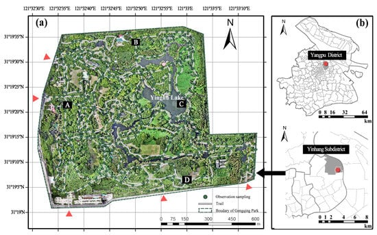
Figure 1.
The extent of Gongqing Forest Park, Shanghai, China: (a) the orthographic projection; (b) the site location in Shanghai.
The park is divided into two parts, north and south, of which the North Park is mainly a forest landscape, while the South Park is intersected by an urban expressway and has a very different style. Therefore, in this study, we chose only the North Park as the research site. The North Park covers an area of 1631 acres, with clear main and secondary roads suitable for walking tours, and includes a variety of recreational and leisure programmes, such as a forest train and racecourse, boating on Yinghu Lake, and bird watching on the promenade. Figure 1a is an orthographic projection of Gonqing Forest Park taken from a UAV, with points A, B, C, D indicating the locations of the aforementioned programmes, respectively.
2.2. Study Protocol
This study proposes a protocol (Figure 2) to assess the influence of urban forest park scene characteristics on walking preferences. The protocol was used in this study. It involved the following six steps: First, the location of the scene preferred by walkers was investigated using an open crowdsourced GPS application, and a walking heat map was generated using kernel density estimation (KDE). Second, observational samples were collected as research units using on-site observation methods. Based on previous research, a scene-characteristic system was constructed from two perspectives, top view and eye level, and included seven attributes (top view: trail metric, trail configuration, and natural, social, and facility function; eye level: objective features and subjective perception). Panoramic photos, unmanned aerial vehicles (UAVs), network big data, computer vision (CV), and deep learning (DL) techniques were then used for quantification. Third, correlation tests were used to determine the scene features that were significantly related to walking preference. Fourth, the ordinary least squares (OLS) model was used to compare the relative contributions of the top-view and eye-level dimensions to explain walking preferences in urban forest parks. Fifth, a SAC model was used to explain the spatial dependence effect of the scene feature system in the joint action of the top view and eye level. Features with insignificant effects after considering spatial autocorrelation were excluded. Finally, we used SHAP values to rank the importance of significant features and showed the SHAP dependencies in a box plot to explain the influence modes of significant features.
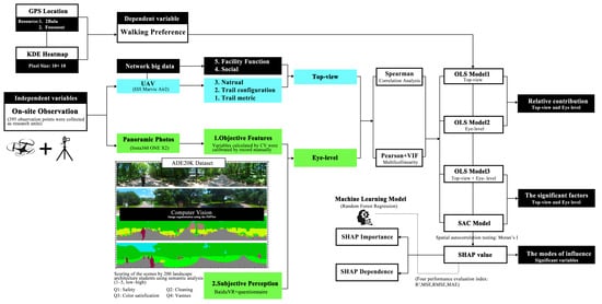
Figure 2.
The protocol of assessing the influence of scene characteristics on walking preference in urban forest parks.
2.3. People’s Preference for Walking
2.3.1. Acquisition of a Walker’s GPS Location from Crowed-Sourced Data
GPS is one of the most commonly used data sources for tracking activities like walking and is widely used to determine walking preferences [2,33]. In this study, GPS location data were used as the dependent variable obtained from the crowdsourcing applications 2Bulu and Foooooot [28,34]. Using web crawler technology, we extracted the timestamp, username, Keyhole Markup Language (KML), GPS Exchange Format (GPX) tracks, and track point data from a Uniform Resource Locator (URL) list. In this study, we used the Selenium package in Python to identify and capture web elements containing the target information and to address slider problems. Notably, because the website cannot directly match the timestamp with the latitude and longitude information of the track points, the KML and GPX tracks must be converted to the CSV format, the times must be matched, and the latitude and longitude information of the track points must be extracted again from the tracks corresponding to similar times. The GPX and KML data were parsed using the xml package. The smallest timestamp unit was the second. Because the data are public, the entire collection process does not involve ethical privacy issues. Considering the problem of scene changes due to long-term temporal changes, we only extracted GPS location information from the past eight years. In addition, we only recorded the locations of walking activities, since our research was focused on walkers.
2.3.2. Screening for a Walker’s GPS Location
The GPS track points were uploaded by the walkers themselves; therefore, there was noise. To reflect the walkers’ preference for the scene more clearly, these track points needed to be screened using one guideline: if the same user repeatedly uploaded two or more fixes at the same location at the same time, these GPS track points were merged into one, and the duplicates were deleted. Figure 3a,b show the spatial distribution of all GPS locations crawled by 2Bulu and Foooooot.
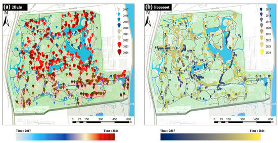
Figure 3.
GPS locations from crowdsourced data. GPS locations of all walkers in the Gongqing Forest Park from the (a) 2Bulu and (b) Foooooot applications. Gross data from 2017 to 2024 were collected.
2.3.3. Generating Walking Preferences
To display the spatial distribution patterns of walking preferences, we used KDE in ArcGIS to smooth the track points representing walking preferences. When processing geospatial information, the KDE generates a density surface by rendering each cell based on the kernel density at the pixel centre. For each observed geographic point, KDE fits a kernel function assuming that each point is continuously distributed within its kernel window [35]. In this study, the kernel estimator with the kernel function K was defined as follows [36]:
where h is the window width, also called the smoothing parameter or bandwidth.
2.4. On-Site Observation Method
In this study, we collected 395 scene points as the basic units of scene characteristics using on-site observations. The scene-characteristic data were acquired using a panoramic camera and a UAV. The panoramic camera was an Insta360 ONE X2 (Shenzhen Arashi Vision Co., Ltd., Shenzhen, China) and the UAV was a DJI Mavic Air 2 (DJ-Innovations, Shenzhen, China). On-site observations were divided into five steps, as shown below:
- All the data were collected in a non-rainy environment. The image acquisition tasks in this study were conducted from June 10 to 15 and from July 3 to 10, 2024, for a total of 14 days. The experiment was conducted daily from 8:00 to 18:00.
- The starting point for UAV shooting was conducted at a low altitude (flight altitude of 100 metres above the ground) with a gimbal inclination of −90°. An aerial survey was conducted on 4 July 2024 with sufficient sunshine at the site and no electromagnetic interference. Both vertical and horizontal shots were spaced 30 m apart to ensure that the overlap between the horizontal and vertical pixels in each image was greater than 1/3 to obtain a digital orthophoto of the park using Pix4Dmapper (version 4.4.12) software [26].
- The panoramic camera was placed at 90° to the ground at a height of 160 cm on the centreline of the road and shot every 20–80 m, taking one image at a time. During this period, the photographer needed to hide himself and ensure that no scenes had closely interfering objects blocking the lens. Figure 4 shows the on-site observation process using a panoramic camera.
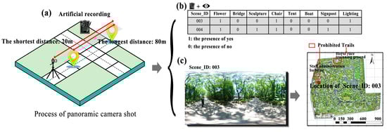 Figure 4. Illustration of the process of on-site observation with the panorama camera and the positioning of photos: (a) the illustration of a panoramic camera by on-site observation; (b) the form of dichotomous scene-characteristic variables that need to be recorded manually; (c) an illustration of the position of panoramic photos.
 - The collection locations for the panoramic camera were trails that were freely accessible to walkers. Some of the unopened spaces and trails prohibited to visitors were not captured, such as the staff administration building in the west and the horse race training ground in the north.
- The dichotomous scene-characteristic variables at eye level were recorded manually to calibrate the data calculated using CV, and the panoramic camera shooting points were mapped onto the orthophoto of the UAV.
2.5. Variables of Scene Characteristics
The scene characteristics are the independent variables in this study. We assessed the scene characteristics of the Gongqing Forest Park in two dimensions: top view and eye level. The top-view dimension was found to have a significant effect on walking. Therefore, most variables were obtained from previous studies. The eye-level dimension was added as an innovation. Table 1 presents the sources, data descriptions, and processing methods for the variables. Details of all these are explained next.
2.5.1. Top-View Dimension
Five attributes were summarised in the top-view dimension: trail metrics, trail configuration, social facility, functional facility, and natural attributes.
Nine variables were selected to describe the trail attributes (four from the metrics attribute and five from the configuration attribute). We mapped the trail network of Gongqing Forest Park based on the orthographic projections from the UAV. The trail network in this study was based on the approach of Zhai et al. for trail segmentation [2], in which the trail between two intersections is considered as one trail without any other intersections in between. Trails that are connected, such as the three short, interconnected trails, act as loop intersections. Detailed descriptions and sources of the data are recorded in Table 1. Stone pavement, gravel, asphalt, and natural materials were chosen for the trail surface because they are commonly used materials in forest trail studies. Trail configuration variables were spatial syntactic variables that measured the spatial properties of the network.
Social and functional facility attributes were obtained through the API interfaces of the Baidu heat map and Amap, a Chinese map service provider. Functional facilities play an important role in walking preferences in forest scenes [4]. In addition to the frequently mentioned recreational amenities, we added three other types of amenities: retail, landscape, and cultural. Shannon diversity was used to represent the diversity of amenities and was calculated based on the four facility types using the following formula:
where represents the proportion of the functional facility to the total number of individuals.
Variables in the natural attribute were trained using DL on orthophoto projections to recognise the canopy and water bodies. The canopy and waterbody samples were manually divided into two categories (category 1: canopy/waterbody, category 2: others), and pixel-wise supervised training was used; the classifier was chosen to be SVM with a maximum number of 500 samples per class, all of which were implemented in ArcGIS pro3.1.
2.5.2. Eye-Level Dimension
All variables for eye-level environmental dimensions were based on on-site observations. The variables for the objective features were selected from the ADE20k dataset, which describes the outdoor scenes. We selected 15 features that best described the forest scene and segmented the panoramic images using the CV and DL techniques. However, some features are more suitable for dichotomous variables. The effect of the signpost on the walker was due to the presence of the signpost in the field of view rather than its area. In addition, subjective perception variables require access to a wider range of perceptions. Specifically, eye-level variables must be treated in four ways:
- The first six scene elements in Table 1 are continuous variables separated from the ADE20k dataset; the PSPNet algorithm was used to segment the image from the panoramic camera and calculate the pixel values [32,37]. No evident wall elements were present in the park; therefore, walls and buildings were combined as architectural elements. However, panoramic images are not suitable for the direct extraction of elements because of image distortion in the upper and lower parts of the panoramic images [38,39]. Tsai and Chang reported that panoramic images have less distortion in the centre [39]. Therefore, they suggested locating the visual elements in the central part with a spacing of ±30 cm based on the vertical field of view of the camera lens. This method was used in this study, as shown in Figure 5.
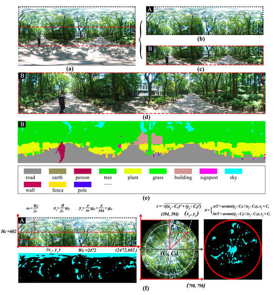 Figure 5. Semantic segmentation based on PSPNet. (a,c,d) The area within the red dashed line is where we extract the eye-level scene characteristics; (a,b) the area within the black dashed line is where we calculate the SVF value; (e) the semantic segmentation result; (f) the fisheye conversion process and the result of calculating the SVF.
 - The sky view factor (SVF) is a continuous variable calculated based on semantically segmented sky elements and is used to measure the objective enclosure of the environment [38]. Fisheye (hemispherical) images were generated using the method developed by Xia et al. [40] to quantify the SVF values in the upper half of the panoramic image based on the section shown in Figure 5b. Next, the SVF values were calculated using Equation (2). Figure 5f shows a schematic representation of the fisheye process.
- 3.
- Eight variables were dichotomous. They included flowers, bridges, sculptures, chairs, tents, signposts, road lights, and boats. All variables were first segmented using CV and then manually recorded by on-site observations to verify the accuracy. A value of 0 indicates absence and a value of 1 indicates presence.
- 4.
- Subjective perception variables of the scenes were quantified using the Semantic Differential (SD) method. The SD method is a relatively commonly used psychometric method whose distinctive feature is the quantification of psychologically rated feelings [41]. In this study, 395 panoramic photos were uploaded to the Baidu Virtual Reality platform, and the average subjective ratings from 200 landscape architecture students for each scene were collected using a questionnaire star platform. During the experiment, participants were asked to browse each VR scene and then assess the subjective perception of the five indicators according to the criteria described in Table 1, which were divided into five levels, with corresponding scores of 1, 2, 3, 4, and 5 (score 1 indicates the worst level, and score 5 indicates the best level) [32]. Figure 6a shows a sample scene scoring for one of the subjects, and Figure 6b shows a few examples of high and low scores for each question.
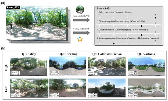 Figure 6. Schematic overview of subjective perception variables: (a) one sample of scoring for objective perception (scene encoding: 003); (b) a few examples of high and low scores.

Table 1.
The descriptive statistics of independent variables.
Table 1.
The descriptive statistics of independent variables.
| Variables | Data Description and Extraction | Data Source | Reference |
|---|---|---|---|
| Top-View Dimension | |||
| Trail Metric | |||
| Trail surface | Observe the surface material of each trail on-site, including four types: stone pavement, gravel, asphalt, and natural). | Manual recording on-site of each observation point | Arnberger et al. [15] Wimpey and Marion [16] |
| Width | Measure by on-site observation. | Zhang et al. [42] | |
| Length | Extract the length of each trail segment from the road network. | Road network from orthophoto map of UAV | Zhai et al. [2] |
| Distance to gate | Calculate the distance from each observation point to the nearest entrance. | Park entrance and location of observation points | Orellana et al. [43] Zhai et al. [2] |
| Trail Configuration | |||
| Connectivity | Calculate based on space syntax theory using DepthMap software 0.8.0. To compare systems of different sizes, normalised angular integration/choice (NAIN/NACH) with two radii (200 and 1000 m) was taken in this study according to the range of the park scales to represent walking accessibility. | Manually draw road network from orthophoto map of UAV | Zhai et al. [2] Wang et al. [26] |
| Integration—NAINr200m | |||
| Integration—NAINr1000m | |||
| Choice—NACHIr200m | |||
| Choice—NACHr1000m | |||
| Social | |||
| Visitor count | Extract the raster value of each observation point from the Baidu heat map. | Baidu heat map API | Zhang et al. [44] |
| Natural | |||
| Canopy density | Visual interpretation of canopy/waterbody layers and training of UAV orthophotos using pixel-oriented supervised classification to generate a high-resolution canopy/waterbody cover map (category 1: canopy, category 2: other), calculating the proportion of the area of the canopy/waterbody in the 20 m/50 m/80 m buffer generated at each observation point. | Orthophoto map of UAV | Agimass et al. [1] |
| Waterbody density | Gerstenberg et al. [11] Bjerke et al. [45] Kang et al. [46] | ||
| Functional Facility | |||
| Shannon diversity | Calculate Shannon–Wiener index. | Amap | Jiang et al. [38] |
| Facility type | POI type of recreation, retail, landscape, and cultural facilities. | Wang et al. [3] | |
| Eye-Level Dimension | |||
| Objective Feature | |||
| Architecture | PSPNet semantic segmentation framework using Python script; the dataset is ADE20K, and the architecture represents the gross of walls and building elements. | 395 panoramic photos | Qiu et al. [47] Dong et al. [48] |
| Tree | |||
| Grass | |||
| Plant | |||
| Earth | |||
| Fence | |||
| SVF | Generate fisheye and calculate SVF values using Python script. | 395 panoramic photos | Li et al. [49] Xia et al. [40] |
| Flower | Categorical: 1 = element was presented in picture. 0 = element was not presented in picture. Each presence was calibrated by the PSPNet semantic segmentation framework, then further calibrated by on-site observation; the flower category represents the garden, flowerbeds, and continuous flower belts that appear in the scene. | Panoramic photos of 395 on-site observation points and calibration accuracy through on-site manual recording | Qiu et al. [47] Dong et al. [48] Yang et al. [30] |
| Bridge | |||
| Boat | |||
| Sculpture | |||
| Chair | |||
| Tent | |||
| Signpost | |||
| Road light | |||
| Subjective Perception | |||
| Safety | A total of 200 students with a background in landscape architecture were invited to view the VR photos and rate each scene using the SD method (five levels: 1, 2, 3, 4, 5), using these scales: Safety perception: insecure ~ secure Cleaning perception: dirty and messy ~ clean and tidy. Colour satisfaction: colour incongruity ~ colour harmony. Vastness perception: low sense of vastness ~ high sense of vastness. | Panoramic photos from 395 on-site observation points and VR scoring | Heyman et al. [50] Henderson et al. [23] Reichhart and Arnberger et al. [19] |
| Cleaning | |||
| Colour satisfaction | |||
| Vastness |
2.6. Correlation Analysis and OLS Analysis
The Spearman or Pearson coefficient is typically used to explore the degree of bivariate correlation, and OLS is an ordinary linear model widely used to examine the key role of independent variables on dependent variables [22]. We first performed a correlation analysis between scene characteristics and walking preferences to identify associated variables and eliminate unrelated variables in two steps:
- Correlation analysis between scene characteristics and walking preferences, according to the histogram of dependent variables, was conducted using the Spearman or Pearson correlation coefficient.
- Diagnosing multicollinearity was diagnosed by eliminating variables with a variance inflation factor (VIF) >5 and using Pearson analysis to ensure the stability of the coefficient of statistical modelling.
We then created three OLS models to compare the contributions of the top-view and eye-level dimensions:
OLS Model 1: walking preference (y)~top-view dimension.
OLS Model 2: walking preference (y)~eye-level dimension.
OLS Model 3: walking preference (y)~ top-view dimension + eye-level dimension.
Prior to this, the problem of modifiable area units was considered, which results in bias in the aggregation of geographic data in the statistical results [48]. The top-view dimensions were built within 20, 50, and 80 m buffers to verify the stability of the model. Buffers with better results were then used for OLS and spatial modelling analyses.
2.7. Spatial Effect and Modelling Statistics
Previous studies have shown that park usage and activities can be influenced by the spatial distribution of interior park attributes, leading to spatial autocorrelation [51]. Consequently, a spatial autocorrelation test was required for the scene-characteristic walking preference dataset. The spatial autocorrelation effect was assessed using the Moran’s I test. A significant correlation of Moran’s I values indicates that the OLS model is spatially autocorrelated. In such cases, we must build a corresponding spatial model for further analysis based on the correlations of robust Lagrange multipliers (lags) and robust Lagrange multipliers (errors) in OLS to ensure the accuracy of the regression results. In this study, we need to consider the SAC model with a spatially lagged dependent variable and a spatially autocorrelated error term. Its calculation method is as follows [47]:
where is the KDE value of walking preference in sampling point i; is the KDE value of walking preference in point ; is the spatial autocorrelation coefficient; is the spatial weight matrix; is the coefficient of the variables we chose; is the value of the variables in point ; is a vector of the spatial autoregressive error term; is the coefficient of the spatial dependence in error terms; and is the error term.
2.8. Relative Importance and Single-Factor Influence by SHAP
SHAP is a popular method for interpretable machine learning. It calculates the Shapley values based on game theory, where each Shapley value represents the extent to which a variable in a single sample contributes to a predicted dependent variable [52]. The Shapley value allows us to calculate the relative importance of scene feature variables in influencing walking preferences and in how individual factors are influenced [53]. When the Shapley value was greater than zero, a positive influence was found on the dependent variable, and when it was less than zero, a negative influence was observed.
In this study, the significant scene variables identified in the SAC model were ranked using a summary plot of SHAP values. Due to the relatively small sample employed in this study, box plots were used to visualise each variable in stages, and the trends of the box plots were used to determine the influencing role of a single factor. The SHAP value needs to be interpreted based on a trained machine learning model. This study adopted a random forest model, which is more popular in urban research, as a modified tree-modelling algorithm [54]. In the training process, we split the training and test sets in a ratio of 7:3 and measured the performance of the random forest using four metrics: R2, MSE, RMSE, and MAE.
3. Results
3.1. Descriptive Statistics for Walking Preference
Figure 7a presents a heat map of the KDE-generated walking preferences. Figure 7b shows the spatial distribution of the KDE raster values for the 395 sampling points collected through on-site observation. The raster values varied between 0 and 0.012, with a pixel size of 10 × 10, showing a right-skewed distribution. The spatial distribution of walking preferences showed that hotspot areas were mainly dispersed along the centre of the trail network on both sides, showing evident spatial heterogeneity.
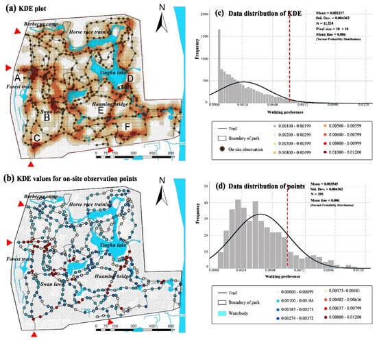
Figure 7.
KDE heat map and the value of walking preference for each on-site observation point: (a) KDE plot for walking preference; (b) the raster value extracted from the KDE plot of each on-site observation point; (c,d) the walking preference data distribution trends of the KDE and points, respectively.
An evident phenomenon is that the distribution of heat is higher along the water’s edge, for example, in the Water Forest, Yinghu Scenic Area, and some trails around the Huaming Bridge, which correspond to positions A, D, and E in Figure 7a, respectively. In addition, several recreational spaces also serve as areas of concentration for walks or stopovers, such as the swan lawn and children’s playground at position B and the entrance plaza at position C, with retail and shade facilities. Position F is a promenade used for bird watching. The heat level was lower in large woodland areas and some lanes. To further explore the correlations and factors influencing walking preference, the following analyses were conducted.
3.2. Correlation and Multicollinearity
Table 2 presents the relative importance of the three buffer zone groups, with adjusted R2 values of 0.224, 0.212, and 0.192. All the F-statistics were significant, confirming the validity of the models. Because the OLS model with the 20-metre buffer demonstrated the highest goodness of fit, we focused on this buffer group for further analysis, specifically within the top-view dimension. To ensure that the model coefficients aligned with the expected linear trend, we assessed the multicollinearity for all variables within the buffer range, excluding those with a VIF greater than five.
Table 2.
The relative importance of buffer zones among three scales (Models 1).
The data on walking preferences exhibited a right-skewed distribution. Therefore, Spearman’s correlation analysis was used to assess the significance of the correlations with scene preferences [55]. As shown in Figure 8, Spearman’s analysis identified variables from both the top-view and eye-level groups that were significantly correlated (p < 0.05) with the walking preference. A total of 24 variables showed significant correlations, with 21 positively correlated and 3 negatively correlated. In the top-view group, the significant variables included three trail materials (stone pavement, asphalt, and natural surfaces), trail width, connectivity, NAINr200m, NAINr1000m, NACHIr200m, NACHr1000m, water body density (natural attributes), Shannon diversity index, and recreational and retail facilities (functional facility attributes). For the eye-level group, the key variables included earth, fences, flowers, SVF, bridges, and sculptures, as well as four subjective perception variables under objective characteristics.
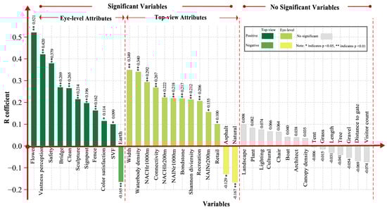
Figure 8.
Significant variables of scene characteristics correlated with walking preference and the ranking importance of the significant variables.
Figure 8 presents the rank order of the correlations between the top-view and eye-level variable groups and walking preferences. Overall, the variables in the eye-level group showed stronger correlations with walking preference than those in the top-view group. To diagnose multicollinearity issues among the 24 significant variables retained, we followed a two-step exclusion process. Initially, variables with a VIF greater than five were removed [56]. However, some model coefficients still displayed directions inconsistent with the expected linear trends. To address this, a second exclusion was performed based on Pearson’s correlation coefficients. After extensive testing, we found that when the correlation between variables fell within the range of −0.3 to 0.3, the direction of the OLS coefficients could be corrected.
The Pearson exclusion criteria were guided by the strength of the correlations between the significant scenario features and the dependent variable, with the independent variables showing higher correlations being retained. For instance, the Pearson coefficients for “flowers and connectivity” and “flowers and sculpture” exceeded 0.3, but the correlation between flowers and the dependent variable was 0.521. By contrast, the correlations for connectivity and sculpture were only 0.267 and 0.214, respectively, leading to their exclusion.
Moreover, although both the soil and fence passed the VIF and Pearson tests, the directions of their coefficients remained inconsistent with the linear trend and were subsequently eliminated. Figure 9 illustrates the results of the Pearson analysis, showing that variables such as stone pavement, connectivity, and NAIN, along with 12 other variables, were excluded. Ultimately, 12 stable explanatory variables were retained in the final OLS model interpretation. The statistical results of these variables are presented in Table 3.
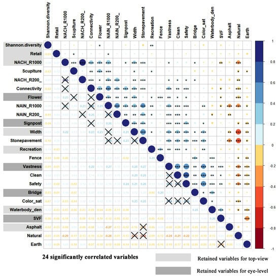
Figure 9.
Pearson correlations among the 24 significant variables, where grey parts are the retained variables that can be used for the OLS analysis. Notes: * p < 0.1; ** p < 0.05; *** p < 0.001.
Table 3.
Statistical results of variables after multicollinearity diagnosis.
3.3. OLS Analysis and the Relative Importance of Variable Group
Table 4 and Table 5 present the results of the relative importance of the top-view dimension (Model 1) and eye-level dimension (Model 2) analysed using the OLS model. The F-statistics for both Models 1 and 2 were significant, with adjusted R2 values of 0.224 and 0.435, respectively, indicating that the variables in the eye-level dimension have higher explanatory power for people’s walking preferences when comparing the two dimensions.
Table 4.
The OLS results of the top-view dimension.
Table 5.
The OLS results of the eye-level dimension.
OLS Model 3 combined these two sets of dimensions. Compared to the separate group of eye-level dimensions, the adjusted R2 of the merged OLS model was not very high (from 0.435 to 0.503), implying that the variables in the top-view dimension did not provide practical improvements and that the variables in the eye-level dimension were the key factors influencing people’s walking preference.
3.4. Moran’s I Test and Spatial Model Results
We performed Moran’s I test (999 permutations) on the residuals in Model 3, and the spatial weight matrix W was “rook”. The Moran I value of the OLS residuals was 0.219 with a p-value = 0.001 < 0.05 (Figure 10, left). This indicates that the OLS residuals had a significant positive spatial autocorrelation. In addition, both the robust Lagrange multiplier (lag) and robust Lagrange multiplier (error) were significant (Table 6), indicating that both spatial lag and error effects were present. Therefore, the SAC model was chosen to eliminate both the lagged dependent variable and spatially lagged error term in the spatial process to account for spatial interactions. The Moran’s I value of the residuals of the SAC model was −0.028 (p = 0.226 > 0.05 (Figure 10, right)), implying that the spatial autocorrelation was not significant and was well handled by the SAC model. In addition, the Moran’s I value of the residuals of the SAC model was significantly lower than that of the OLS Model 4. The R2 value was substantially higher, from 0.513 to 0.685 (SAC model); therefore, we interpreted the results based on SAC.
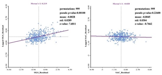
Figure 10.
The left figure shows the residual Moran’s I for OLS; the right shows the residual Moran’s I for SAC.
Table 6.
The OLS and SAC results of all dimensions.
The SAC results showed that the 12 explanatory stable variables included 9 significant variables, 5 from the top-view group and 4 from the eye-level group, namely, water body density, asphalt, NACHr1000, recreation, retail, flower, bridge, SVF, and vastness perception. In addition, Wy, as a spatially lagged variable, also had a significant effect, suggesting that spatial dependence must be considered when understanding walking preferences. Therefore, the Wy variable was added to the random forest model; the results are explained based on the SAC model.
3.5. Feature Importance and Single-Factor Influence
The testing performance of the random forest model is shown in Figure 11a; R2 is 0.675, which means that these nine key features explained 67.5% of the effect. The MSE, RMSE, and MAE were 0.011, 0.104, and 0.080, respectively, indicating that the deviation of the model-predicted value from the true value was very small on average, that no extreme error to increase the overall error was observed, and that the overall fit was reliable.
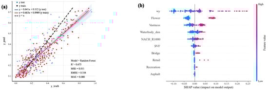
Figure 11.
Model performance of random forest, and the ranking importance of significant variables: (a) the fitting of the training and test sets in the random forest and the status of the performance evaluation metrics; (b) the summary plot of SHAP, showing the ranking of gross variables.
The SHAP values calculate the importance ranking and influence mode of the features, which contain the results of some threshold effects in addition to linear relationships [57]. The results for the feature importance are shown in Figure 11b. The influence of spatially lagged variables was the most important, followed by flowers, vastness perception, NACHr1000, waterbody density, SVF, bridges, retail facilities, recreational facilities, and asphalt. In summary, apart from spatially lagged variables, the top-ranked factors were primarily natural elements, while man-made elements also had an influence but were ranked lower.
We show the SHAP dependency results for each scene factor in stages using box plots, where continuous variables are split into octiles and dichotomous variables are divided into two stages. SHAP dependency analysis demonstrated that the majority of scene factors varied in a linear pattern (Figure 12). For continuous variables, perceived vastness had a positive effect on walking preference after exceeding 3.52 points. Although there are still some scenarios with negative contributions, more than a quarter of the scenes had already increased walking enthusiasm owing to the spaciousness of the environment. When the NACHr1000 value reached 0.55, three-quarters of the scenarios increased walking preferences, and after reaching 0.58, all the scenarios contributed positively. This indicated that a trail network with a high degree of connectivity enhances the willingness of a person to walk.
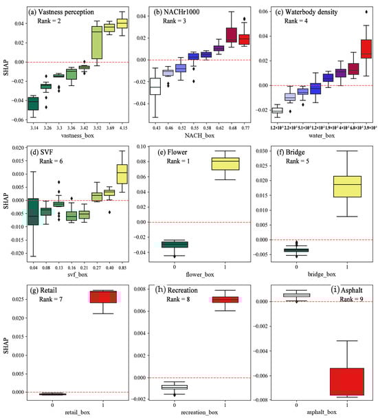
Figure 12.
The SHAP dependence of each key factor is displayed in box plots.
The effect of water body density on walking preference remained positive after reaching 0.04, and walking activity increased as the variable value increased. This clearly showed that the aquatic environment was an attractive area for walking. Regarding the SVF, most scenarios contributed positively to walking heat after the SVF value reached 0.19. Additionally, a small proportion of the SVF values at 0.03 and 0.09 also had a positive contribution, although the proportion was low. SVF values of approximately 0.06, 0.11, and 0.14 made a negative contribution, indicating that in most spaces, lower SVF values were less conducive to encouraging walking.
Among the dichotomous variables, asphalt paths had a negative impact on walking, indicating that asphalt paths in Gongqing Forest Park were not conducive to walking activities. In contrast, retail and entertainment facilities positively affected walking, as walking heat maps were more active around large entertainment venues and convenience stores. Furthermore, in the eye-level dimension, the flower and bridge elements also had a positive influence.
4. Discussion
4.1. A Protocol for Assessing the Role of Scene Characteristics in Walking Preference
Urban forest parks provide natural outdoor spaces for physical exercise and social interaction, which are beneficial for mental and physical health [3,4]. Well-designed park trails can encourage visitors to engage in walking activities [23]. However, improving the utilisation rate of forest park trails remains a significant planning and design challenge [2]. This study proposes a controllable protocol for assessing the influence of urban forest park features on walking preferences. The protocol aimed to clarify the park features preferred by walkers, providing a basis for enhancing the accuracy of trail alignment and the quality of scene design in forest parks.
Compared with traditional methods that rely on surveillance equipment or on-site tracking [25,33], this protocol used crowdsourced data and KDE analysis to quickly generate spatial distribution heat maps of walking preferences. This data collection method was convenient, and it effectively captured walkers’ spatial preferences within forest parks. Additionally, through a systematic review of the existing literature, and considering the scale and perspective of walking units, this study further established a comprehensive variable system that synthesised seven common attributes of green spaces from both the “top-view” and “eye-level” perspectives. Taking Gongqing Forest Park as an example, and accounting for spatial autocorrelation, the results showed that the features from these two perspectives could explain 68.5% of the variation in walking preferences, validating the strong explanatory power and practical utility of this variable system for assessing walking behaviours in urban forest parks.
Unlike conventional methods that use scenic image sets and surveys to collect park feature data [9,15,16,17], this protocol employed panoramic images captured from specific points on-site and orthophotos captured by drones. It combined CV and DL technologies and utilised VR platforms and SD analysis to quantify park features. This new method not only objectively quantified the physical characteristics of park environments but also captured subjective perceptions, providing a more comprehensive perspective for studying the impact of park features on walking behaviours.
The integrated attributes and features of trails have been comprehensively studied in relation to walking behaviour in forest parks [9,33]. To promote more refined measurements of walking spaces, this study further narrowed the analytical units to specific locations of individual users. This study concluded that specific environmental features at individual locations in a forest park are important factors in stimulating walking activities. This protocol offers insights for future research, allowing researchers to systematically analyse the features that influence walkers in a single urban forest park, the mechanisms of their influence, and their relative importance. This can provide targeted guidance for park managers and planners, optimise trail alignment, and improve park utilisation and visitor experience.
4.2. Significance of Scene Characteristics in Affecting Walking Preference
This study provides a comprehensive assessment of the different aspects of forest park scenes and reveals nine key factors that are significantly correlated with walking preferences. These factors included one attribute of trail configuration from the top view (NACHr1000), one attribute of nature (water body density), two attributes of functional facilities (retail and recreational facilities), one attribute of trail metrics (asphalt), one subjective perception attribute (vastness perception), and three objective characteristic attributes (SVF, flower, and bridge).
4.2.1. The Significance of the Top-View Attribute in Influencing Walking Preferences
Trail configuration attributes significantly affect trail utilisation rates. Many studies have shown that spatial topological properties such as control and integration play key roles in pathway network planning [2,58], which was also validated by our correlation analysis. More importantly, we found that choice—that is, the frequency of using the shortest path in the pathway network—had a particularly strong impact on walking behaviour. Additionally, setting short paths in the overall network was more effective in encouraging walking than setting local short paths (NACHr1000 > NACHr200). In the case of Gongqing Forest Park, short-distance trails often connected multiple key activity nodes, providing greater flexibility for walkers, thereby becoming walking hotspots. If the goal is to improve trail utilisation, designing straight roads that lead to active nodes may offer the most stable value.
The positive impact of water bodies in urban forests on walking behaviour has been confirmed multiple times. The results of this study align with previous findings [12], with the highest walking intensity observed in areas with water-based activities such as wetland forests and the Yinghu Scenic Area. Hamstead et al. and Zhang et al. pointed out that visitor activities along waterbodies may be related to the attractiveness of water-based recreational facilities [22,59]. Increasing water-based recreational activities not only enhances the entertainment value of the park but also increases the intensity of walking activities in the surrounding areas.
In terms of functional attributes, our study validates the commonly held view that setting entertainment facilities in forest environments helps stimulate interest in walking [3,22]. Additionally, the presence of retail facilities was positively correlated with walking preferences, especially in areas near shops, restaurants, and other consumer venues where walking activities are more frequent. Recent tourism-oriented planning experiences support these findings. For example, Wang et al. used crowdsourced data (e.g., from Dianping) and map data to extract POIs and assess tourist preferences in rural forest scenes [26] and found that consumer-support factors had a greater influence on walking behaviour than non-consumer-support factors. Entertainment and retail facilities can enhance the tourist value of parks. We advocate that planners understand the recreational needs of tourists in the park to improve the content and layout of internal facilities in a targeted manner, with the ultimate goal of increasing the attractiveness of the walking space.
Theoretically, asphalt pavements may facilitate walking convenience [60], but we found that asphalt pavements inhibit walking passion. The discrepancy with the previous literature may be due to trail classification, as our correlation results suggest that both natural and gravel surfaces similarly deter walking, whereas stone pavement has the opposite effect. This may be because the asphalt, natural, and gravel surfaces in Gongqing Forest Park are primarily used for secondary trails or small paths, whereas the main trails are made of stone pavement. All the results indicate that the classification of trails may be more important than the material in influencing walking preferences. However, owing to the limitations of this single case study, future research will require more case studies and systematic research to explore the differences between trail classification and material preferences and to balance their relative importance.
4.2.2. The Significance of Eye-Level Attributes in Influencing Walking Preferences
In terms of objective features, landscaping elements with aesthetic value are considered important factors in attracting visitors [30,61,62]. Our study indicated that the walking areas surrounding flower beds and gardens exhibited a higher intensity. Landscape bridges were identified as the major factors stimulating walking. Bridges not only serve as aesthetically pleasing design elements but also act as important transportation links to waterfront areas, where walkers are more likely to engage in activities. SVF, often used to measure the closure of a space, was found to have an overall positive effect on forest walking preferences. However, its positive impact becomes significant only when the SVF exceeds 0.2, which may be related to the vegetation coverage threshold [22].
Vastness perception, a subjective perception attribute, is positively correlated with walking preference. Heyman et al. and Bjerke et al. also noted that visual transparency is a factor affecting visitors’ use of forest environments, with semi-open forests providing better visibility than dense forests [45,50]. Therefore, we recommend that park managers regularly maintain trails and pay attention to the density of surrounding facilities and plants.
4.2.3. The Contributions of Top-View and Eye-Level Factors on Walking
In this case study, we found that both top-view and eye-level features had a significant statistical impact on walking preferences in urban forest parks. In the comparative analysis, eye-level features demonstrated a higher relative importance, explaining 43.5% of the variation in walking preferences.
Based on the feature importance and threshold effect, we found that natural elements had a slightly greater impact on walking than did artificial elements (the feature ranking of significant impact was flowers > NACHr1000 > visual perception > water body density > bridge > SVF > retail > entertainment > asphalt), whereas artificial elements may have had a negative impact on walking in some cases. This issue is still debated among academics. Baumeister et al. found artificial infrastructure to be the most important factor when using physical landscape features to explain recreational value hotspots in urban forests [63]. In contrast, Gerstenberge et al. found that an artificial environment reduces the intensity of pedestrian use, and that natural features are more important [11]. These studies compared various urban forest options at the city scale, whereas our study focused on the characteristics of the scene within a single park and provided a deeper understanding of small-scale environments.
4.3. Theoratical Implication
From a technical perspective, this study builds upon traditional field survey experiences while fully utilising interdisciplinary technologies to develop a novel protocol for hierarchical data processing. This protocol integrates GPS crowdsourced data, panoramic images, drone imagery, and computer vision techniques, employing regression and interpretable models to reflect the influence of urban forest park scene characteristics on walking preferences. Thus, the technological integration in this research addresses issues prevalent in traditional methods, such as insufficient sample sizes for walking activities, low survey response rates, and the inability to quantify the image proportions of scene elements. Moreover, this integrated approach proposes a paradigm that is compatible with the analysis of other physical activity subjects and can be further optimised for different research objectives. Beyond walking, it is also applicable to activities like running, cycling, and jogging.
From a scope perspective, this study expands the understanding of walking preferences in urban forests from macro-level trail characteristics to more detailed scene features. Building upon the summary of trail characteristics, it provides a more systematic assessment framework for scene features. By examining and refining the conclusions derived from macro-level trail characteristics from both top-view and eye-level perspectives, this study finds that this assessment framework based on urban forest park scene characteristics can explain 68.5% of the variance in walking preferences.
4.4. Limitations and Future Studies
This study had several limitations. First, the results of the feature influence were based on a specific case of the generalised protocol proposed in this study. Thus, there are some limitations to the selection of influencing factors. For example, in urban forest parks dominated by mountainous landscapes, certain features such as water bodies or bridges may not be present. However, the protocol proposed in this study to assess the relationship between park features and walking preferences is universal and adaptable. Future studies should adopt this protocol and select appropriate indicators based on the specific characteristics of the park to achieve more accurate results. Second, although the validity and usability of the two crowdsourced geospatial big data platforms, 2Bulu and Foot, have been verified [28,64,65], these data sources do not provide demographic details such as age, gender, education level, or other sociodemographic characteristics from the GPS data. This limitation is particularly relevant for older adults, whose behaviours may be underrepresented. Future studies should incorporate field surveys to explore actual walking behaviour patterns in forest parks. Third, although the ADE20k dataset is widely used to describe outdoor scenes, including forest and urban park environments [26,66], its feature selection is still primarily oriented toward typical urban characteristics. In other words, specific features of urban forest parks, such as deadwood and ground cover types, could not be quantified using this dataset. Future research should aim to develop more representative datasets for forest environments, possibly leveraging advanced DL algorithms to enhance the precision of feature extraction. Fourth, further investigation is required to understand the mechanisms through which park features influence walking preferences. The goal of this study was not to establish a causal relationship between walking preferences and park features but to explore this relationship through correlation analysis, particularly by incorporating objective eye-level features—the value of top-view and eye-level dimensions—in walking preference research. Given the complexity of the factors influencing walking intensity, there could be reverse causality or mediating effects of perception, walking motivation, or individual characteristics [67]. Other nonenvironmental factors that have the potential to correlate with walking preferences, such as ticket prices and ecological value [22], should also be considered in future studies to better understand their underlying mechanisms. Finally, perception is multisensory in nature. This study was mainly based on the visual level; however, other senses, such as hearing and smell, may also influence the choice of walking route, which deserves further investigation in future studies.
5. Conclusions
This study developed an ensemble protocol that combines multiple techniques to assess how urban forest park scene characteristics influence walking preferences, aiming to optimise trail alignment accuracy and scene design quality. Unlike previous methods, this protocol examines user-level preferences by analysing walkers’ individual locations using crowdsourced GPS data and KDE for preference mapping. It refines scene assessment into two main dimensions: top view and eye level. Observations collected through on-site sampling were quantified with panoramic cameras, drones, computer vision, and deep learning. Key scene characteristics influencing walking behaviour were identified and ranked using OLS models, spatial autoregression, and SHAP values. Using Shanghai’s Gongqing Forest Park as a case study, results showed visitors prefer short, convenient paths and favour natural landscapes over built environments, underscoring the importance of ecological preservation. However, integrating man-made elements, like entertainment and retail facilities, can enhance visitor experience. Trail openness and visual permeability were also significant, suggesting the importance of attention to facility layout, vegetation density, and regular trail maintenance. This adaptive protocol allows park planners to flexibly adjust landscape choices based on the park’s unique scene characteristics. Future research should focus on expanding the forest scene dataset, exploring other influencing factors, and studying the driving mechanisms of changes in walking behaviour. Even other sensory factors such as hearing and smell can be considered when following this protocol. This research provides valuable insights for improving the usability of urban forest parks.
Author Contributions
Conceptualisation, J.Z. and H.J.; methodology, J.Z. and H.J.; software, J.Z.; validation, J.Z., H.J., W.Y. and B.Q.; formal analysis, J.Z.; investigation, J.Z., H.J. and W.Y.; resources, J.Z.; data curation, J.Z; writing—original draft preparation, J.Z.; writing—review and editing, J.Z.; visualisation, J.Z.; supervision, B.Q.; project administration, B.Q.; funding acquisition, B.Q. All authors have read and agreed to the published version of the manuscript.
Funding
This research was funded by the National Natural Science Foundation of China (NSFC) General Project (Grant No. 31971721).
Data Availability Statement
The data presented in this study are available upon request from the author. Images employed for the study will be available online for readers.
Conflicts of Interest
The authors declare no conflicts of interest.
References
- Agimass, F.; Lundhede, T.; Panduro, T.E.; Jacobsen, J.B. The Choice of Forest Site for Recreation: A Revealed Preference Analysis Using Spatial Data. Ecosyst. Serv. 2018, 31, 445–454. [Google Scholar] [CrossRef]
- Zhai, Y.; Korça Baran, P.; Wu, C. Can Trail Spatial Attributes Predict Trail Use Level in Urban Forest Park? An Examination Integrating GPS Data and Space Syntax Theory. Urban For. Urban Green. 2018, 29, 171–182. [Google Scholar] [CrossRef]
- Wang, X.; Zhang, J.; Wu, C. Users’ Recreation Choices and Setting Preferences for Trails in Urban Forests in Nanjing, China. Urban For. Urban Green. 2022, 73, 127602. [Google Scholar] [CrossRef]
- Tsao, T.-M.; Hwang, J.-S.; Lin, S.-T.; Wu, C.; Tsai, M.-J.; Su, T.-C. Forest Bathing Is Better than Walking in Urban Park: Comparison of Cardiac and Vascular Function between Urban and Forest Parks. Int. J. Environ. Res. Public Health 2022, 19, 3451. [Google Scholar] [CrossRef] [PubMed]
- Lin, W.; Zeng, C.; Bao, Z.; Jin, H. The Therapeutic Look up: Stress Reduction and Attention Restoration Vary According to the Sky-Leaf-Trunk (SLT) Ratio in Canopy Landscapes. Landsc. Urban Plan. 2023, 234, 104730. [Google Scholar] [CrossRef]
- Lim, Y.; Kim, J.; Khil, T.; Yi, J.; Kim, D. Effects of the Forest Healing Program on Depression, Cognition, and the Autonomic Nervous System in the Elderly with Cognitive Decline. J. People Plants Environ. 2021, 24, 107–117. [Google Scholar] [CrossRef]
- Rosa, C.D.; Larson, L.R.; Collado, S.; Profice, C.C. Forest Therapy Can Prevent and Treat Depression: Evidence from Meta-Analyses. Urban For. Urban Green. 2021, 57, 126943. [Google Scholar] [CrossRef]
- Zhai, Y.; Baran, P.K.; Wu, C. Spatial Distributions and Use Patterns of User Groups in Urban Forest Parks: An Examination Utilizing GPS Tracker. Urban For. Urban Green. 2018, 35, 32–44. [Google Scholar] [CrossRef]
- Arnberger, A.; Aikoh, T.; Eder, R.; Shoji, Y.; Mieno, T. How Many People Should Be in the Urban Forest? A Comparison of Trail Preferences of Vienna and Sapporo Forest Visitor Segments. Urban For. Urban Green. 2010, 9, 215–225. [Google Scholar] [CrossRef]
- Oku, H.; Fukamachi, K. The Differences in Scenic Perception of Forest Visitors through Their Attributes and Recreational Activity. Landsc. Urban Plan. 2006, 75, 34–42. [Google Scholar] [CrossRef]
- Gerstenberg, T.; Baumeister, C.F.; Schraml, U.; Plieninger, T. Hot Routes in Urban Forests: The Impact of Multiple Landscape Features on Recreational Use Intensity. Landsc. Urban Plan. 2020, 203, 103888. [Google Scholar] [CrossRef]
- Eriksson, L.; Nordlund, A. How Is Setting Preference Related to Intention to Engage in Forest Recreation Activities? Urban For. Urban Green. 2013, 12, 481–489. [Google Scholar] [CrossRef]
- Arnberger, A.; Hinterberger, B. Visitor Monitoring Methods for Managing Public Use Pressures in the Danube Floodplains National Park, Austria. J. Nat. Conserv. 2003, 11, 260–267. [Google Scholar] [CrossRef]
- Smailes, P.J.; Smith, D.L. The Growing Recreational Use of State Forest Lands in the Adelaide Hills. Land Use Policy 2001, 18, 137–152. [Google Scholar] [CrossRef]
- Arnberger, A.; Eder, R.; Preiner, S.; Hein, T.; Nopp-Mayr, U. Landscape Preferences of Visitors to the Danube Floodplains National Park, Vienna. Water 2021, 13, 2178. [Google Scholar] [CrossRef]
- Wimpey, J.F.; Marion, J.L. The Influence of Use, Environmental and Managerial Factors on the Width of Recreational Trails. J. Environ. Manag. 2010, 91, 2028–2037. [Google Scholar] [CrossRef]
- Tomczyk, A.M.; Ewertowski, M.W. Recreational Trails in the Poprad Landscape Park, Poland: The Spatial Pattern of Trail Impacts and Use-Related, Environmental, and Managerial Factors. J. Maps 2016, 12, 1227–1235. [Google Scholar] [CrossRef]
- Termansen, M.; McClean, C.J.; Jensen, F.S. Modelling and Mapping Spatial Heterogeneity in Forest Recreation Services. Ecol. Econ. 2013, 92, 48–57. [Google Scholar] [CrossRef]
- Reichhart, T.; Arnberger, A. Exploring the Influence of Speed, Social, Managerial and Physical Factors on Shared Trail Preferences Using a 3D Computer Animated Choice Experiment. Landsc. Urban Plan. 2010, 96, 1–11. [Google Scholar] [CrossRef]
- Yang, Y.; Lu, Y.; Yang, H.; Yang, L.; Gou, Z. Impact of the Quality and Quantity of Eye-Level Greenery on Park Usage. Urban For. Urban Green. 2021, 60, 127061. [Google Scholar] [CrossRef]
- Giergiczny, M.; Czajkowski, M.; Żylicz, T.; Angelstam, P. Choice Experiment Assessment of Public Preferences for Forest Structural Attributes. Ecol. Econ. 2015, 119, 8–23. [Google Scholar] [CrossRef]
- Zhang, J.; Cheng, Y.; Mao, Y.; Cai, W.; Zhao, B. What Are the Factors Influencing Recreational Visits to National Forest Parks in China? Experiments Using Crowdsourced Geospatial Data. Urban For. Urban Green. 2022, 72, 127570. [Google Scholar] [CrossRef]
- Henderson, K.A. Urban Parks and Trails and Physical Activity. Ann. Leis. Res. 2006, 9, 201–213. [Google Scholar] [CrossRef]
- Bakhtiari, F.; Jacobsen, J.B.; Jensen, F.S. Willingness to Travel to Avoid Recreation Conflicts in Danish Forests. Urban For. Urban Green. 2014, 13, 662–671. [Google Scholar] [CrossRef]
- Skov-Petersen, H.; Jensen, F.S.; Jacobsen, J.B. Assessment of Forest Visitors’ Route Preferences—Impact Encounters across a Range of Forest Environments. J. Outdoor Recreat. Tour. 2021, 36, 100452. [Google Scholar] [CrossRef]
- Wang, C.; Zou, J.; Fang, X.; Chen, S.; Wang, H. Using Social Media and Multi-Source Geospatial Data for Quantifying and Understanding Visitor’s Preferences in Rural Forest Scenes: A Case Study from Nanjing. Forests 2023, 14, 1932. [Google Scholar] [CrossRef]
- Chow, T.E. A Crowdsourcing–Geocomputational Framework of Mobile Crowd Simulation and Estimation. Cartogr. Geogr. Inf. Sci. 2019, 46, 2–20. [Google Scholar] [CrossRef]
- Chen, Y.; Wang, B.; Huang, J.; Gao, H.; Shu, X. Urban Physical Environments Promoting Active Leisure Travel: An Empirical Study Using Crowdsourced GPS Tracks and Geographic Big Data from Multiple Sources. Land 2024, 13, 589. [Google Scholar] [CrossRef]
- Sun, Y.; Moshfeghi, Y.; Liu, Z. Exploiting Crowdsourced Geographic Information and GIS for Assessment of Air Pollution Exposure during Active Travel. J. Transp. Health 2017, 6, 93–104. [Google Scholar] [CrossRef]
- Yang, M.; Wu, R.; Bao, Z.; Yan, H.; Nan, X.; Luo, Y.; Dai, T. Effects of Urban Park Environmental Factors on Landscape Preference Based on Spatiotemporal Distribution Characteristics of Visitors. Forests 2023, 14, 1559. [Google Scholar] [CrossRef]
- Park, K.; Christensen, K.; Lee, D. Unmanned Aerial Vehicles (UAVs) in Behavior Mapping: A Case Study of Neighborhood Parks. Urban For. Urban Green. 2020, 52, 126693. [Google Scholar] [CrossRef]
- Chen, G.; Yan, J.; Wang, C.; Chen, S. Expanding the Associations between Landscape Characteristics and Aesthetic Sensory Perception for Traditional Village Public Space. Forests 2024, 15, 97. [Google Scholar] [CrossRef]
- Taczanowska, K.; González, L.-M.; Garcia-Massó, X.; Muhar, A.; Brandenburg, C.; Toca-Herrera, J.-L. Evaluating the Structure and Use of Hiking Trails in Recreational Areas Using a Mixed GPS Tracking and Graph Theory Approach. Appl. Geogr. 2014, 55, 184–192. [Google Scholar] [CrossRef]
- Campbell, M.J.; Dennison, P.E.; Thompson, M.P. Predicting the Variability in Pedestrian Travel Rates and Times Using Crowdsourced GPS Data. Comput. Environ. Urban Syst. 2022, 97, 101866. [Google Scholar] [CrossRef]
- Huang, Y.; Li, Z.; Huang, Y. User Perception of Public Parks: A Pilot Study Integrating Spatial Social Media Data with Park Management in the City of Chicago. Land 2022, 11, 211. [Google Scholar] [CrossRef]
- Silverman, B.W. Density Estimation for Statistics and Data Analysis; Routledge: New York, NY, USA, 2017; ISBN 978-1-315-14091-9. [Google Scholar]
- Zhang, Z.; Jiang, M.; Zhao, J. The Restorative Effects of Unique Green Space Design: Comparing the Restorative Quality of Classical Chinese Gardens and Modern Urban Parks. Forests 2024, 15, 1611. [Google Scholar] [CrossRef]
- Jiang, H.; Dong, L.; Qiu, B. How Are Macro-Scale and Micro-Scale Built Environments Associated with Running Activity? The Application of Strava Data and Deep Learning in Inner London. ISPRS Int. J. Geo-Inf. 2022, 11, 504. [Google Scholar] [CrossRef]
- Tsai, V.J.D.; Chang, C.-T. Three-Dimensional Positioning from Google Street View Panoramas. IET Image Process. 2013, 7, 229–239. [Google Scholar] [CrossRef]
- Xia, Y.; Yabuki, N.; Fukuda, T. Sky View Factor Estimation from Street View Images Based on Semantic Segmentation. Urban Clim. 2021, 40, 100999. [Google Scholar] [CrossRef]
- Osgood, C.E.; Suci, G.J.; Tannenbaum, P.H. The Measurement of Meaning; University of Illinois Press: Chicago, IL, USA, 1957; ISBN 978-0-252-74539-3. [Google Scholar]
- Zhang, T.; Deng, S.Q.; Gao, Y.; Zhang, Z.; Meng, H.; Zhang, W.K. Visitors’ Satisfaction and Evaluation to Walk on the Trails of Forest: Evidence from the National Forest of Akasawa, Japan. IOP Conf. Ser. Earth Environ. Sci. 2020, 594, 012004. [Google Scholar] [CrossRef]
- Orellana, D.; Bregt, A.K.; Ligtenberg, A.; Wachowicz, M. Exploring Visitor Movement Patterns in Natural Recreational Areas. Tour. Manag. 2012, 33, 672–682. [Google Scholar] [CrossRef]
- Zhang, S.; Zhang, W.; Wang, Y.; Zhao, X.; Song, P.; Tian, G.; Mayer, A.L. Comparing Human Activity Density and Green Space Supply Using the Baidu Heat Map in Zhengzhou, China. Sustainability 2020, 12, 7075. [Google Scholar] [CrossRef]
- Bjerke, T.; Østdahl, T.; Thrane, C.; Strumse, E. Vegetation Density of Urban Parks and Perceived Appropriateness for Recreation. Urban For. Urban Green. 2006, 5, 35–44. [Google Scholar] [CrossRef]
- Kang, N.; Wang, E.; Yu, Y. Valuing Forest Park Attributes by Giving Consideration to the Tourist Satisfaction—Nannan Kang, Erda Wang, Yang Yu, 2019. Tour. Econ. 2018, 25, 711–733. [Google Scholar] [CrossRef]
- Qiu, W.; Zhang, Z.; Liu, X.; Li, W.; Li, X.; Xu, X.; Huang, X. Subjective or Objective Measures of Street Environment, Which Are More Effective in Explaining Housing Prices? Landsc. Urban Plan. 2022, 221, 104358. [Google Scholar] [CrossRef]
- Dong, L.; Jiang, H.; Li, W.; Qiu, B.; Wang, H.; Qiu, W. Assessing Impacts of Objective Features and Subjective Perceptions of Street Environment on Running Amount: A Case Study of Boston. Landsc. Urban Plan. 2023, 235, 104756. [Google Scholar] [CrossRef]
- Li, X.; Ratti, C.; Seiferling, I. Quantifying the Shade Provision of Street Trees in Urban Landscape: A Case Study in Boston, USA, Using Google Street View. Landsc. Urban Plan. 2018, 169, 81–91. [Google Scholar] [CrossRef]
- Heyman, E.; Gunnarsson, B.; Stenseke, M.; Henningsson, S.; Tim, G. Openness as a Key-Variable for Analysis of Management Trade-Offs in Urban Woodlands. Urban For. Urban Green. 2011, 10, 281–293. [Google Scholar] [CrossRef]
- Chuang, I.-T.; Benita, F.; Tunçer, B. Effects of Urban Park Spatial Characteristics on Visitor Density and Diversity: A Geolocated Social Media Approach. Landsc. Urban Plan. 2022, 226, 104514. [Google Scholar] [CrossRef]
- Shapley, L. A Value for N-Person Games. Contributions to the Theory of Games II (1953) 307–317. In Classics in Game Theory; Kuhn, H.W., Ed.; Princeton University Press: Princeton, NJ, USA, 2020; pp. 69–79. ISBN 978-1-4008-2915-6. [Google Scholar]
- Lundberg, S.M.; Lee, S.-I. A Unified Approach to Interpreting Model Predictions. In Advances in Neural Information Processing Systems; Curran Associates, Inc.: New York, NY, USA, 2017; Volume 30. [Google Scholar]
- Deb, D.; Smith, R.M. Application of Random Forest and SHAP Tree Explainer in Exploring Spatial (In)Justice to Aid Urban Planning. ISPRS Int. J. Geo-Inf. 2021, 10, 629. [Google Scholar] [CrossRef]
- Rebekić, A.; Lončarić, Z.; Petrović, S.; Marić, S. Pearson’s or Spearman’s correlation coefficient—Which one to use? Poljoprivreda 2015, 21, 47–54. [Google Scholar] [CrossRef]
- Montgomery, D.C.; Peck, E.A.; Vining, G.G. Introduction to Linear Regression Analysis; John Wiley & Sons: Hoboken, NJ, USA, 2021; ISBN 978-1-119-57875-8. [Google Scholar]
- Ji, S.; Wang, X.; Lyu, T.; Liu, X.; Wang, Y.; Heinen, E.; Sun, Z. Understanding Cycling Distance According to the Prediction of the XGBoost and the Interpretation of SHAP: A Non-Linear and Interaction Effect Analysis. J. Transp. Geogr. 2022, 103, 103414. [Google Scholar] [CrossRef]
- Zhai, Y.; Baran, P.K. Do Configurational Attributes Matter in Context of Urban Parks? Park Pathway Configurational Attributes and Senior Walking. Landsc. Urban Plan. 2016, 148, 188–202. [Google Scholar] [CrossRef]
- Hamstead, Z.A.; Fisher, D.; Ilieva, R.T.; Wood, S.A.; McPhearson, T.; Kremer, P. Geolocated Social Media as a Rapid Indicator of Park Visitation and Equitable Park Access. Comput. Environ. Urban Syst. 2018, 72, 38–50. [Google Scholar] [CrossRef]
- Janeczko, E.; Jakubisová, M.; Woźnicka, M.; Fialova, J.; Kotásková, P. Preferences of People with Disabilities on Wheelchairs in Relation to Forest Trails for Recreational in Selected European Countries. Folia For. Pol. 2016, 58, 116–122. [Google Scholar] [CrossRef]
- Mou, N.; Wang, J.; Zheng, Y.; Zhang, L.; Makkonen, T.; Yang, T.; Niu, J. Flowers as Attractions in Urban Parks: Evidence from Social Media Data. Urban For. Urban Green. 2023, 82, 127874. [Google Scholar] [CrossRef]
- Talal, M.L.; Santelmann, M.V.; Tilt, J.H. Urban Park Visitor Preferences for Vegetation—An on-Site Qualitative Research Study. Plants People Planet 2021, 3, 375–388. [Google Scholar] [CrossRef]
- Baumeister, C.F.; Gerstenberg, T.; Plieninger, T.; Schraml, U. Exploring Cultural Ecosystem Service Hotspots: Linking Multiple Urban Forest Features with Public Participation Mapping Data. Urban For. Urban Green. 2020, 48, 126561. [Google Scholar] [CrossRef]
- Cai, Z.; Gao, D.; Xiao, X.; Zhou, L.; Fang, C. The Flow of Green Exercise, Its Characteristics, Mechanism, and Pattern in Urban Green Space Networks: A Case Study of Nangchang, China. Land 2023, 12, 673. [Google Scholar] [CrossRef]
- Li, Y.; Qiu, B. Using Deep Learning Approaches to Quantify Landscape Preference of the Chinese Grand Canal: An Empirical Case Study of the Yangzhou Ancient Canal. Sustainability 2024, 16, 3602. [Google Scholar] [CrossRef]
- Li, J.; Huang, Z.; Zheng, D.; Zhao, Y.; Huang, P.; Huang, S.; Fang, W.; Fu, W.; Zhu, Z. Effect of Landscape Elements on Public Psychology in Urban Park Waterfront Green Space: A Quantitative Study by Semantic Segmentation. Forests 2023, 14, 244. [Google Scholar] [CrossRef]
- Diao, W.; Li, S.; Zhao, B.; Zhang, F. Estimation of Mediators in the Associations between Campus Green Spaces and Students’ Anxiety: A Case Study in Nanjing. Front. Psychol. 2024, 15, 1396548. [Google Scholar] [CrossRef] [PubMed]
Disclaimer/Publisher’s Note: The statements, opinions and data contained in all publications are solely those of the individual author(s) and contributor(s) and not of MDPI and/or the editor(s). MDPI and/or the editor(s) disclaim responsibility for any injury to people or property resulting from any ideas, methods, instructions or products referred to in the content. |
© 2024 by the authors. Licensee MDPI, Basel, Switzerland. This article is an open access article distributed under the terms and conditions of the Creative Commons Attribution (CC BY) license (https://creativecommons.org/licenses/by/4.0/).