Article

Developing a Model to Study Walking and Public Transport to Attractive Green Spaces for Equitable Access to Health and Socializing Opportunities as a Response to Climate Change: Testing the Model in Pu’er City, China

1
College of Resources, Environment and Chemistry, Chuxiong Normal University, Chuxiong 675099, China
2
Faculty of Geography, Yunnan Normal University, Kunming 650500, China
3
Yunnan Provincial Mapping Institute, Kunming 650034, China
*
Author to whom correspondence should be addressed.
Forests 2024, 15(11), 1944; https://doi.org/10.3390/f15111944
Submission received: 7 October 2024 / Revised: 24 October 2024 / Accepted: 29 October 2024 / Published: 5 November 2024

Abstract

:
Green space is not always equitably located in cities, and the attractiveness of green space varies, leaving some residents with easy access to high-quality parks and others with little or no access or access to under-maintained parks. To remedy these inequities, this study identified attractive and well-utilized recreational green spaces and developed a model to measure the likelihood of using these recreational green spaces (PSG). The goal was to reduce the travel time and cost of walking or using public transportation to get to green spaces and to design all green spaces to be attractive. The data come from the perspective of the city’s public transportation system and residents’ personal choices. First, the attractiveness of recreational green spaces was calculated from big data on the geolocation of cell phones, measuring the level of provision of recreational green spaces and the trip rates of urban residents. After that, the travel cost to reach recreational green space in residential areas was calculated according to residents’ travel habits. Finally, the probability of all recreational green spaces in the city being used was calculated by combining the population size of residential areas. Taking Pu’er City in China as an example, the attractiveness and utilization rates of recreational green spaces were calculated by PSG, and the results of the study showed that the probability of residents choosing to use the recreational green spaces that are closer to the residential area, with a larger population capacity, and with a higher attractiveness is the highest. The results of the study help promote equitable access to health and socialization opportunities for individuals and communities, thereby promoting environmental justice to help mitigate and respond to climate change.

1. Introduction

Green space accessibility is one of the main indicators for evaluating the rational layout and equitable use of green space resources. With the increase in urban land area and population [1], the awakening of public awareness in the society, and the pursuit of high-quality urban life, the demand of residents for urban green space is increasing [2]. People are not only concerned about the number and size of urban green spaces but also about whether they can be easily and quickly reached and equitably provide high-quality services. The accessibility and service quality of green spaces have become important indicators of green space accessibility [3]. Improving the accessibility of green space can help to meet the increasing demand for recreational activities from residents and help to ‘balance’ the economic, ecological [4], and social benefits of public space [5], which is in line with the goals of sustainable urban development and high-quality urban development [3].
A large number of scholars have studied green space accessibility, mainly evaluating green space accessibility from the perspectives of urban transport, economic income, population aging, green space quality, service object distribution and preference, and ecosystem services [6,7]. The commonly used method is to establish the accessibility evaluation model based on GIS platform [8,9], and the applied evaluation models include proximity model, gravity model [6,10], container model [11], two-step floating–carrying area model, network analysis model [12], and spatial syntax [13].
Commonly used evaluation indexes for green space accessibility include service area ratio and service population ratio for calculating the overall accessibility level of green space [14], median centrality for measuring the importance of the location of green space patches, supply index reflecting supply and demand [15,16,17], service index [18,19], accessibility index reflecting the spatial layout of green space [20], green space usage opportunity (UPO) and nearest green space visit rate (NPVR) for calculating green space utilization [6], green space recreation service characteristics based on time dynamic changes, radiation characteristics, etc. [21,22] and nearest green space visit rate (NPVR) [6], green space recreation service characteristics based on the dynamic change in time, radiation characteristics, etc. [21,22].
The content of green space accessibility research can be broadly divided into 2 levels: horizontal space green space accessibility and vertical space green space accessibility [23]. Horizontal spatial green space accessibility is used to judge the spatial layout of green space through the green space service area ratio, service population ratio, and other indicators [24,25], focusing on the provision of non-discriminatory services to all residents on the site regardless of their age, social status, and economic conditions [26]. Horizontal spatial green space accessibility studies focus on improving the balance of the spatial layout of green spaces to help researchers discover the level of services and differences between green spaces in different areas [27]. Vertical space green space accessibility is based on the balanced layout of green space, further considering the demand of different types of residents for green space [28,29] and judging the reasonableness of the spatial layout of green space and the fairness of its use from the level of users [30]. Vertical space green space accessibility research focuses on comparing the use of green space by different social groups, which helps researchers to determine which areas need improved levels of green space services [31].
However, horizontal spatial green space accessibility and vertical spatial green space accessibility studies often overlap or conflict because of the diversity and complexity of the types and needs of countries, cities, and inhabitants, and a planning policy may seem equitable under one criterion but may be inequitable under another [30]. In addition, studies of green space accessibility in vertical spaces have produced varying and possibly even conflicting results due to differences in ethnicity, culture, language, occupation, gender, education, age, and socio-economics [32]. It is of utmost importance to recognize that measures of green space accessibility should be chosen based on the specific issues that need to be addressed most at the moment and that there are no universally applicable measures [33]. In summary, it was found that there are fewer studies on green space accessibility that simultaneously consider factors such as the spatial layout of green space, the quality of green space services, the urban public transport system, the traveling patterns and habits of urban residents, residents’ preferences for the use of green space, and the distribution of urban population. In particular, there is a lack of research in measuring the attractiveness and utilization of green spaces [3,6].
In summary, the key to improving accessibility to green space is firstly to have more large areas of green space in close proximity to residential areas. The second is to reduce traveling costs by choosing to walk and use public transport to reach green spaces. The third is to use shorter routes or faster transport to reach green spaces as a way of reducing travel time. The fourth is to make the green space per unit area have higher population capacity and higher ecological benefits through design when the traveling cost, traveling time, and traveling distance are difficult to change [34]. Therefore, the possibility of access to green spaces, as well as access to health and socialization, is kept at the same level for residents of different parts of the city [35]. In order to understand the demand for green space by urban residents and to understand whether urban residents can have the same access to green space and enjoy the benefits of green space, this study attempts to analyze the factors affecting the accessibility of green spaces and consider a new model for measuring the probability of green spaces being used based on the influencing factors, which will help optimize the layout of green space and enhance the quality of green space services while promoting the improvement of urban public transport facilities, thus facilitating the enjoyment of equal opportunities for urban residents to use green spaces and a higher level of green space services.

2. Application of PSG to Interaction Intensity Measurements

2.1. Research Area and Data

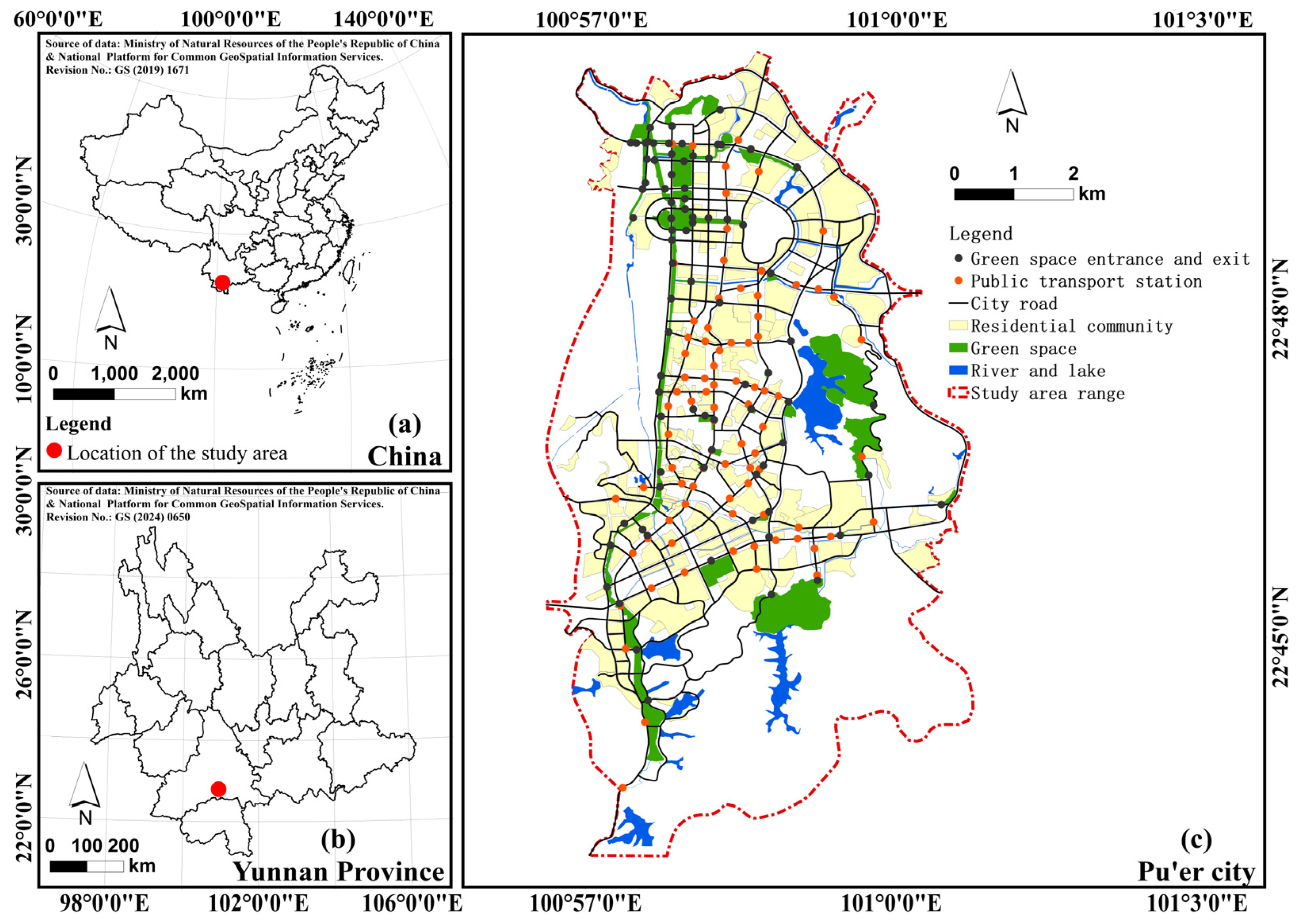
2.1.1. Overview of the Research Area

This study selects a category of green space with daily recreational function, open to the public, with certain recreational facilities and service facilities, as well as ecological soundness, landscape beautification, science popularization and education, and emergency evacuation as the object of accessibility optimization in Pu’er City, Yunnan Province, China, which is referred to as recreational green space (Figure 1). According to China’s Urban Green Space Classification Standard, parks (G1) and squares (G3) are included, while the scenic recreational green space (EG1) outside the urban construction land and away from the residential area is not taken into account. The study considers the potential link between park availability and utilization, calculates the service intensity of recreational green space based on the attractiveness of recreational green space based on the interaction model and network analysis method [36], and predicts the intensity of interaction between urban residents and recreational green space. By analyzing the spatial layout, actual use and supply level of recreational green spaces, the interaction intensity between urban residents and different recreational green spaces was compared to evaluate the accessibility of recreational green spaces. Optimization suggestions are made in two aspects: spatial layout of recreational green space and improvement of service quality of recreational green space, aiming to discover the spatial differences in recreational green space services, trying to avoid limiting factors, and searching for the most economical and feasible optimization strategy of recreational green space accessibility, in order to reduce the construction cost and save the use of land.
Pu’er City is the first national-level green economy pilot demonstration zone in China and was named a “National Garden City” in 2013. Considering the size, economic development status, and population of the city, Pu’er City is selected as a representative of small- and medium-sized cities and chosen as a case study. The scope of this study is consistent with the urban-planning area of Pu’er City, located in the central part of Simao District, Pu’er City, Yunnan Province. It is the area with the largest urban population and the highest level of urbanization in Pu’er City. According to the 2020 China Population Census Yearbook, by the end of 2020, the urban population in the urban-planning area was 289,662, with a total of 24,365 families, and the urbanization level was nearly 69.6%. The planning area was about 65.87 km2, and the built-up area was 26.5 km2. There were 34 recreational green spaces in the study area, with a total area of 4.28 km2.

2.1.2. Big Data of Mobile Geographic Location

In recent years, with the development of big data, which can continuously be able to continuously measure daily life activities through big data of mobile phone geolocation and big data of population distribution [37], a large number of researchers have associated life activities with various types of urban functions as a way to analyze various types of hotspot areas and resource needs [38]. Among the studies that used big data of cell phone geolocation to analyze green space functions, Jay et al. monitored visits to urban green spaces through big data of cell phone geolocation [39,40], and Filazzola et al. identified areas of high recreational green space use through activity density and activity coverage and performed correlation analysis on trail density; green space biological diversity patterns were correlated and analyzed [38]. In addition to analyzing the spatial distribution of people in green spaces through big data of cell phone geolocation, factors such as the time people visit green spaces and the factors affecting the visit time can also be analyzed through the big data of cell phone geolocation [41]. Therefore, in this study, using anonymous cell-phone-geolocation big data, the interaction between residents and recreational green space in the urban-planning area of Pu’er City, China, was investigated, the attractiveness of recreational green space and the supply level of urban recreational green space were calculated, a new interaction model was established from the perspective of the individual’s choice behavior, and the study was able to analyze the spatial layout situation and the utilization of the urban recreational green space at the same time.
This study uses a dynamic population location dataset provided by China’s Baidu Maps WiseEye platform for Saturday, June 12, 2020, from 7:00 to 19:00, which represents population dynamic population location data for a typical day off for urban residents. When residents use their cell phones or apps, the platform collects the user’s coordinates, time, and other data that have been cleaned, filtered, and removed from personal privacy information. The accuracy of the data is 200×200 m, and the user location information is recorded every hour. Considering that the platform only collects user location data when the cell phone or application is turned on and fails to collect dynamic population location data of urban residents at any time, the data results cannot yet reflect 100% of the travel behavior of all urban residents. Therefore, this limitation must be considered when using dynamic population location data for analysis [6]. This study superimposed the recreational green space boundaries with the dynamic population location data to characterize the commuting behavior of residents with cell-phone-positioning data [42]; users staying within the recreational green space were regarded as the actual users of the recreational green space, and each user had a unique ID. After that, the visit rate of the recreational green space was obtained by calculating the visit rate of the recreational green space in every hour interval, and the average visit rate of each piece of the recreational green space was obtained from 7:00 to 20:00. After that, the number of visitors to each recreational green space is obtained by combining the total population of the city, and the access level of each recreational green space is calculated.

2.1.3. Other Basic Data

This study downloads the satellite images of Pu’er City urban-planning area with a resolution of 0.55 m in June 2020 from Google Earth; obtains the location information of green areas, roads, waters, and construction sites based on the images; enters them into ArcGIS through vectorization tools; and obtains the data of public transportation stations in the planning area from the public transportation network of Pu’er City. Referring to the Pu’er City Urban Master Plan, Pu’er City Road Transportation Plan, Yunnan Provincial Population Census Yearbook, and the 2020 urban population data with residential neighborhoods as the statistical unit, a handheld GPS was used to conduct field visit surveys to supplement and correct the acquired information to obtain specific information on recreational green spaces, roads, public transportation stations, waters, and residential areas.

2.2. Method

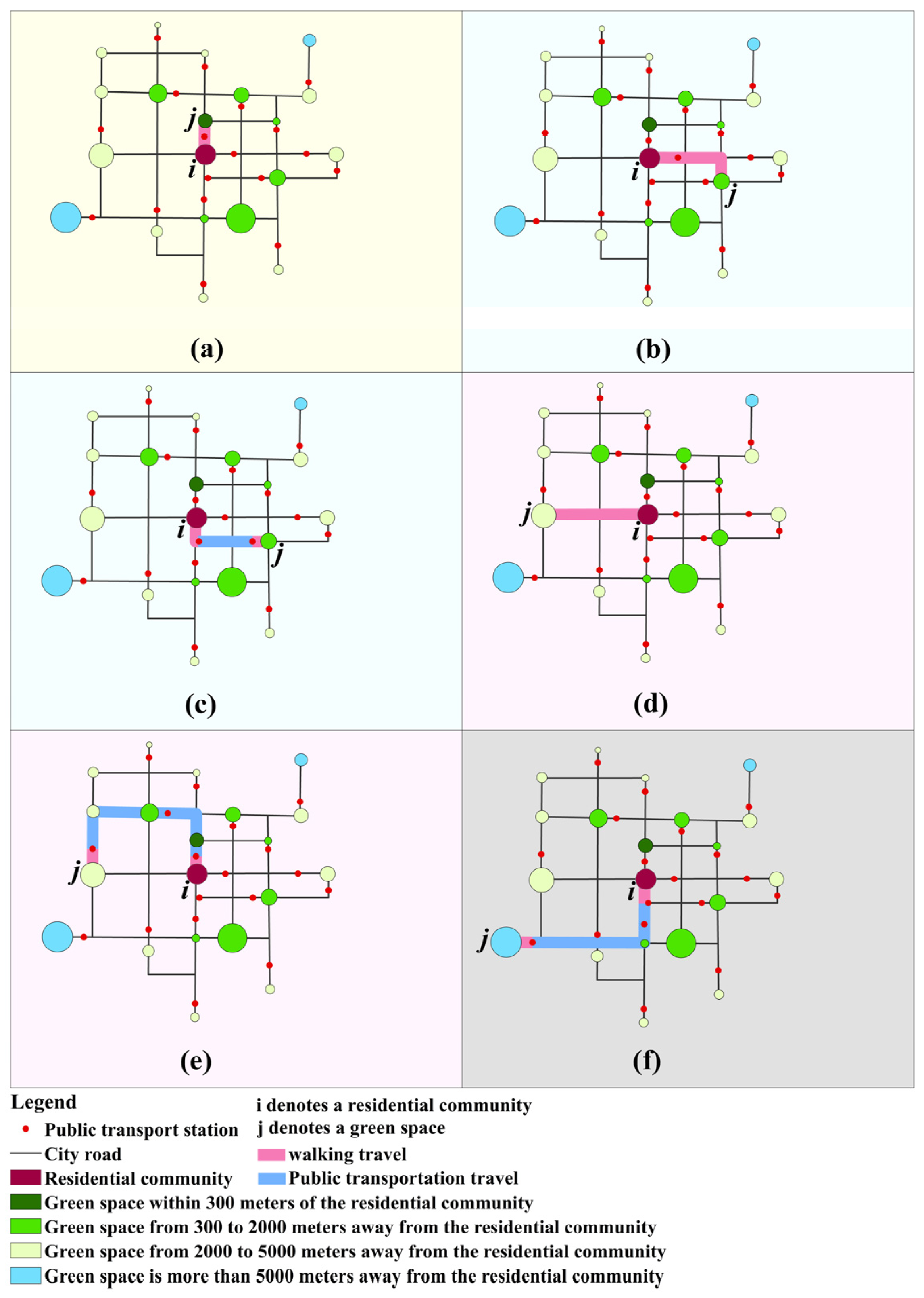
2.2.1. Construction of a Preferred Green Space Selection Model

The factors considered and models calculated in the study of green space accessibility are complex and varied, but this study is still in the process of researching which model is the most appropriate to measure the usage of green space and simulate the access of urban residents to green space. For this reason, this study compiled a list of relevant models for predicting population mobility. Commonly used models for predicting population movement include gravity model (also known as distance decay method) [43], radiation model [44], improved radiation model [45], population-weighted opportunity model (PWO) [46], opportunity priority selection model (OPS) [47], interactive city choice model (ICC) [48], and scaling law [49].
The gravity model can describe the interaction strength between two locations, which decreases with distance [6]. The gravity model is based on Newton’s law of gravity and is more applicable to the prediction of long-distance interactions, while the spatial choice behavior of individuals is less involved [50]. The use of the gravity model to predict the interaction between urban residents and green space lacks the consideration of individual spatial choice behavior and residents’ travel modes. The radial model or improved radial model assumes that individuals will only choose the nearest location that has a greater opportunity (benefit) than the departure location [48], which fails to capture the reality of short-distance elemental interactions [51].
PWO individuals’ choice of destination is directly proportional to the number of opportunities at the destination and inversely proportional to the total population of the location where the distance to the destination is shorter than or equal to the distance that residents have to travel from their origin to the destination [46]. OPS lack of consideration of the accessibility of the public transportation network will result in individuals choosing destinations where their maximal opportunity benefit is higher than that of their origin [47], and the city’s public transportation network is an important greenfield accessibility influence factor. The ICC model is subject to a fixed intercity transportation network; the higher the population of a city, the higher the intensity of its external interactions, and the higher the GDP of a city, the higher the intensity of its incoming interactions. On the other hand, under the premise that the population and GDP of all cities are fixed, and the travel time between cities is calculated by the shortest intercity travel time path in the transportation network, the higher the accessibility of a city in the intercity transportation network, the higher its interaction intensity [48]. However, the ICC, as used in modeling the intensity of interaction between urban settlements and green spaces, does not take into account the diversity of residents’ travel modes and habits and the complexity of calculating the shortest travel time in urban public transportation networks. For example, with the same travel distance, different modes of travel can result in differences in travel time and cost.
This study combed the related models and found that the OPS and ICC are mainly used to predict intra- or inter-city mobility due to employment opportunities, etc. OPS and ICC predict intra- or inter-city mobility by using distance and time as the cost of travel, and the prediction results of ICC are more in line with our subjective perceptions and can better reflect the urban population than the radiation model, GDP, and transportation network on inter-city people mobility [48]. In contrast, when measuring intra-city movement of people over short distances, the ICC does not consider the calculation of travel costs when combining multiple modes of travel and does not take into account the possible differences in road transportation accessibility in different areas of the city. Due to the age, psychological preference, behavioral preference, and other factors of urban residents, the residents’ travel modes are diversified. For example, following the same path to the same green space, young people travel to the green space by walking, and older people travel to the green space by taking public transportation, and they may spend different amounts of time and money. For the same distance, different travel modes may result in different time costs.
In order to reflect the difficulty for residents to reach recreational green spaces in different areas and to identify attractive and highly utilized recreational green spaces in the city, we established a model to measure the probability of green space use based on the urban public transportation system, named Preferred Selection of Green Spaces (PSG). The results of the PSG calculations are proportional to the attractiveness of the green space, the number of residents, and inversely proportional to the cost of the trip, as Equation (1) shows:
G i j = N i Q i j P i j = N i M i j S j I j T i j I j T i 1 + I j T i 2 + I j T i 3 + I j T i j + + I j T i n
In the equation of public notice (1), Gij is set as the intensity of interaction between residential area and recreational green space (the probability that the recreational green space is used), Ni is set as the number of residents in the residential area, Qij is set as the attractiveness of recreational green space j as a proportion of the attractiveness of all the recreational green spaces in the city, and Pij is set as the proportion of the cost of the trip spent by the residential area i to the recreational green space j as a proportion of the sum of the cost of the trip spent by the residential area i to all the recreational green spaces in the city. Mij is set to be the attractiveness of recreational green space j, Sj is set to be the sum of the attractiveness of all recreational green spaces in the city, Ij is set to be the sum of the travel costs from residential area i to all recreational green spaces, Tij is set to be the cost of travel from residential area i to recreational green space j, and Tin is set to be the cost of travel from residential area i to recreational green space n. It is important to note that the intensity of interaction between residential areas and recreational green spaces, Gij, is not an actual flow rate but a dimensionless value reflecting the tendency or probability of residents to choose to use recreational green spaces.
Network analysis is an effective tool for the analysis of human flow, water flow, traffic flow, etc. Its elements include center, link, node, and impedance [8]. The network analysis method based on roads can more realistically reflect the process of residents arriving at recreational green spaces and can more accurately and objectively analyze the accessibility of recreational green spaces. Using ArcGIS technology to establish the road network analysis model, in order to more realistically reflect the actual arrival of people in different directions to their destinations, the entrance/exit of the recreational green spaces is defined as the center of the network analysis; the link is a city road, the node is a road intersection, the impedance is the waiting time at traffic intersections, set as the average waiting time at each intersection is 0.5 min; the average speed of people walking is 1.25 m/s [42], and the average speed of buses is 9.28 m/s [52].

2.2.2. Calculation of the Attractiveness of Recreational Green Spaces

There are many factors affecting residents’ choice to use recreational green spaces. On the one hand, they are related to the landscape quality, service facilities, area size, and management level of the recreational green spaces themselves. On the other hand, it is related to the type of recreational green spaces users, residential location, psychological preference, behavioral preference, etc. There are many factors involved, and it is difficult to measure the weight of indicators. In this study, the attractiveness of recreational green spaces is measured directly through the results of actual use of recreational green spaces, and the more people use recreational green spaces per unit area and the longer the time, the higher the attractiveness of recreational green spaces [53]. In addition to reflecting the attractiveness of recreational green spaces, the results of the actual use of recreational green spaces can also measure the supply level of recreational green spaces and the trip rate of urban residents.
In this study, we refer to the Accessible Natural Greenspace Standards of the United Kingdom and classify the recreational green spaces into city level (area ≥ 100 hm2), regional level (area ≥ 20 hm2 > 100 hm2), and community level (area > 20 hm2) according to the size of the recreational green spaces [54]. The per capita land index is based on the “capacity calculation” stipulated in the “Code for the design of public park” (GB 51192-2016) implemented in China, and it is set so that the per capita land area of recreational green spaces at the city level and regional level is 60 m2, the per capita water area is 250 m2, the per capita land area of recreational green spaces at the community level is 30 m2, the per capita area of recreational green spaces is 30 m2, and the per capita area of recreational green spaces is 30 m2 [55]. This study used the visit level of recreational green spaces to represent the attractiveness of recreational green spaces and compared the number of visitors to recreational green spaces with the population capacity of the green spaces to calculate the attractiveness of each recreational green space in the urban-planning area of Pu’er City, and the calculation equations were as shown in Equations (2)–(6):
F =   Sample   Number   Of   Visitors   green   space × Total   Population   city Sample   Number   Of   Visitors   city  
C = A A m = C c i t y + C c o m m u n i t y
C city = A l a n d 60 + A w a t e r 250
C community = A l a n d 30 + A w a t e r 150
M = F C = F × A m A = F C c i t y + C c o m m u n i t y
In the Equation, F represents the number of residents using recreational green space in the city, Sample Number Of Visitorsgreen space represents the number of residents using recreational green space among those who have turned on cell phone location positioning, Total Populationcity represents the total number of residents in the city, Sample Number Of Vistorscity represents the total number of residents who have turned on cell phone location positioning, C represents the population capacity of recreational green space, Ccity represents the population capacity of recreational green space at the city level and the regional level, Ccommunity represents the population capacity of recreational green space at the community level, A represents the area of recreational green space, Am represents the per capita area of recreational green space, Aland represents the land area of recreational green space, Awater represents the water area of recreational green space, and M represents the attractiveness of recreational green space.

2.2.3. Calculation of Travel Costs

The real travel cost of residents is an important basis for calculating the interaction intensity of recreational green spaces. Travel cost is generally measured by travel distance, travel time [56], and the cost incurred by the travel [57]. However, short-distance trips by intra-city residents have significantly different travel modes compared to long-distance, inter-city trips. While long-distance, inter-city trips are typically made via automobile and other modes of transportation, short-distance trips by intra-city residents consist of walking, automobile trips, and public transportation trips. This is coupled with individual economic differences among residents, the insensitivity of some residents to the costs incurred for traveling, and the costs not directly incurred by residents walking. In summary, it was found that factors such as the urban transportation network, the distribution of public transportation stops, and the mode of travel must be taken into account when using geographic distance and time to measure the cost of residents’ trips to recreational green spaces [58] because trips need to pass through the urban transportation network regardless of the mode of travel, and the cost of trips cannot be measured simply by calculating the geographic distance between the residential area and the recreational green space [59], as shown in Figure 2a,b. In addition, because the distance of travel has a great influence on the mode that residents choose to travel [20], this study calculates and grades the distance between residential areas and all recreational green spaces based on the urban public transportation network and determines the travel modes that residents may use based on the distance, as shown in Figure 2c.
In order to cope with climate change and respond to the call for green and low-carbon travel, the travel modes of inner-city residents to recreational green spaces in this study refer to the survey and research results of Fan et al. [20], i.e., urban residents go to recreational green spaces within 300 m from residential areas all by walking; to recreational green spaces beyond 300 m and within 2000 m from residential areas, 50% would be on foot and 50% by public transportation; 25% of the recreational green spaces beyond 2000 m and within 5000 m from the residential area are accessed by walking and 75% by public transportation; 100% of the recreational green spaces beyond 5000 m from the residential area are accessed by public transportation, as shown in Figure 3. This study establishes a travel cost matrix between residential communities and recreational green spaces through a network analysis model, taking the geometric center of the residential area as the starting point, the geometric center of the recreational green space and the public transport stops as the destination points, and the shortest plumb line from the starting point to the road as the “connection”, and calculates the actual shortest travel cost from the geometric center of the residential area to the geometric center of the recreational green space of different levels and to the nearest public transport stops. Using the shortest vertical line from the starting point to the road as the “connection”, the actual shortest paths from the geometric center of the residential area to the geometric center of the different levels of recreational green space and the nearest public transportation station are calculated.
The travel time to reach the recreational green space within 300 m from the residential area is calculated as shown in Equation (7):
T j 300 = dist j 300 1.25
In Equation (7), Tj300 is set as the travel time from residents of the residential area to the recreational green space within 300 m from the residential area, distj300 is set as the shortest distance from the geometric center of the residential area to the geometric center of the recreational green space within 300 m from the residential area, and the average walking speed is set as 1.25 m/s.
The travel time calculations for reaching recreational green spaces beyond 300 m and within 2000 m from residential areas are shown in Equations (8)–(10):
T j 2000 = 1 2 × Walking j 2000 + 1 2 × PT j 2000
Walking j 2000 = dist j 2000 1.25
PT j 2000 = dist min   1.25 + dist j 2000   dist min 9.28
In this Equation, Tj2000 is set as the travel time of residents of the residential area to the recreational green space that is 300 m away from the residential area and 2000 m and less, which consists of the walking-travel time (Walkingj2000) and the public transportation travel time (PTj2000). Distj2000 is set as the shortest distance from the geometric center of the residential area to the geometric center of the recreational green space that is 300 m away from the residential area and within 2000 m, distmin is set as the shortest distance from the geometric center of the residential area to the nearest public transportation station, and the average speed of the vehicle is set as 9.28 m/s.
The travel time calculation equations for reaching recreational green spaces beyond 2000 m and within 5000 m from residential areas are shown in Equations (11)–(13):
T j 5000 = 1 4 × Walking j 5000 + 3 4 × PT j 5000
Walking j 5000 = dist j 5000 1.25
PT j 5000 = dist min   1.25 + dist j 5000   dist min 9.28
In this Equation, Tj5000 is set as the travel cost for residents of the residential area to the recreational green space beyond 2000 m and within 5000 m from the residential area, which consists of the walking-travel cost (Walkingj5000) and the public transportation travel cost (PTj5000). distj5000 is set as the shortest distance from the geometric center of the residential area to the geometric center of the recreational green space within 5000 m from the residential area, and distmin is set as the shortest distance from the geometric center of the residential area to the nearest public transportation stop.
The Equation for calculating the travel time to reach an recreational green space beyond 5000 m from a recreational area is shown in Equation (14):
T j 5000 p = dist j 5000 p 9.28
In this Equation, Tj5000p is set as the travel time from the residents of the residential area to the recreational green space 5000 m away from the residential area. distj5000p is set as the shortest distance from the geometric center of the residential area to the geometric center of the recreational green space 5000 m away from the residential area.
The travel time spent by settlement i to all the recreational green spaces in the city is summed up to obtain the sum of travel time Ij for settlement i. The Equation for calculating the sum of travel time of residents is shown in Equation (15):
I j = T j 300 + T j 2000 + T j 5000 + T j 5000 p

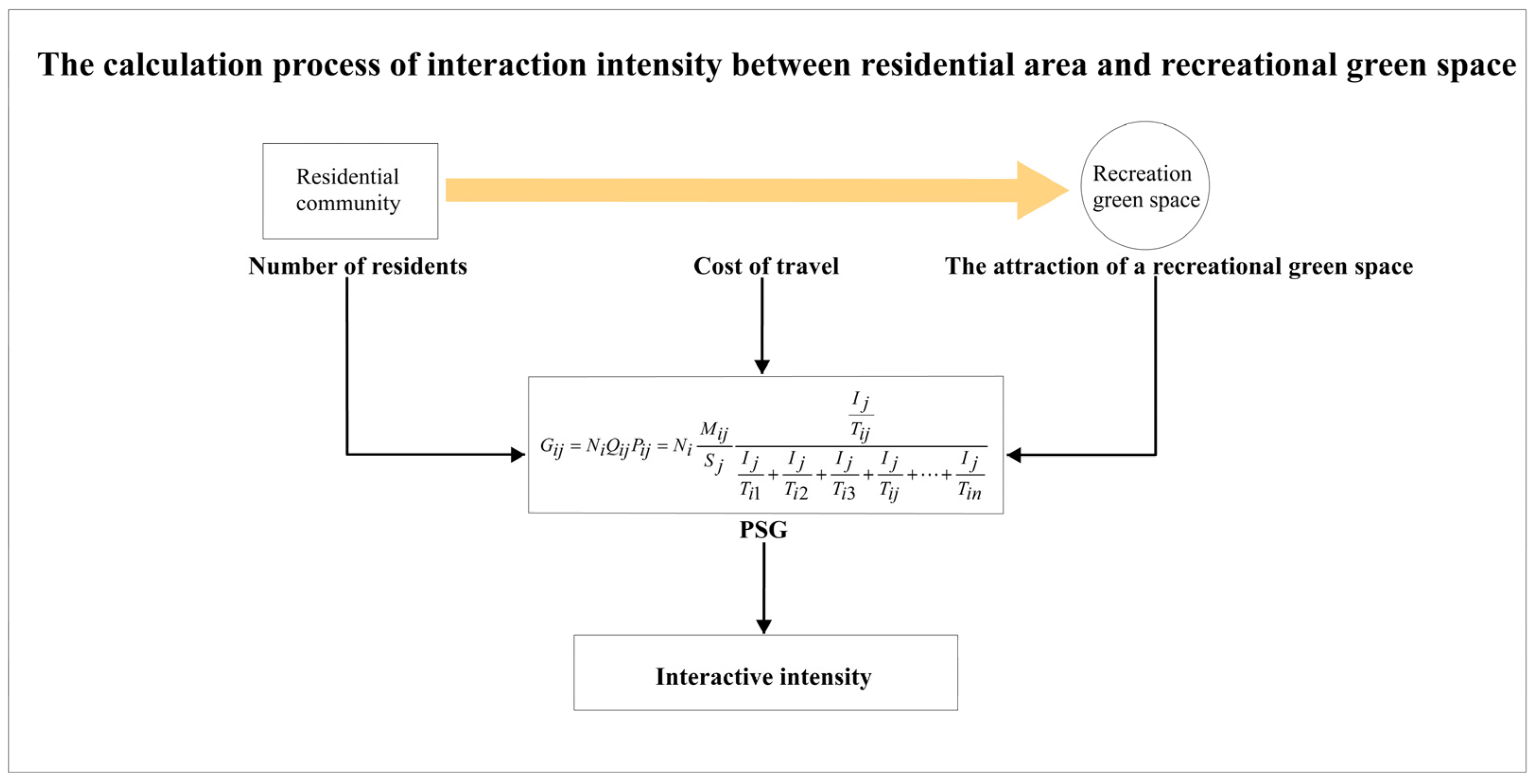
2.2.4. Calculation of the Intensity of the Interaction

PSG was used to calculate the interaction intensity between urban residential areas and recreational green spaces in Pu’er City on the June 2020 rest day. Firstly, the population number in the residential areas is obtained; then, the travel cost is calculated based on the shortest path from residential areas to each recreational green space, and finally, the interaction intensity of recreational green space is calculated based on Equation (1) by combining the attractiveness of recreational green space. The calculation process is shown in Figure 4:

3. Results and Analysis

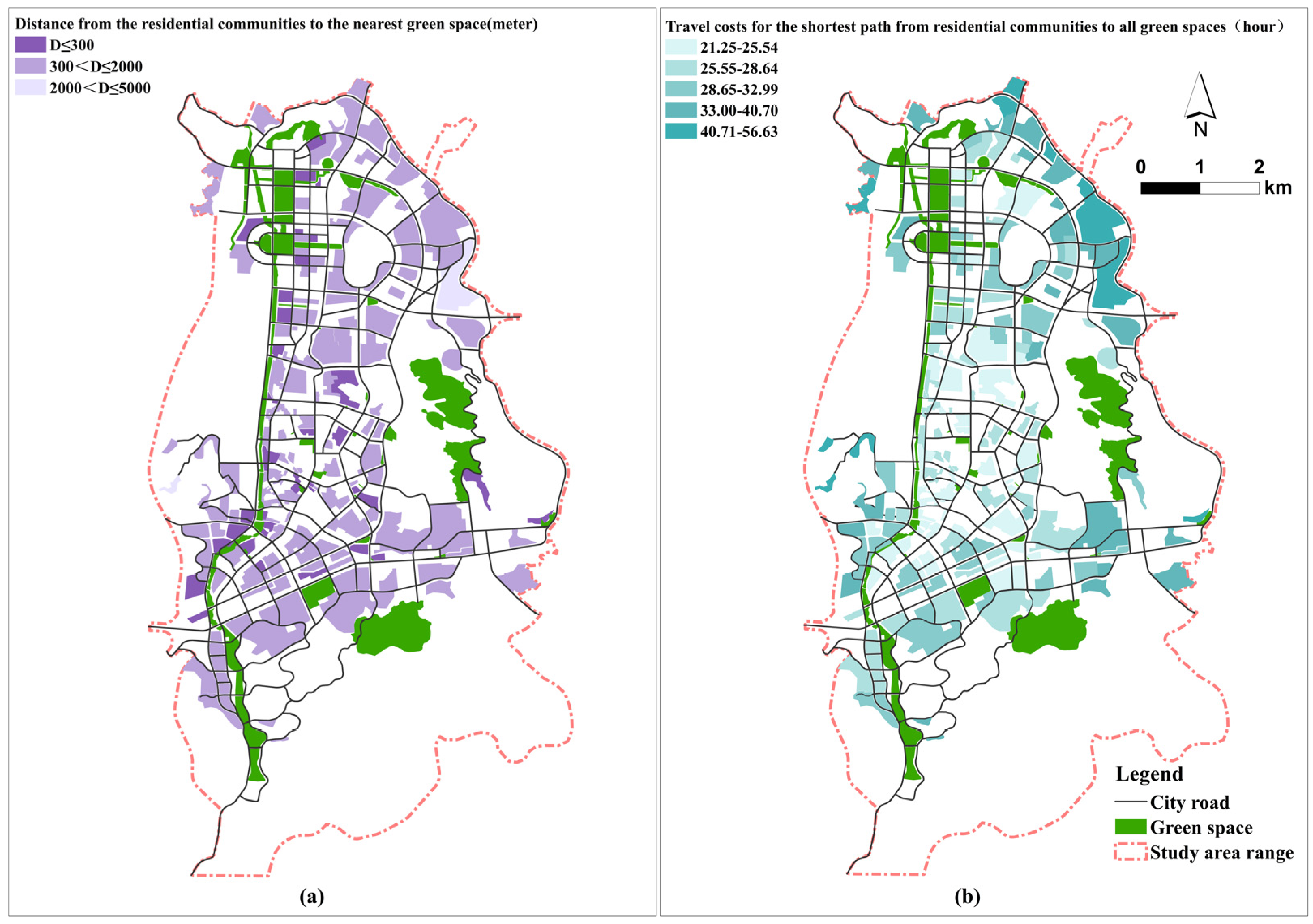
3.1. Spatial Layout Analysis

As shown in the previous Section 2.1.1., urban recreational green space and public transportation facilities in Pu’er City show obvious spatial aggregation, with significant differences in horizontal spatial distribution. In the eastern, southeastern, and northwestern parts of the urban-planning area, large areas of recreational green space are distributed, while in the central part of the city, recreational green space is smaller and less distributed. The road network and public transportation stations in the central part of the urban-planning area are densely distributed, while the road network in the eastern, western, southwestern, and northeastern parts of the urban-planning area is sparse, and there are fewer public transportation stations.
This study conducted a field survey on the population size of each residential area in Pu’er City and drew a map of the spatial distribution of the population in the urban residential areas based on the survey data (Figure 5a). From the point of view of the spatial distribution of the population, there is a large difference in the population size of the residential areas in Pu’er City, and the urban population is mainly located in the central, southwestern, and northeastern residential areas of the city. This results in a relatively high population density in the central, southwestern, and northeastern parts of the city, and the distribution of the urban population shows a clear state of aggregation.
According to Equation (1), the number of real-time visitors to the recreational green space from 7:00 to 19:00 on 12 June 2020 (Saturday) was obtained by combining the real-time location data of cell phones and the total population data of the city (Figure 5b). The results show that the actual number of visitors to recreational green spaces in the central part of Pu’er City, which is easily accessible by public transportation, and those with a larger area at the edge of the city are higher. This implies that in actual use, people may tend to use recreational green spaces that are closer to residential areas, easily accessible by public transportation, or larger in size.
This study calculated the theoretical population capacity of different classes of recreational green space based on the per capita green space area (Figure 6a) and graded the theoretical population capacity of recreational green space. The results showed that the recreational green space with higher population capacity was mainly distributed in the urban fringe, while the central part of the city, where the distribution of residential districts was dense, had a generally smaller population capacity due to spatial constraints, etc. This study also found that the recreational green space with higher population capacity was mainly located in the urban fringe, while the central part of the city, where the distribution of residential districts was dense, had a generally smaller population capacity due to spatial constraints.
This study assessed the attractiveness of recreational green spaces based on the theoretical population capacity of the recreational green spaces and the actual number of users of the recreational green spaces (Figure 6b), with the attractiveness of the recreational green spaces reflecting the service quality or supply and demand of the recreational green spaces, as shown in Figure 6c. Circles represent recreational green spaces, with bright colors indicating the greater attractiveness of recreational green spaces. In terms of spatial distribution, the more-attractive recreational green spaces are mainly distributed in the central, southwestern, and northern parts of the urban-planning area. These recreational green spaces are generally close to residential areas and are densely surrounded by public transportation facilities, so the actual number of users exceeds the designed population capacity, and the number of users per unit area is high. This implies that the more attractive recreational green spaces may have higher service quality and more residents are willing to visit them for recreational activities, which also results in the supply of this part of recreational green spaces being less than the demand. The less attractive recreational green spaces are mainly located in the southern and eastern parts of the city. The residential areas and public transportation facilities around these recreational green spaces are less distributed, and the actual number of users is far less than the designed population capacity, which results in the supply of recreational green spaces far exceeding the demand.

3.2. Analysis of Travel Costs

The network analysis model was used to establish the cost matrix between recreational green spaces and residential communities, and the study counted the number of people who could be reached by different distance classes (Table 1) and the sum of travel costs for residents of residential areas to all recreational green spaces (Table 2) to generate the distance grading map from residential areas to the nearest recreational green space (Figure 7a) and the shortest path travel cost grading map from residential areas to all recreational green spaces (Figure 7b). The analysis of the distances from residential areas to the nearest recreational green space shows that in terms of the number of residential areas, 19.91% of the residential areas are not more than 300 m away from the nearest recreational green space, and 99.1% are not more than 2000 m away from the nearest recreational green space. In terms of the proportion of population, 99.14% of the residents of the residential areas can reach the nearest recreational green space at a relatively small cost, while only 0.86% of the residents of the residential areas located in the eastern and western fringes of the city need to spend more to reach the nearest recreational green space. This indicates that under the current urban transportation network, most of the residents in the residential areas can reach the recreational green space quickly by walking, according to the principle of proximity.
Based on the total travel cost of the shortest route to all recreational green spaces for residents of residential areas, the results show that under the combination of walking and public transportation, the total travel cost of the shortest route to all recreational green spaces for residents of 60.17% of the residential areas, which are mainly located in the central, southwestern, and northern parts of the city, ranged from 21.25 h to 28.33 h. These locations generally have lower travel costs for residential areas in the central, southwestern, and northern portions of the city due to the dense urban roadway network and the concentration of community-level recreational green space and public transportation stops. In total, 1.02% of residential areas have a combined travel cost of 49.56 to 56.63 h for the shortest route to all recreational green space, and these residential areas are primarily located in the northeastern portion of the city, where there is a sparse amount of recreational green space and public transportation stops. The results show that the shortest paths in Pu’er city are mainly located in the northeastern part of the city. The results show that the spatial layout of urban recreational green spaces and public transportation stations in Pu’er City is generally reasonable, and the sum of travel costs of the shortest paths from most of the residential districts to the recreational green spaces is kept at a relatively low level, but there are some residential districts in which the travel costs are larger due to the irrational layout of the recreational green spaces and public transportation stations. The next step can be to optimize the spatial layout of recreational green spaces, urban transport networks, or public transport stations according to the specific land use conditions, so as to reduce the travel costs from residential areas to recreational green spaces.

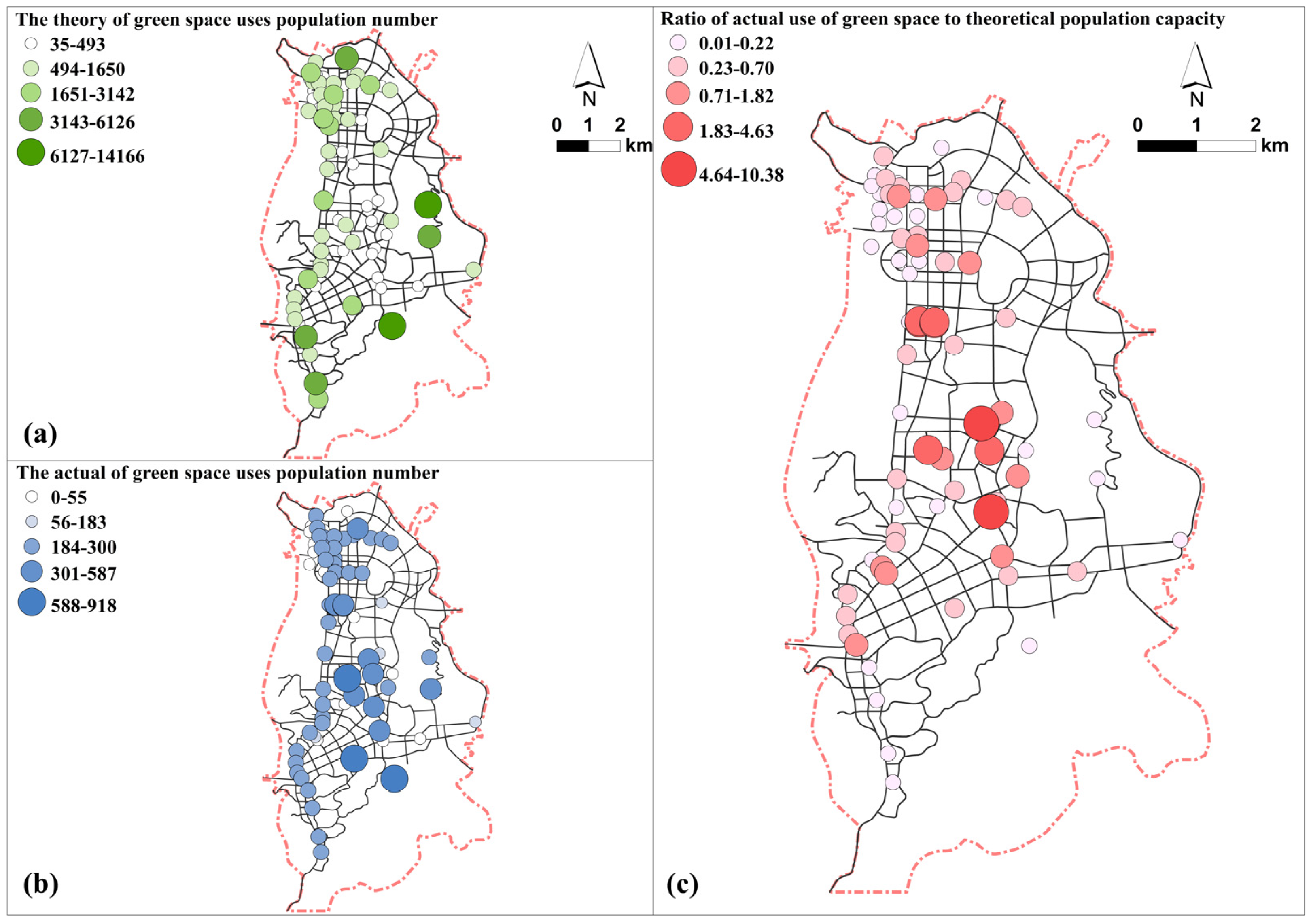
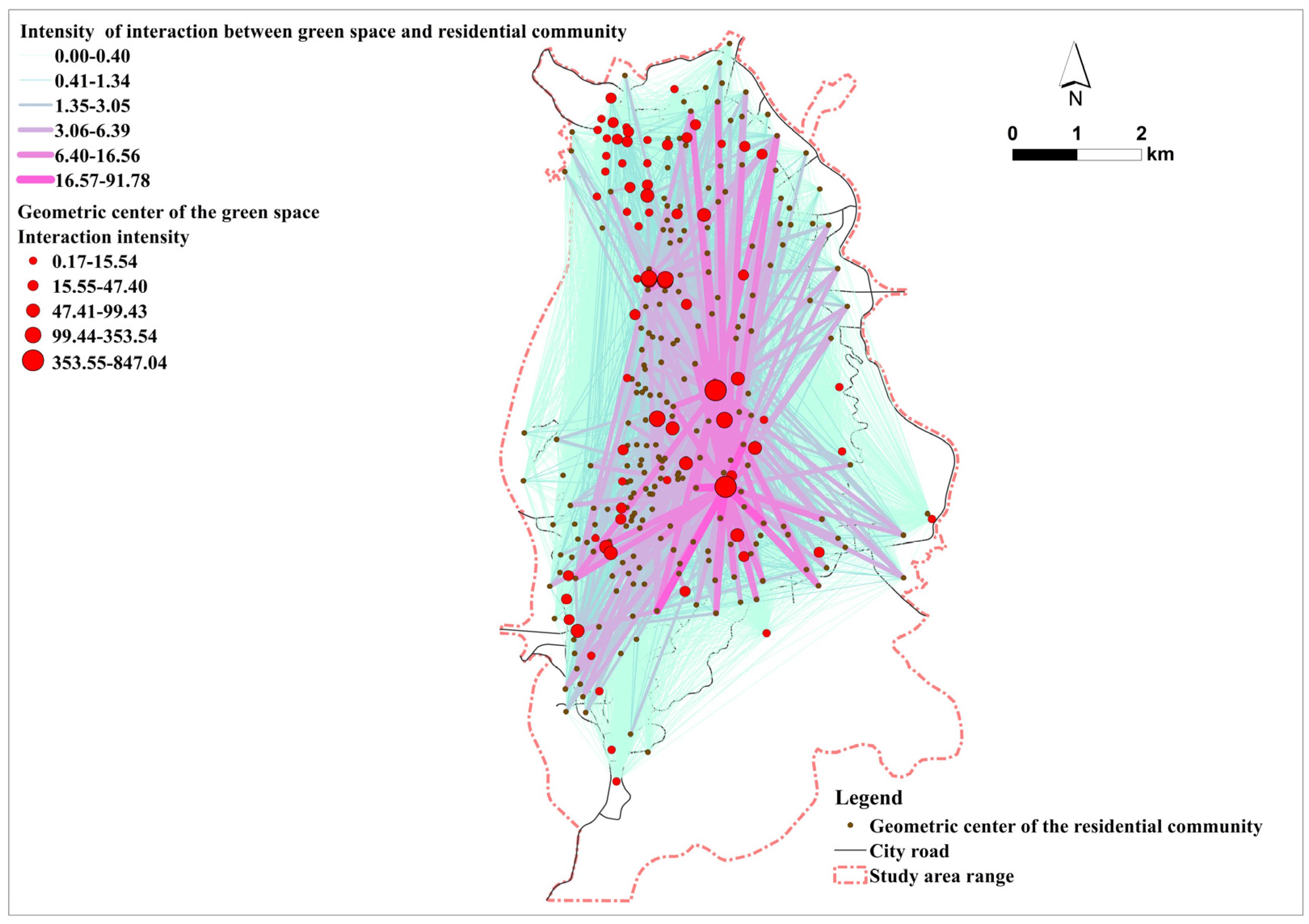
3.3. Recreational Green Space Utilization Analysis

The results of the calculation of the interaction intensity between urban residential areas and recreational green spaces in Pu’er City are shown in Figure 8, which shows that the probability of recreational green spaces in the central, southwestern, and northern parts of the city being used is higher than that of recreational green spaces in the eastern and western parts of the city. This suggests that urban residents may prefer to use recreational green spaces that are closer to residential areas and more attractive. The probability of using recreational green spaces at the edge of the city, farther away from most of the residential areas, and surrounded by few public transportation facilities is lower.
This study calculated a Gini coefficient of 0.69 for the interaction intensity of recreational green spaces in Pu’er City based on the interaction intensity of recreational green spaces and found that the utilization of recreational green spaces in Pu’er City is polarized. A part of the recreational green space with low utilization rate is distributed at the edge of the city. Although this part of the recreational green space is larger in size, it has a lower probability of being chosen by residents due to its distance from residential areas and poor accessibility to public transportation (fewer public transportation stops and fewer road distributions near the recreational green space). The other part of recreational green space with lower interaction intensity is located near residential areas. This part of the recreational green space has a smaller population capacity and poorer green space service quality, which causes residents in this area to be willing to actively increase the cost of traveling to choose a recreational green space that is farther away and has better service quality.
The proportion of recreational green spaces with higher utilization rates is lower. These recreational green spaces with higher utilization rates are generally close to residential areas, and most of them are community-level recreational green spaces located in the central part of the city, which have better accessibility by public transport, better quality of green space services, and higher attractiveness of the green spaces themselves. However, these highly utilized recreational green spaces are not able to serve the majority of the city’s residents due to their small population capacity. In actual use, this may cause some residents to passively increase their travel costs and choose farther and larger recreational green spaces due to congestion and other reasons. When this happens, it is necessary for urban planners or government workers to optimize the spatial layout of the recreational green space in the area or to improve the accessibility of public transport in order to meet the needs of the residents in the area or to reduce the travel costs of the residents in the area.
The results of this study show that recreational green spaces that are highly accessible by public transportation and larger in size are used by more people in the city, which is consistent with the results of most studies. However, the most accessible recreational green spaces are not always the most used, which is inconsistent with the default assumption in the context of spatial equality. This is because this study considered the impact of the attractiveness of the recreational green space itself on residents’ choice of recreational green space. This study concluded that residents’ choice to use recreational green space is determined by a combination of travel costs and the attractiveness of the recreational green space. Some of the recreational green spaces are closer to residential areas, but they are smaller in scale, lower in population capacity and attractiveness, and cannot provide residents with abundant activity space and high-quality recreational services, resulting in a lower probability of being chosen by residents. The probability of residents choosing to use recreational green space is the highest for green spaces that are closer to residential areas and have a larger population capacity and higher attractiveness.
Overall, due to differences in population distribution among urban residents, varying attractiveness of recreational green spaces, and uneven spatial layout of public transportation facilities, some residents are still unable to fully and equally access urban recreational green spaces and enjoy the services they provide. In order to have equal access to urban recreational green spaces and enjoy the services brought by recreational green spaces, firstly, it is possible to consider reducing the travel costs of residential areas on the outskirts of the city, improving the public transportation facilities near these residential areas, creating new environmentally friendly transportation networks or improving the accessibility of public transportation, so that the travel costs of all residential areas remain at the same level. Secondly, consider recreational green spaces with high utilization rates but small population capacity. By improving the ecological benefits and service quality of recreational green spaces through landscape design, more activity spaces can be created to meet the leisure and recreational needs of residents. Finally, the population distribution of urban residents, the attractiveness of recreational green spaces, and the accessibility of public transportation affect the utilization rate of recreational green spaces. In the future, when updating and renovating urban recreational green spaces, we need to comprehensively consider these influencing factors and then improve the accessibility and utilization rate of recreational green spaces in the most economical and convenient way.

4. Discussion

4.1. Advantages of PSG

In order to make the utilization of recreational green spaces more equitable, it is crucial to assess the spatial distribution and service quality of existing urban recreational green spaces [60,61]. This study developed a model to measure the probability of green space use (PSG) from the perspective of individual choice. The model uses the ratio of the average number of users to the theoretical capacity of the recreational green space to represent the attractiveness of the green space, the shortest path in the urban public transportation network to calculate the cost of residents’ travel on foot and by public transportation, and the number of residents in the residential area to represent the number of choices made by the residents. The PSG integrates the attractiveness of the recreational green space, the residents’ travel preference, the distribution of the permanent population, and other key factors affecting the accessibility of the green space, which can visualize residents’ use of recreational green spaces, and is conducive to identifying the most popular recreational green spaces in the city and discovering residential areas with higher travel costs.
To demonstrate the advantages of PSG, this paper measures the intensity of interaction between residential areas and recreational green spaces in Pu’er, China. The attractiveness and supply level of recreational green spaces in Pu’er were assessed using big data on the geographic location of cell phones, revealing inequalities in the use of recreational green spaces due to differences in the size and attractiveness of the recreational green spaces themselves, as well as differences in the distribution of public transportation facilities in the city, and differences in the distribution of the city’s population, which provide guidelines for refining the layout of the recreational green spaces and improving the public transportation facilities in the city of Pu’er. At the same time, PSG provides a method for measuring the movement of people between residential areas and green spaces within the city, and through improvement, it can also be applied to the measurement of interactions between other factors within the city, which provides new perspectives and valuable references for the planning of urban infrastructure [62,63], and is of great significance for the sustainable development of urban green spaces.

4.2. Limitations of PSG

Although PSG is able to obtain reasonable results in measuring the intensity of interaction between residential areas and recreational green spaces, there is still room for expansion in practical applications. In this study, the results of the actual use of recreational green spaces were obtained through big data of cell phone geolocation as a way to reveal residents’ preferences for use of recreational green spaces [6,64], and the attractiveness of recreational green spaces was reflected by the ratio of the actual average number of users of the recreational green spaces to the theoretical number of people they can accommodate [65]. This approach transgresses the complex investigation and assessment of the attractiveness or service quality of recreational green spaces and avoids the errors caused by the subjective factors of the assessors. However, the choice of recreational green spaces and the number of choices made by urban residents are not fixed; personal habits, seasonal changes, festivals, and working hours all affect the choice of recreational green spaces [66]. In the future, real-time location data with higher accuracy and longer time series can be used to measure the attractiveness of recreational green spaces.
Studies have shown that using public transportation for travel reduces travel time to recreational green spaces for all residents, and that differences in the accessibility and connectivity of public transportation affect residents’ use of recreational green spaces [67,68]. This time, in the travel time calculation, we assumed that all people have the same sensitivity to distance, did not consider the distance decay effect to bring about an impact [35], and directly calculated the travel time of residents through the cost-weighting method. In addition, the travel mode of residents in this study only includes walking and public transportation trips and does not involve mixed modes of travel [11], and the calculation of the cost of residential travel can be further improved. This study measured the accessibility of urban parks from the perspective of adult travel, and did not consider the travel ability and mobility patterns of children, the elderly, and tourists [10,69, 70], and the fairness of special groups’ access to recreational green space and utilization of available green space needs to be further measured [60], as a way of conforming to the mobility patterns of people from special groups and meeting their specific needs.

5. Conclusions

Climate change has become the world’s most important environmental issue, and mitigating and responding to climate change is one of the most pressing social and health challenges of our time. While climate change is a global issue, its impacts are very real and concrete. Promoting environmental justice is one of the powerful measures to mitigate and respond to climate change while also contributing to equitable access to health and socialization opportunities for individuals and communities. In order to reflect the ease of access to recreational green spaces in different areas, to identify attractive and well-utilized recreational green spaces in the city and to enable more residents to have easy access to high-quality recreational green spaces, this study introduces a new model for measuring the probability of use of recreational green spaces (PSG), which reveals the inequalities in the use of green spaces in the city.
The results of this study confirm that urban residents tend to use recreational green spaces that are closer to their residential areas and easily accessible or larger in scale, and that more residents are willing to carry out activities in more attractive recreational green spaces. However, due to the influence of the attractiveness of recreational green spaces, the utilization rates of some recreational green spaces which are closer to residential areas but less attractive and some recreational green spaces with a larger population capacity but less attractive are lower, which has led to the emergence of a special situation whereby the most easily accessible recreational green spaces and those of the largest scale may not always be the ones that are used the most or most frequently. This is also a reminder of the need to consider both transportation accessibility and attractiveness of recreational green spaces when promoting equitable access to health and socialization opportunities for individuals and communities. In addition, due to the uneven distribution of population in the city, when assessing the supply and demand of urban recreational green spaces, it is necessary to satisfy the balance of supply and demand for recreational green spaces in localized areas of the city, in addition to the balance of supply and demand for recreational green spaces at the level of the city as a whole.
Our study provides some valid insights for promoting equitable use of green spaces and enhancing the well-being of urban residents. However, the results of this study can be further improved due to the accuracy limitations of the cell phone geolocation data used for the study and the failure to include all possible travel modes of residents to green spaces. Future research could consider obtaining information such as type and age of residents from cell phone geolocation big data. At the same time, this study analyzes real-time location data over a longer time series, taking into account the differences in travel mode choices of different types of residents and their sensitivity to travel costs, and summarizes the patterns and preferences of different types of residents’ use of green space. In addition to grasping the current patterns and preferences of residents’ utilization of green space, it is also necessary to consider the impact of future climate change and economic development on the preferences and needs of residents, and it is necessary to carry out the design of green space according to the new needs of residents, so as to mitigate and respond to climate change.

Author Contributions

C.X.: Conceptualization, data curation, formal analysis, software, funding acquisition, visualization, writing—original draft, writing—review and editing. J.Z.: investigation, methodology, writing—original draft, writing—review and editing, methodology. Y.X.: investigation, supervision, visualization. Z.W.: funding acquisition, methodology, project administration, supervision, writing—review and editing. All authors have read and agreed to the published version of the manuscript.

Funding

This research has received funding from the “Xingdian Yingcai” Young Top-notch Program (YNWR-QNBJ-2020-104) and the Chuxiong Normal University School-level Research Team Project (XJTDB03).

Data Availability Statement

The data is available on request from the corresponding author.

Acknowledgments

We would like to express our sincere gratitude to all editors, reviewers, and staff who participated in the review of this article. The raw data supporting the conclusions of this article will be made available by the authors on request.

Conflicts of Interest

The authors declare no conflicts of interest.

References

  1. Team, U.-H.C. World Cities Report 2022. 2022. Available online: https://unhabitat.org/wcr/ (accessed on 28 October 2024).
  2. Khaza, M.K.B.; Rahman, M.M.; Harun, F.; Roy, T.K. Accessibility and service quality of public parks in Khulna city. J. Urban Plan. Dev. 2020, 146, 04020024. [Google Scholar] [CrossRef]
  3. Guo, R.; Diehl, J.A.; Zhang, R.; Wang, H. Spatial equity of urban parks from the perspective of recreational opportunities and recreational environment quality: A case study in Singapore. Landsc. Urban Plan. 2024, 247, 105065. [Google Scholar] [CrossRef]
  4. Gao, S.; Zhai, W.; Fu, X. Green space justice amid COVID-19: Unequal access to public green space across American neighborhoods. Front. Public Health 2023, 11, 1055720. [Google Scholar] [CrossRef]
  5. Li, H.; Ta, N.; Yu, B.; Wu, J. Are the accessibility and facility environment of parks associated with mental health? A comparative analysis based on residential areas and workplaces. Landsc. Urban Plan. 2023, 237, 104807. [Google Scholar] [CrossRef]
  6. Colbert, J.; Chuang, I.T.; Sila-Nowicka, K. Measuring spatial inequality of urban park accessibility and utilisation: A case study of public housing developments in Auckland, New Zealand. Landsc. Urban Plan. 2024, 247, 105070. [Google Scholar] [CrossRef]
  7. Rodrigues Ferreira Barbosa, V.; Maria Damasceno, R.; Andreotti Dias, M.; Castelhano, F.J.; Roig, H.L.; Requia, W.J. Ecosystem services provided by green areas and their implications for human health in Brazil. Ecol. Indic. 2024, 161, 111975. [Google Scholar] [CrossRef]
  8. Oh, K.; Jeong, S. Assessing the spatial distribution of urban parks using GIS. Landsc. Urban Plan. 2007, 82, 25–32. [Google Scholar] [CrossRef]
  9. Kong, F.; Yin, H.; Nakagoshi, N. Using GIS and landscape metrics in the hedonic price modeling of the amenity value of urban green space: A case study in Jinan City, China. Landsc. Urban Plan. 2007, 79, 240–252. [Google Scholar] [CrossRef]
  10. Guo, S.; Song, C.; Pei, T.; Liu, Y.; Ma, T.; Du, Y.; Chen, J.; Fan, Z.; Tang, X.; Peng, Y.; et al. Accessibility to urban parks for elderly residents: Perspectives from mobile phone data. Landsc. Urban Plan. 2019, 191, 103642. [Google Scholar] [CrossRef]
  11. Wang, S.; Wang, M.; Liu, Y. Access to urban parks: Comparing spatial accessibility measures using three GIS-based approaches. Comput. Environ. Urban Syst. 2021, 90, 101713. [Google Scholar] [CrossRef]
  12. Stoia, N.L.; Nita, M.R.; Popa, A.M.; Iojă, I.C. The green walk—An analysis for evaluating the accessibility of urban green spaces. Urban For. Urban Green. 2022, 75, 127685. [Google Scholar] [CrossRef]
  13. Mohamed, A.A.; Kronenberg, J.; Laszkiewicz, E. Transport infrastructure modifications and accessibility to public parks in Greater Cairo. Urban For. Urban Green. 2022, 73, 127599. [Google Scholar] [CrossRef]
  14. Shi, M.; Chen, M.; Jia, W.; Du, C.; Wang, Y. Cooling effect and cooling accessibility of urban parks during hot summers in China’s largest sustainability experiment. Sustain. Cities Soc. 2023, 93, 104519. [Google Scholar] [CrossRef]
  15. Zong, W.; Qin, L.; Jiao, S.; Chen, H.; Zhang, R. An innovative approach for equitable urban green space allocation through population demand and accessibility modeling. Ecol. Indic. 2024, 160, 111861. [Google Scholar] [CrossRef]
  16. Wang, Y.; Ouyang, W.; Zhang, J. Matching supply and demand of cooling service provided by urban green and blue space. Urban For. Urban Green. 2024, 96, 128338. [Google Scholar] [CrossRef]
  17. Xu, S.; Li, J.; Gao, X.; Zhao, H.; Hu, J.; Yuan, S. Framework for analyzing the relationship between supply, demand, and flow of recreational services in urban park green spaces. Ecol. Indic. 2024, 166, 112403. [Google Scholar] [CrossRef]
  18. Zhang, J.; Tan, P.Y. Assessment of spatial equity of urban park distribution from the perspective of supply-demand interactions. Urban For. Urban Green. 2023, 80, 127827. [Google Scholar] [CrossRef]
  19. Tong, A.; Xu, L.; Ma, Q.; Shi, Y.; Feng, M.; Lu, Z.; Wu, Y. Evaluation of the level of park space service based on the residential area demand. Urban For. Urban Green. 2024, 93, 128214. [Google Scholar] [CrossRef]
  20. Fan, P.; Xu, L.; Yue, W.; Chen, J. Accessibility of public urban green space in an urban periphery: The case of Shanghai. Landsc. Urban Plan. 2016, 165, 177–192. [Google Scholar] [CrossRef]
  21. Guo, R.-Z.; Lin, L.; Xu, J.-F.; Dai, W.-H.; Song, Y.-B.; Dong, M. Spatio-temporal characteristics of cultural ecosystem services and their relations to landscape factors in Hangzhou Xixi National Wetland Park, China. Ecol. Indic. 2023, 154, 110910. [Google Scholar] [CrossRef]
  22. Shan, X.-Z. Association between the time patterns of urban green space visitations and visitor characteristics in a high-density, subtropical city. Cities 2020, 97, 102562. [Google Scholar] [CrossRef]
  23. Gong, F.-Y. Modeling walking accessibility to urban parks using Google Maps crowdsourcing database in the high-density urban environments of Hong Kong. Sci. Rep. 2023, 13, 20798. [Google Scholar] [CrossRef] [PubMed]
  24. Wüstemann, H.; Kalisch, D.; Kolbe, J. Access to urban green space and environmental inequalities in Germany. Landsc. Urban Plan. 2017, 164, 124–131. [Google Scholar] [CrossRef]
  25. Tan, P.Y.; Samsudin, R. Effects of spatial scale on assessment of spatial equity of urban park provision. Landsc. Urban Plan. 2017, 158, 139–154. [Google Scholar] [CrossRef]
  26. Edwards, R.C.; Larson, B.M. Accounting for diversity: Exploring the inclusivity of recreation planning in the United Kingdom’s protected areas. Landsc. Urban Plan. 2022, 221, 104361. [Google Scholar] [CrossRef]
  27. Giuffrida, N.; Pilla, F.; Carroll, P. The social sustainability of cycling: Assessing equity in the accessibility of bike-sharing services. J. Transp. Geogr. 2023, 106, 103490. [Google Scholar] [CrossRef]
  28. Su, Y.; Zhang, X.; Xuan, Y. Linking neighborhood green spaces to loneliness among elderly residents—A path analysis of social capital. Cities 2024, 149, 104952. [Google Scholar] [CrossRef]
  29. Delgado-Serrano, M.M.; Melichová, K.; Mac Fadden, I.; Cruz-Piedrahita, C. Perception of green spaces’ role in enhancing mental health and mental well-being in small and medium-sized cities. Land Use Policy 2024, 139, 107087. [Google Scholar] [CrossRef]
  30. Houlden, V.; De Albuquerque, J.P.; Weich, S.; Jarvis, S. A spatial analysis of proximate greenspace and mental wellbeing in London. Appl. Geogr. 2019, 109, 102036. [Google Scholar] [CrossRef]
  31. Watkins, S.L.; Mincey, S.K.; Vogt, J.; Sweeney, S.P. Is Planting Equitable? An Examination of the Spatial Distribution of Nonprofit Urban Tree-Planting Programs by Canopy Cover, Income, Race, and Ethnicity. Environ. Behav. 2017, 49, 452–482. [Google Scholar] [CrossRef]
  32. Chen, Y.; Lin, N.; Wu, Y.; Ding, L.; Pang, J.; Lv, T. Spatial equity in the layout of urban public sports facilities in Hangzhou. PLoS ONE 2021, 16, e0256174. [Google Scholar] [CrossRef] [PubMed]
  33. Žlender, V.; Thompson, C.W. Accessibility and use of peri-urban green space for inner-city dwellers: A comparative study. Landsc. Urban Plan. 2017, 165, 193–205. [Google Scholar] [CrossRef]
  34. Zhao, X.; Lu, Y.; Huang, W.; Lin, G. Assessing and interpreting perceived park accessibility, usability and attractiveness through texts and images from social media. Sustain. Cities Soc. 2024, 112, 105619. [Google Scholar] [CrossRef]
  35. Zhang, J.; Cheng, Y.; Zhao, B. How to accurately identify the underserved areas of peri-urban parks? An integrated accessibility indicator. Ecol. Indic. 2021, 122, 107263. [Google Scholar] [CrossRef]
  36. Zuo, Y.; Liu, Z.; Fu, X. Measuring accessibility of bus system based on multi-source traffic data. Geo-Spat. Inf. Sci. 2020, 23, 248–257. [Google Scholar] [CrossRef]
  37. Straczkiewicz, M.; James, P.; Onnela, J.-P. A systematic review of smartphone-based human activity recognition methods for health research. npj Digit. Med. 2021, 4, 148. [Google Scholar] [CrossRef]
  38. Filazzola, A.; Xie, G.; Barrett, K.; Dunn, A.; Johnson, M.T.J.; MacIvor, J.S. Using smartphone-GPS data to quantify human activity in green spaces. PLoS Comput. Biol. 2022, 18, e1010725. [Google Scholar] [CrossRef]
  39. Jay, J.; Heykoop, F.; Hwang, L.; Courtepatte, A.; de Jong, J.; Kondo, M. Use of smartphone mobility data to analyze city park visits during the COVID-19 pandemic. Landsc. Urban Plan. 2022, 228, 104554. [Google Scholar] [CrossRef]
  40. Ye, Y.; Xiang, Y.; Qiu, H.; Li, X. Revealing urban greenspace accessibility inequity using the carrying capacity-based 3SFCA method and location big data. Sustain. Cities Soc. 2024, 108, 105513. [Google Scholar] [CrossRef]
  41. Zhou, H.; Wang, J.; Wilson, K. Impacts of perceived safety and beauty of park environments on time spent in parks: Examining the potential of street view imagery and phone-based GPS data. Int. J. Appl. Earth Obs. Geoinf. 2022, 115, 103078. [Google Scholar] [CrossRef]
  42. Zhao, X.; Guo, Y. Planning bikeway network for urban commute based on mobile phone data: A case study of Beijing. Travel Behav. Soc. 2024, 34, 100672. [Google Scholar] [CrossRef]
  43. Zipf, G.K. The P1 P2D Hypothesis: On the Intercity Movement of Persons. Am. Sociol. Rev. 1946, 11, 677–686. [Google Scholar] [CrossRef]
  44. Simini, F.; González, M.C.; Maritan, A.; Barabási, A.L. A universal model for mobility and migration patterns. Nature 2012, 484, 96–100. [Google Scholar] [CrossRef] [PubMed]
  45. Li, F.; Feng, Z.; Li, P.; You, Z. Measuring directional urban spatial interaction in China: A migration perspective. PLoS ONE 2017, 12, e0171107. [Google Scholar] [CrossRef]
  46. Yan, X.Y.; Zhao, C.; Fan, Y.; Di, Z.; Wang, W.-X. Universal predictability of mobility patterns in cities. J. R. Soc. Interface 2014, 11, 20140834. [Google Scholar] [CrossRef]
  47. Liu, E.; Yan, X. New parameter-free mobility model: Opportunity priority selection model. Phys. A Stat. Mech. Its Appl. 2019, 526, 121023. [Google Scholar] [CrossRef]
  48. Jia, X.Y.; Liu, E.J.; Chen, C.Y.; He, Z.; Yan, X.-Y. An interactive city choice model and its application for measuring the intercity interaction. Front. Phys. 2021, 10, 850415. [Google Scholar] [CrossRef]
  49. Schläpfer, M.; Dong, L.; O’Keeffe, K.; Santi, P.; Szell, M.; Salat, H.; Anklesaria, S.; Vazifeh, M.; Ratti, C.; West, G.B. The universal visitation law of human mobility. Nature 2021, 593, 522–527. [Google Scholar] [CrossRef]
  50. Yan, X.Y.; Zhou, T. Destination choice game: A spatial interaction theory on human mobility. Sci. Rep. 2019, 9, 9466. [Google Scholar] [CrossRef]
  51. Kotsubo, M.; Nakaya, T. Kernel-based formulation of intervening opportunities for spatial interaction modelling. Sci. Rep. 2021, 11, 950. [Google Scholar] [CrossRef]
  52. Ruan, X.-G. How fast is it to city centers? The average travel speed as an indicator of road traffic accessibility potential. J. Zhejiang Univ.-Sci. A 2022, 23, 621–638. [Google Scholar] [CrossRef]
  53. Guan, C.; Zhou, Y. Exploring environmental equity and visitation disparities in peri-urban parks: A mobile phone data-driven analysis in Tokyo. Landsc. Urban Plan. 2024, 248, 105104. [Google Scholar] [CrossRef]
  54. Comber, A.; Brunsdon, C.; Green, E. Using a GIS-based network analysis to determine urban greenspace accessibility for different ethnic and religious groups. Landsc. Urban Plan. 2008, 86, 103–114. [Google Scholar] [CrossRef]
  55. GB 51192-2016; Code for the Design of Public Park. Ministry of Housing and Urban-Rural Development of the People’s Republic of China: Beijing, China, 2016.
  56. Li, W.; Guan, H.; Qin, W.; Ji, X. Collective and individual spatial equity measure in public transit accessibility based on generalized travel cost. Res. Transp. Econ. 2023, 98, 101263. [Google Scholar] [CrossRef]
  57. Kirtonia, S.; Sun, Y. Evaluating rail transit’s comparative advantages in travel cost and time over taxi with open data in two U. S. Cities. Transp. Policy 2022, 115, 75–87. [Google Scholar] [CrossRef]
  58. Ameli, M.; Lebacque, J.-P.; Alisoltani, N.; Leclercq, L. Collective departure time allocation in large-scale urban networks: A flexible modeling framework with trip length and desired arrival time distributions. Transp. Res. Part B Methodol. 2024, 102990. [Google Scholar] [CrossRef]
  59. Ren, Y.; Ercsey-Ravasz, M.; Wang, P.; González, M.C.; Toroczkai, Z. Predicting commuter flows in spatial networks using a radiation model based on temporal ranges. Nat. Commun. 2014, 5, 5347. [Google Scholar] [CrossRef]
  60. Kim, E.-K.; Yoon, S.; Jung, S.U.; Kweon, S.J. Optimizing urban park locations with addressing environmental justice in park access and utilization by using dynamic demographic features derived from mobile phone data. Urban For. Urban Green. 2024, 99, 128444. [Google Scholar] [CrossRef]
  61. Zhang, R.; Peng, S.; Sun, F.; Deng, L.; Che, Y. Assessing the social equity of urban parks: An improved index integrating multiple quality dimensions and service accessibility. Cities 2022, 129, 103839. [Google Scholar] [CrossRef]
  62. Yu, W.; Ai, T.; Shao, S. The analysis and delimitation of Central Business District using network kernel density estimation. J. Transp. Geogr. 2015, 45, 32–47. [Google Scholar] [CrossRef]
  63. Li, X.; Deng, Y.; Liu, B.; Yang, J.; Li, M.; Jing, W.; Chen, Z. GDP spatial differentiation in the perspective of urban functional zones. Cities 2024, 151, 105126. [Google Scholar] [CrossRef]
  64. Powers, S.L.; Pitas, N.A.; Rice, W.L. Applying location quotient methodology to urban park settings with mobile location data: Implications for equity and park planning. Urban For. Urban Green. 2024, 98, 128418. [Google Scholar] [CrossRef] [PubMed]
  65. Zhang, D.; Ma, S.; Fan, J.; Xie, D.; Jiang, H.; Wang, G. Assessing spatial equity in urban park accessibility: An improve two-step catchment area method from the perspective of 15-mintue city concept. Sustain. Cities Soc. 2023, 98, 104824. [Google Scholar] [CrossRef]
  66. Cao, H.; Li, P.; Song, W.; Chen, J.; Chen, C. Does supply match demand? Assessing the relationship between urban parks and residents from the perspective of equity and efficiency. Urban For. Urban Green. 2024, 99, 128469. [Google Scholar] [CrossRef]
  67. Chang, Z.; Chen, J.; Li, W.; Li, X. Public transportation and the spatial inequality of urban park accessibility: New evidence from Hong Kong. Transp. Res. Part D Transp. Environ. 2019, 76, 111–122. [Google Scholar] [CrossRef]
  68. Semenzato, P.; Costa, A.; Campagnaro, T. Accessibility to urban parks: Comparing GIS based measures in the city of Padova (Italy). Urban For. Urban Green. 2023, 82, 127896. [Google Scholar] [CrossRef]
  69. Reyes, M.; Páez, A.; Morency, C. Walking accessibility to urban parks by children: A case study of Montreal. Landsc. Urban Plan. 2014, 125, 38–47. [Google Scholar] [CrossRef]
  70. Zhang, Z.; Ma, G.; Lin, X.; Daily, H. Accessibility in a multiple transport mode urban park based on the “D-D” model: A case study in Park City, Chengdu. Cities 2023, 134, 104191. [Google Scholar] [CrossRef]
Figure 1. Location of the study area in China (a); location of the study area in Yunnan Province (b); urban-planning area of Pu’er City (c).
Forests 15 01944 g001
Figure 2. Distance measures the cost of travel (a), and time measures the cost of travel (b). A schematic diagram of the travel cost calculation based on urban roads and public transportation (c).
Forests 15 01944 g002
Figure 3. 100% of the residents walked to the green space within 300 m of the residential community (a), 50% of the residents walk to the green space between 300 m and 2000 m from their residential communities (b), 50% of the residents reach the green space between 300 m and 2000 m from the residential community through public transportation (c), 25% of the residents walk to the green space between 2000 m and 5000 m from their residential communities (d), 75% of the residents reach the green space between 2000 m and 5000 m from the residential community through public transportation (e), and 100% of the residents reach the green space 5000 m away from the residential community through public transportation (f).
Forests 15 01944 g003
Figure 4. The calculation process of interaction intensity between residential area and recreational green space.
Forests 15 01944 g004
Figure 5. Population distribution map of urban residential communities (a). Real-time population distribution map of mobile phone signaling (b).
Forests 15 01944 g005
Figure 6. The theory of green space uses population number classification graphs (a). The actual green-space-use population number classification graphs (b). The classification graphs of the ratio of actual use of green spaces to theoretical population capacity (c).
Forests 15 01944 g006
Figure 7. Classification map of the distance from the residential community to the nearest green space (a). The shortest path travel cost classification map from residential communities to all green spaces (b).
Forests 15 01944 g007
Figure 8. Interaction intensity of residential community with green space.
Forests 15 01944 g008
Table 1. Statistics of the reachable population at different distance levels.
Shortest Path Distance (m)D ≤ 300300 < D ≤ 20002000 < D ≤ 50005000 < D
number of residential areas that can be reached (s)4417520
proportion of the total number of residential areas (%)19.9179.190.900.00
number of reachable population (people)4344624372024960
proportion of total population (%)15.0084.140.860
Table 2. Statistical table of travel costs for residents in residential areas.
Travel Cost (hours)21.25–28.3328.34–35.4035.41–42.4842.49–49.5549.56–56.63
number of residential areas (s)130631783
proportion of total residential area (%)58.8228.517.693.621.36
number of residents (person)174275798322827643142965
proportion of total population (%)60.1727.569.761.491.02
Disclaimer/Publisher’s Note: The statements, opinions and data contained in all publications are solely those of the individual author(s) and contributor(s) and not of MDPI and/or the editor(s). MDPI and/or the editor(s) disclaim responsibility for any injury to people or property resulting from any ideas, methods, instructions or products referred to in the content.

