Article

Quantifying Ecosystem Services to Maximize Co-Benefits under Market-Based Conservation Solutions in the Edisto River Basin, South Carolina

by
Lucas Clay
1,*,
Marzieh Motallebi
2 and
Thomas L. O’Halloran
2
1
Department of Forestry and Environmental Conservation, Clemson University, Clemson, SC 29634, USA
2
Baruch Institute of Coastal Ecology and Forest Science, Clemson University, Georgetown, SC 29442, USA
*
Author to whom correspondence should be addressed.
Forests 2024, 15(10), 1796; https://doi.org/10.3390/f15101796
Submission received: 4 September 2024 / Revised: 8 October 2024 / Accepted: 10 October 2024 / Published: 12 October 2024

Abstract

:
As climate change intensifies, the need to conserve ecosystem services and our natural resources increases. Nature-based solutions projects that focus on sequestering carbon can also have significant impacts on the ecosystem services in the project area. Herein, we describe a method to quantify ecosystem services via the Integrated Valuation of Ecosystem Services and Tradeoffs (Version 3.14) model. We use those quantitative methods to show where carbon projects and other restoration projects could increase certain ecosystem services through best practices. Using the Edisto River Basin in South Carolina as a study site, we developed a spatial additionality model that shows where water retention, carbon, and sediment retention can be improved. InVEST modeling showed high levels of sediment export and water yield, with 0.12 tons/acre of sediment exported and 256.3 cm/acre of water yielded downstream on average. The model indicates that over 70,000 acres comprised of parcels greater than 20 contiguous acres could implement management to increase ecosystem service provisioning. This model output shows spatially where best management practices can be implemented to achieve positive outcomes and where carbon projects could be implemented to derive additional co-benefits. Furthermore, it can be used as a tool for measurement and verification as data is updated.

1. Introduction

Ecosystem services degradation due to climate change is rapidly occurring, and corporations and government entities have set net-zero and/or carbon neutrality goals and alternative investing strategies to reduce this degradation and its impact on the environment [1,2]. This relatively new stream of capital expenditures has been termed “conservation financing”. As capital is funneled to conservation groups for ecosystem preservation and market-based carbon project development increases, an agreed-upon set of standards is necessary to ensure the long-term impact of these funds and projects. Many entities that fund conservation are claiming offsets and enhanced environmental protection in certain areas [3,4]. An agreed-upon set of standards for these conservation projects aids in identifying clear objectives and goals. Furthermore, if stringent metrics are not in place to show improved environmental protection metrics (e.g., carbon sequestration, enhanced biodiversity), these dollars may not have the impact that entities claim [5]. Current standards in carbon project protocols include additionality, permanence, and verification [5,6,7]. However, while these programs are valuable in bringing much-needed capital to nature-based projects [8,9,10], these principles often fall short of encouraging highly impactful projects [11,12,13]. These tenets, which mainly focus on how carbon sequestration is maximized and retained over time, may not account for the value of other ecosystem services and the tradeoffs associated with focusing on one ecosystem service (i.e., carbon sequestration) [14].
Quantifying ecosystem services (ES) has become an important component of conservation planning and measuring the environmental benefits of a regional watershed in recent years [15,16,17,18]. Ecosystem services are the benefits that humans receive from the environment, and these benefits are a direct function of an ecosystem’s health and the biodiversity it harbors [19,20]. The outcomes of ES quantification and valuation studies contribute to planning tools that can be used by policymakers for designing environmental markets and payment for ecosystem services (PES) [21]. Since the quantification and valuation of ES can be complicated spatially, there has been limited success in utilizing them as planning tools to achieve conservation goals through PES schemes in the United States, even when there is an interest in participation from stakeholders [22].
Environmental markets are relatively nascent compared to other commodity markets globally, yet they provide a mechanism to reduce land use change through implementing climate-smart practices in forest or agricultural land [23,24]. Carbon markets have expanded in recent years to provide carbon offset credits in both compliance and voluntary markets [8,25]. Although still nascent, the voluntary carbon market (VCM) is one of the most well-established international environmental markets due to its ability to provide a framework for offsetting carbon emissions [5]. The desire for these credits is primarily driven by corporations that have set “net-zero” emission goals and aim to offset some or all their emissions with these carbon credits. Because of this significant demand for credits, especially nature-based credits, the quality of credit has emerged as a major factor. Quality can be broadly defined as whether the generation of a carbon credit has a real impact on the reduction of carbon dioxide from the atmosphere.
One major tenet of “high-quality credit” is additionality. Additionality is important because of a project’s impact on the climate, where the purchase of carbon credits must incentivize additional carbon sequestration beyond business as usual [6,7,23]. Additionality is defined in improved forest management protocols as a three-pronged test to register a forestry project. The three tests for landowners include confirming forest management activities exceed any legal requirements or regulations for harvesting, that they must face a financial barrier to implementation, and that carbon stocks must exceed the common practice in the region [26]. While these tenets of additionality may be satisfied in degraded or understocked ecosystems, in many southern longleaf pine (Pinus palustris) ecosystems, for example, it is difficult to achieve additionality as defined by the protocols because increasing carbon stocks could be counterproductive to total ecosystem health [14].
Another major tenet of carbon projects is permanence. Methods and long-term management for permanence are important to show how carbon will remain stored in biomass for a certain period of time and to aid in long-term behavior change towards conservation practices. Protocols address permanence by requiring long project monitoring periods to conserve forestland, and they require regular verification to determine how carbon stocks have changed and what credits are marketable [27]. While long project monitoring periods are difficult for landowners to implement, they do help increase confidence in long-term carbon storage.
In an effort to increase land value for landowners and value both ecosystem service benefits and carbon benefits, we aim to integrate ecosystem service values into carbon projects and other nature-based projects. In this study, we develop a case study to quantify several ecosystem services and identify a spatially explicit model for ecosystem service additionality in the Edisto River Basin (ERB), South Carolina. We chose this area due to its representative nature of the southern US coastal plain and multiple land uses. Furthermore, this qualification of ES and additionality for developing a carbon project is novel and has not been developed in this basin or elsewhere. In future carbon crediting and biodiversity market schemes, we propose using this method to inform where projects would have maximum impact, both ecologically and economically.
The goal of this study is to (1) quantify ecosystem services in the ERB and (2) use the spatial ecosystem services determination to show areas where conservation finance could provide the most to increase co-benefits and sequester carbon that will be permanently removed from the atmosphere.
We hypothesize that the ecosystem services will be limiting factors in the additionality analysis, providing small regions where co-benefit additionality can be maximized. We aim to develop a model that identifies the areas with low contribution of ES. These areas would be ideal locations for the implementation of carbon projects to increase ES over the project term. In lieu of ecosystem service valuation methodologies, this framework will provide additional structure to utilize existing improved forest management protocols in order to maximize ES in a region for ecological and climate benefits.

2. Materials and Methods
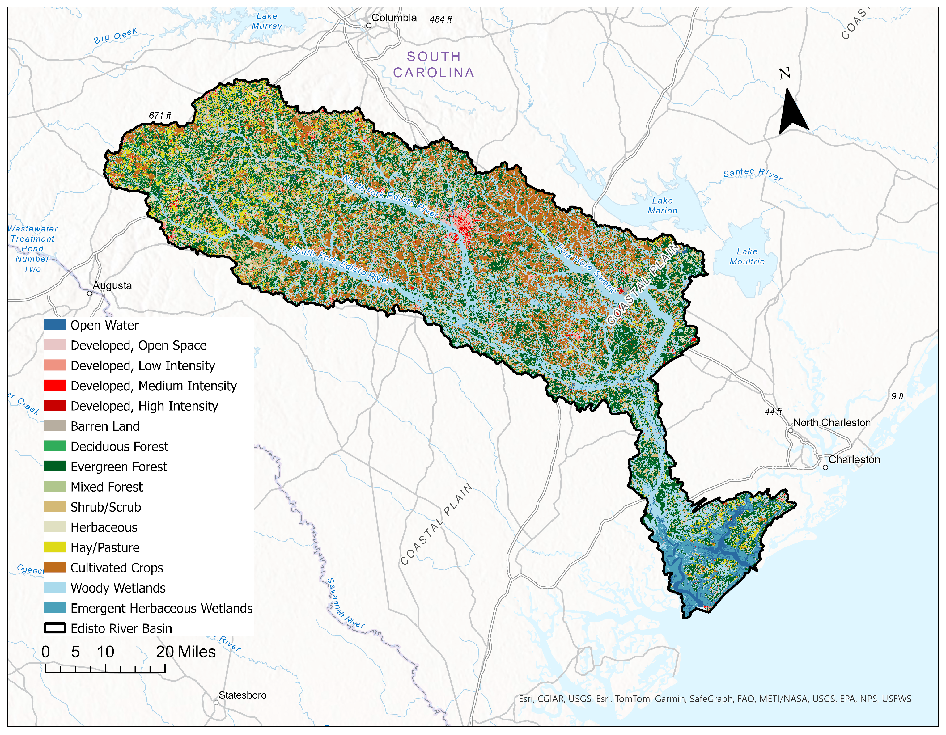
2.1. Study Site

The ERB is in southeastern South Carolina, USA, and encompasses the north and south fork of the Edisto River as it flows out to the Atlantic Ocean (Figure 1). In the northwest part of the basin, the land use is dominated by agriculture, mostly row crops and some timber production. In the southeastern part of the basin, the land use is dominated by timber production. Small communities and one small city, Orangeburg, SC, are scattered throughout the ERB.
The ERB contains one of the longest free-flowing blackwater river systems in the United States [28]. The ERB is approximately 3120 square miles and encompasses about 10% of the state’s land area [29]. Also, ERB is the only river system in South Carolina that is fully within the state [28,30,31]. Its 13 sub-watersheds [32] provide significant ES, including provisioning services (e.g., timber and water supply), regulating services (e.g., flood control, soil management, carbon sequestration), supporting services (e.g., nutrient cycling and soil formation), and cultural services (e.g., recreation use and indigenous knowledge) [19,33]. As one of the largest blackwater riverine systems in the United States, the Edisto River within the ERB boasts a substantial area of bottomland hardwood forests that often sequester a significant amount of carbon per unit area, providing benefits for climate change mitigation [34,35,36,37]. Because of many of these ES benefits, the ERB has over 46,000 acres of privately protected land in the form of conservation easements.
The ERB also provides significant ES in the form of water yield and sediment retention. The Edisto River and surrounding wetlands provide a buffer for flooding events and provide water to an estimated 770,000 people [38]. Because of the buffer that exists around the waterway, the ecosystem is rich in biodiversity and, subsequently, ES. Furthermore, sediment retention reduces eutrophication and organic matter loss, which is detrimental to water quality downstream and reduces the nutrient loss on the landscape [39]. The Edisto River is an area of rich biodiversity and ecosystem services. At over 400 total river miles throughout the whole system, this ecosystem is home to 16 freshwater fish and 13 mussel species that are of conservation concern, along with two fish species on the federally endangered list [28].
While the ERB is rich in biodiversity and other ecosystem services, these ES are declining as resources are continually developed for human consumption. Land use change is significantly affecting this region; development and fragmented forest lands are contributing to the loss of ecosystem services [30,31]. Specific to the ERB, increased water removal from the system and the increased input of pollutants from surrounding agriculture and industrial systems have detrimental effects on ecosystem biodiversity [28,30,40]. Over the last 30 years, increasing population and urbanization have driven the expansion and sprawl of cities [31]. Urban sprawl and the removal of wetlands and forests can have a negative impact on ES [41,42].

2.2. Study Objectives
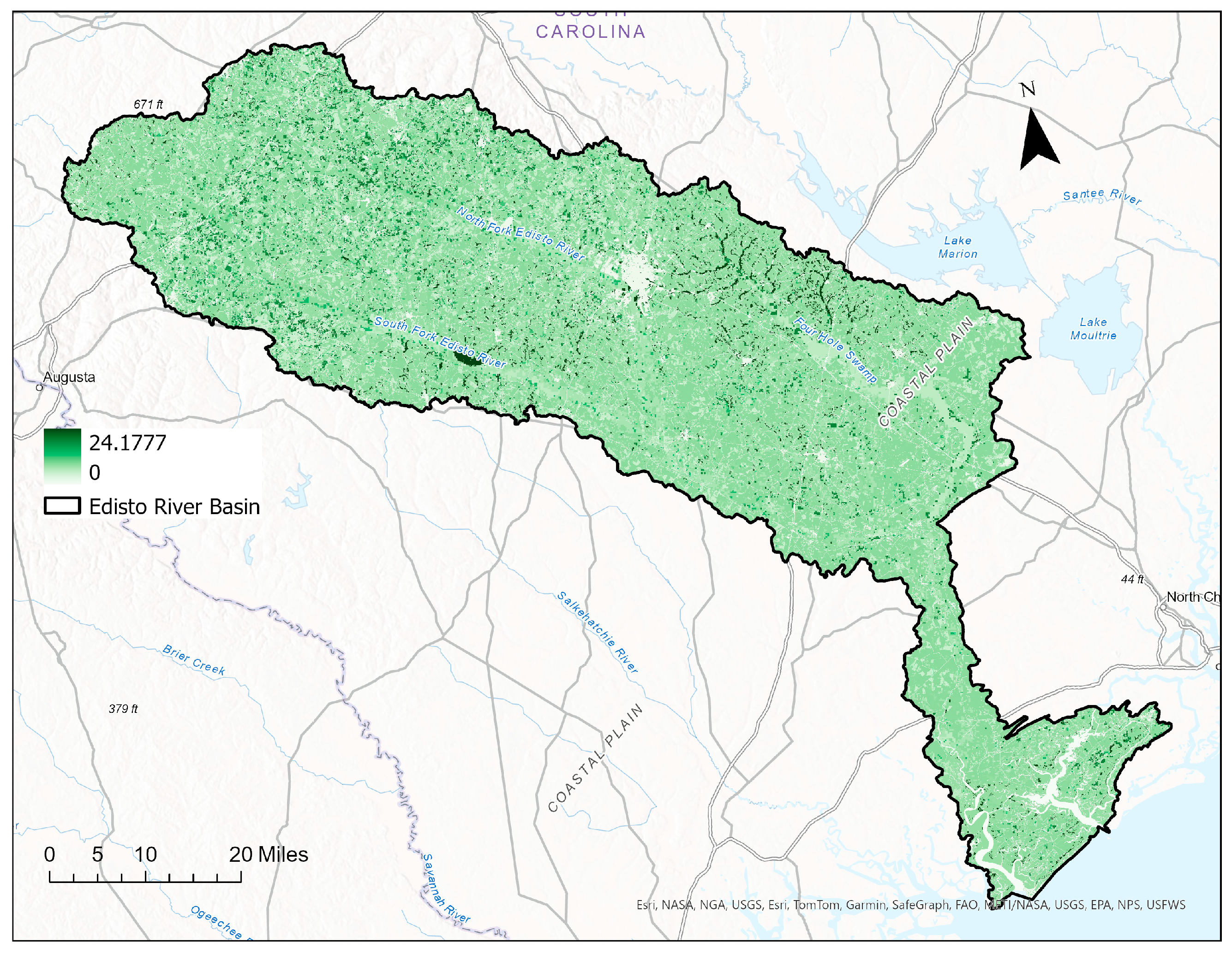
To quantify the ES in the ERB, we utilized the InVEST model to quantify three major ecosystem services: water yield, sediment retention, and carbon stocks [43]. InVEST utilizes a variety of ecological function data to calculate a supply of ES in certain locations. The ecological functions are applied in each pixel of a raster dataset, which allows us to estimate the supply of ES across the landscape of interest [44]. This study used ecological boundaries—watershed—rather than political boundaries to analyze and quantify the ES within the ERB. The sediment delivery ratio and water yield modeling methodology are based on the methodology outlined in Ureta et al. [15], where ES was quantified in the Santee River Basin Network of South Carolina. Using 2021 datasets, we quantified the ES of the ERB using the InVEST modeling. The year 2021 data was used in InVEST modeling to ensure high-quality data, the most recent National Land Cover Database (NLCD), and to create a case for replication in the future for other regions [22,45]. We chose these three ecosystem services, carbon, water yield, and sediment export, due to their importance for localized primary productivity and carbon sequestration. Sediment retention can have a significant impact on soil carbon, nutrient loading, and local biodiversity, and water yield is important as weather patterns shift due to climate change and droughts become more prevalent [46]. Increases in water yield in this context are considered negative benefits because that water runs off and is ultimately lost downstream and is not retained in the ecosystem for use. Next, we explain how water yield, sediment retention, and carbon stocks were modeled in this study.

2.3. Carbon Model

The carbon (C) model was derived from both InVEST modeling capabilities and a method that we developed previously [47] to better quantify carbon across the landscape with available data. This method involves utilizing the forest type dataset from the USDA Forest Service in conjunction with the NLCD to quantify forest carbon stocks more accurately by forest type. Forest Inventory Analysis (FIA) (USDA Forest Service) carbon datasets, which are separated by forest types, were applied to the updated land use maps. The forest-type map with FIA carbon data was then constrained by the NLCD layer so that the forest-type map only covers the updated NLCD forested areas (deciduous, evergreen, or mixed). The final outputs of the model produced carbon stock maps that can be manipulated to measure sequestration and change over time based on both extrapolated carbon data through FIA and land use change. These maps include aboveground and belowground C.
This type of analysis considers one of two major factors that affect carbon sequestration. Tree species and diameter at breast height (DBH) are two major inputs into allometric equations for biomass and, subsequently, carbon sequestration determinations [48]. Previous analyses were limited to carbon sequestration determinations based only on evergreen or hardwood forest types [45]. This study allows for forest type to be resolved spatially, and subsequently, the carbon stock values are more indicative of carbon stocking by forest type, providing a more accurate analysis.
While all of the datasets were manipulated to the specifications required by the InVEST user guide [43], we adjusted the NLCD dataset to add forest type in order to more accurately account for certain land uses and carbon, water yield, and sediment retention capabilities. Previously, when layered in ArcGIS Pro, the NLCD dataset identified only three broad forest types (Evergreen, Hardwoods, and Mixed Forest) which were layered into this dataset.

2.4. Water Yield Model

The water yield (WY) model provides an estimate of the water provisioning from different parts of the landscape by analyzing the precipitation and evapotranspiration of each pixel [44]. The model aims to balance all water movement, which eventually ends up in streams and rivers, assuming that all water will move through the watershed except for water lost due to evapotranspiration. The model analyzes the amount of water that is being released considering the existing land cover and precipitation that is overlaid within a specific pixel (Equation (1)). The WY model provides information about the movement of water across the landscape based on landscape and land cover characteristics.
Y x = 1 A E T x P x × P x
where:
  • Y x = Annual water yield for pixel x
  • A E T x = Annual actual evapotranspiration for pixel x
  • P x = Annual precipitation on pixel x

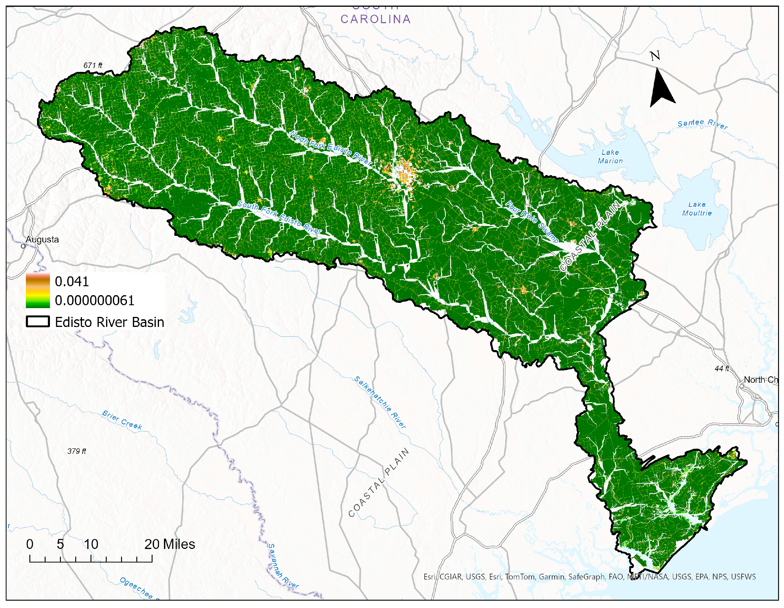
2.5. Sediment Delivery Ratio Model

The Sediment Delivery Ratio (SDR) model quantifies how much sediment is removed from an area of the landscape and will be transported towards the rivers or streams. This is conducted by applying the Revised Universal Soil Loss Equation (RUSLE) to calculate the amount of soil loss per pixel considering the different characteristics of the soil within that pixel (USLEi). The USLEi is comprised of a variety of factors, including rainfall erosivity (Ri), soil erodibility (Ki), slope length-gradient factor (LSi), crop-management factor (Ci), and support practice factor (Pi) [15,44]. The InVEST SDR model utilizes a connectivity index that considers both upslope and downslope factors to determine the net impact of each pixel on sediment delivery throughout the watershed [15]. Once the connectivity index is calculated, the SDRi is computed based on a digital elevation model (DEM) and the biophysical parameters of each landcover type to estimate the number of sediments that are exported by the pixel with and without the existing land cover (Equation (2)). The difference between the sediments exported with and without the existing land cover is considered to be the amount of sediment that is retained by the associated land cover within the pixel.
E i = u s l e i × S D R i
where:
  • E i = Sediment export (ton ha−1 yr−1) from pixel i
  • uslei = universal soil loss equation for pixel i
  • SDRi = Sediment delivery ratio for pixel i
All data sources used are shown in Table 1. The precipitation raster was created from average precipitation data over 30 years [49]. R-factor and evapotranspiration maps were derived from existing data, including precipitation. All raster data was at 30 m × 30 m resolution, and the Albers Equal Area Conic projection was used for spatial alignment in ArcGIS Pro. The InVEST model described the correct processing procedures and would not accept the data if the resolution was not the same for all layers. Upon completion of the model, a .tif file was produced of each ES and its spatial provisioning.

2.6. Validation

Validation is important when considering the ability to value the ecosystem service of interest [44]. The Water Yield (WY) and Sediment Delivery Ratio (SDR) models are validated through time series measurements. For the WY model, stream flow measurements from a study by Beasley et al. (1996) in the Edisto Basin were used for validation [59]. Also, time series measurements of total suspended solids or turbidity were used as an input for the SDR, and the models used were calibrated from observed surveys [46,60].

2.7. Forest Landscape Integrity Index

The Forest Landscape Integrity Index (FLII) was developed by Grantham et al. [58] to show the impact of connectivity on forest and ecosystem health. This metric indicates that both observed and inferred human pressure decreases the health of the ecosystem. Three factors were considered to develop this model. The observed human pressure was derived from a weighted sum of infrastructure and agriculture land use changes. Secondly, inferred human pressures attempt to account for future pressure and consider the distance from pixels with greater observed human pressure. Lastly, loss of forest connectivity was modeled to show forest extent based on forested pixels over time. The data was normalized and added together and is shown as pixels ranging from 1 to 10. The lowest values indicate low quality, while 10 would indicate the highest quality forestland [61]. Much of the US southern forests are classified as low to medium integrity due to fragmentation, the potential for increased parcelization, urban development, and the increase in the population [62]. The FLII was used to identify the most vulnerable areas that would benefit from protection in the form of a carbon project that maximizes ecosystem services.

2.8. Spatial Optimization for Ecosystem Services

The final optimization output relies on developing a standard of additionality for all three studied ecosystem services (e.g., WY, SDR, and carbon storage) after carbon additionality is met. We call the final output of this two-step additionality method ‘total additionality’ (TA). TA includes carbon additionality—the three-pronged test landowners must pass to enter into a carbon project—as a first step (baseline) and co-benefit additionality—the outcome of quantifying ecosystem services via InVEST. The final optimization model (TA) provides an add on to the standard method of additionality, providing a stronger quality assurance claim.
The common practice component of TA requires carbon projects to contribute to a greater carbon sequestration potential of a landscape compared to regional management trends. To quantify the co-benefits of a carbon project utilizing ES modeling, the spatial optimization tool uses different ES spatial outputs to identify areas where these services could be increased. To contribute to additionality feasibility in carbon market protocols, the assumption in the ERB is that the mean values of ES on forested lands are “common practice” and increasing these ecosystem services would contribute to additionality. The FIA data shown in the carbon model herein provides a baseline assessment for determining local forest types and carbon stocks, part one of the TA model.
To create the spatially optimized model, we overlaid all the InVEST outputs for each ES and the Forest Integrity index. To determine if a pixel could be additional, we created a framework specific to the ERB that would consider which pixels would show improvement in ES provisioning (Table 2). Importantly, if this model was used outside of the ERB, these values would be adjusted according to the local ES values and standards for best management practices. Finally, we overlaid each of these filtered layers to create a spatially optimized model where these pixels were aggregated by parcel to show the scale of impact that changes to ES provisioning could have [63] and where already protected areas occur [64].

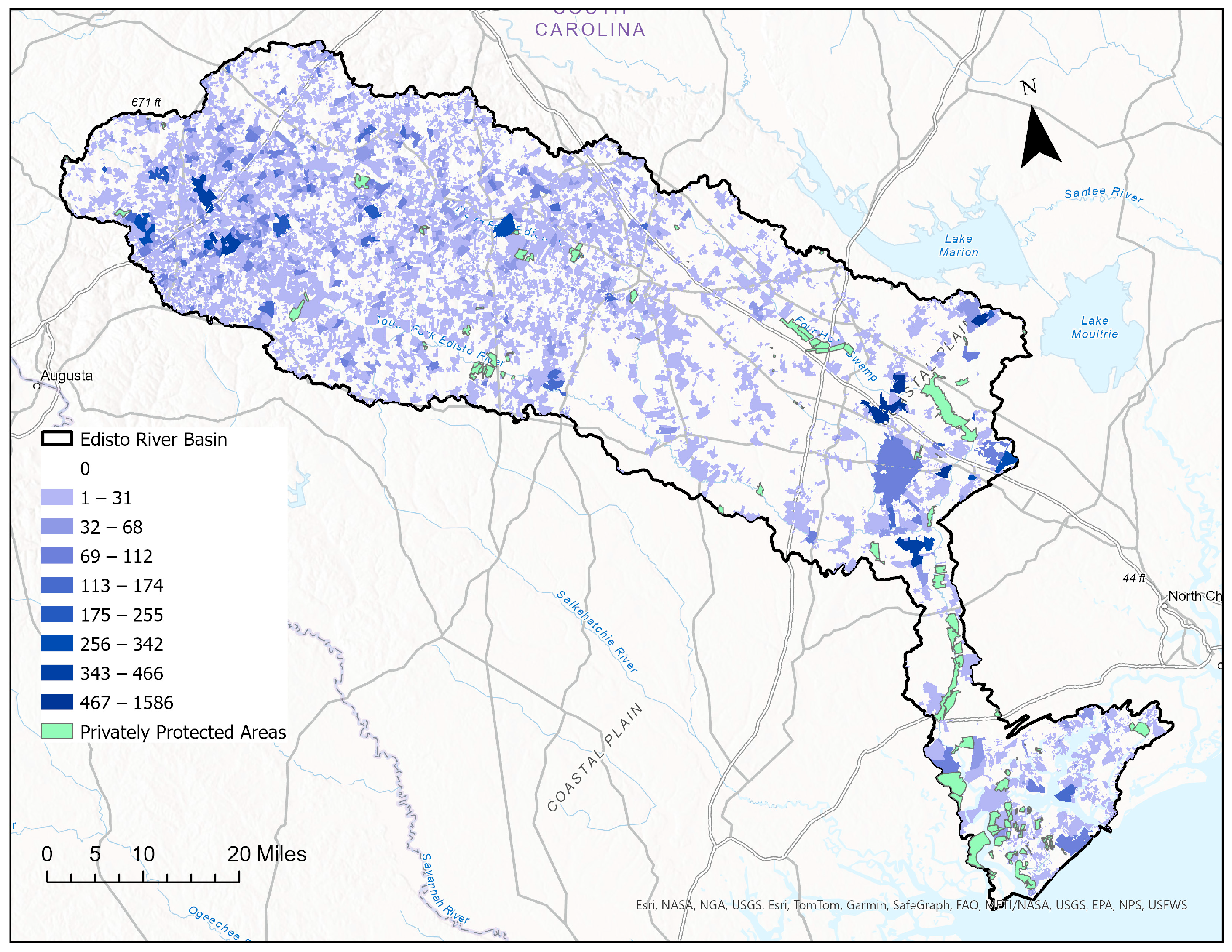
2.9. Additionality Framework for the ERB

When sediment export is already low, there is little change that can be implemented that would be different from business as usual. Because of this, low export values are considered areas with no additionality. Therefore, values greater than the mean show room for improvement and are considered additional in the TA model. Similarly, as water yield increases, ecosystem services due to water retention decrease, but additionality increases, and values greater than the mean are considered as additional in the TA model. Since this model does not account for reforestation or afforestation carbon projects, carbon stocks in the model should be greater than the mean of carbon in developed areas (soil carbon) to show where improved forest management projects are viable. Furthermore, we included the forest integrity index to identify low-quality forests and label them as areas for additionality in the TA model.
The model factors column shows the parameters selected in the model, i.e., a deviation from the mean that will allow for an increase in ecosystem services. This model simply provides a framework for utilizing an ES within additionality assessments. The sediment export variable was determined to be a 20% increase in sediment retention from the mean across the region. The Chesapeake Bay watershed metrics for an increase in sediment retention also use 20% as their metric for success [65]. The water yield variable was derived as the average water yield across forest lands only. The forest integrity variable was defined as all values less than 6: low and medium integrity forestland.

3. Results

ES Quantification

Utilizing InVEST, we quantified three major ecosystem services (Sediment retention, carbon stocks, and water yield) based on 2021 data for the Edisto River Basin. The carbon model (Figure 2) shows how carbon stocks vary significantly among land cover types. We included belowground and aboveground carbon data as derived through on-the-ground measurements [53]. Evergreen C stocks account for 26% of the total stock, while bottomland hardwoods C is 25% of the total stock. Greater levels of C storage were found in bottomland hardwood forests where soil and aboveground stocks were greater. The granular variation in C stocks across the landscape is often due to this contrast, where agriculture is adjacent to bottomland hardwood ecosystems along water bodies. The mean C stock across the basin was 5.65 tons/pixel. Darker green areas indicate greater carbon stocks and light green areas indicate lower stocks. All pixels are 30 × 30 m, 900 m2.
The annual water yield estimates the relative contributions of water from different parts of the landscape (Figure 3) [44]. In this map, the green areas are areas of less water yield, which is a positive ecosystem service. The mean water yield for the basin was 570 ± 271 mm/pixel. This model effectively shows the impact of impervious surfaces on water yield. Separated by land use type, natural land uses (i.e., forested and agriculture) had a mean value of 498 ± 179 mm/pixel. Developed land uses have a mean value of 1237 ± 26 mm/pixel. Light yellow and brown areas indicate the areas of highest runoff, many of these being urban areas, where the assumption is that 100% of rainfall is runoff due to built infrastructure.
Sediment export is similar to water yield since higher sediment export is a negative ecosystem service and indicates increased losses of topsoil and, ultimately, nutrients in that soil. Figure 4 shows the sediment export map for each pixel across the basin. Green pixels are areas of very little sediment export, indicating a high level of soil retention and, ultimately, nutrient retention. Areas of yellow and brown have higher levels of sediment export and could potentially use remedial work.
Figure 5 shows the results of the spatially optimized model; these are the areas where landowners can increase the provision of ecosystem services through new management practices. Water yield and sediment retention were separated to show how different ecosystem services constrain the optimization model. This model only applies to forestland areas that are potentially eligible for carbon financing.
To create the final TA model, these single ES additionality models (Figure 5) were overlaid to create spatial optimization for all ecosystem services (Figure 6). To account for political and ownership boundaries, the TA pixels were then aggregated by parcel throughout the basin, and the number of pixels per parcel is shown (Figure 6). Parcels with a greater number of pixels indicate potentially greater additionality for ecosystem services.
Following the two-step additionality method presented herein, the final number of acres of spatially optimized model for measuring additionality in ecosystem service due to abiding by carbon market requirements is 23,709 acres. This spatial layer shows areas that could provide additional ES benefits if best management practices are introduced. Because the model considers additionality, these are the areas that could provide the most financial benefit to landowners through ES improvement. While disaggregated, these areas are on existing forestland where improved forest management projects could be implemented. We also added privately protected areas to the map to show areas that are already under conservation easement. In Table 3, Parcel Total Area shows the total acres of parcels that have TA model pixels fall within the area that could be affected by improved conservation finance. The Modeled TA total area shows how many acres by individual pixel are modeled to have an additional increase in ES provisioning. We also included only pixels that fall within parcels greater than 20 acres separately, as these parcels are more likely to be accessible for forestry and enrolled in carbon programs.

4. Discussion

In this study, we attempt to quantify the ecosystem services of the ERB based on 2021 land use/land cover data utilizing the InVEST software. These individual ES models provide a baseline for each ES to spatially optimize conservation. The ERB is a valuable case study because 52% of the land is classified as forest, providing many ecosystem services, including carbon sequestration, and representative of the southern coastal plain ecosystem. Total carbon stocks across the ERB basin are similar compared to many locations in the southeast that have multiple land uses, including agriculture and bottomland hardwood forests [53]. Due to substantial forestry operations, these forests are often well stocked, and contribute to natural climate solutions. On the contrary, the Forest Landscape Integrity mapping indicates that much of this land is of low quality due to human intervention, and various management practices are needed to increase ecosystem services provisioning [58,62], and our baseline mapping agrees with this assessment [58]. Based on the results in Figure 4, sediment export is minimal across the basin, presumably due to significant forested areas and well-implemented best management practices that protect water quality in forestry operations [66]. Water yield is also visually correlated to the land cover, where urban and agriculture systems have more runoff than forested ecosystems that trap water.

4.1. Land Use and Conservation

Land use is changing rapidly as populations increase and as wood products markets shift. The National Land Cover Database from USGS indicates that urbanization is increasing throughout South Carolina [45]. Many areas once considered rural in South Carolina are being developed as land prices are low relative to other areas of the country, and as the population of South Carolina increases, the risk of conversion is increasing [67,68,69]. Quantifying the baseline of ecosystem services indicates the need to increase protection and conservation. Traditional methods for protection include conservation easements, deeding land to public entities, or reducing agriculture and timber harvesting. Conservation easements limit land conversion to residential or commercial property while still allowing for farming or timber production in most cases [70]. These easements can be a good choice for landowners due to their ability to allow for continued management of natural resources while also receiving tax credits and guidance from local land trusts. Easements can be a good first step for conservation as they reduce land use change, but continued management using conservation practices is necessary to increase ecosystem service provisioning. Conservation management at the landowner level may yield small changes that would impact ecosystem services at a stand, farm, or property level, such as improved forest management to increase carbon at the plot level or utilizing best management practices to reduce water runoff. As market-based financing mechanisms for conserving land that values carbon and other ecosystem services become more ubiquitous, the need for a single metric of quantification can aid in comparing the outcomes of these conservation mechanisms. While these management tactics provide minimal increases in ecosystem services, the value of market-based financing mechanisms is in reducing land conversion to developed areas.

4.2. Increasing Impact through More Rigorous Additionality

Market-based solutions that are driven by corporate conservation financing often rely on multiple additionality principles to ensure that the practices change or carbon sequestration that they are using to offset their emissions would not have occurred without the financing [71]. In many cases, it can be difficult to identify true additionality; historical and modeled management practices inform what may happen in the future but may not actually reflect what will happen. To aid in developing a more rigorous common practice baseline, the TA model developed in this study identifies areas of land that would most benefit from enhancing forest management (Figure 6) and best management practices to increase co-benefits. While it is important to decrease atmospheric carbon through nature-based solutions, a more holistic approach to managing forest land is to consider other ecosystem services and the co-benefits provided [17]. Furthermore, recent market data shows that carbon projects with co-benefits have a price premium in the voluntary market, where carbon credits with co-benefits were averaging $10.08 a credit and credits without co-benefits were averaging $6.07 [8]. Currently, methods for quantifying carbon project co-benefits include using the Climate, Communities, and Biodiversity Standard from Verra [72] or quantifying how certain United Nations Sustainable Development Goals (SDGs) [73] are maximized. In the future, these types of ES models could provide the necessary quantification to increase the value of the credits in the VCM [10,74]. The model shows areas that could use conservation management to reach or exceed the mean ES values for the basin. Furthermore, this model is a framework that could allow for additional justification for establishing carbon projects in areas where a carbon project’s co-benefits could be optimized. If these models are to be used in mainstream carbon and biodiversity projects, better data resolution and more recent data are needed to account for ES accurately.

4.3. Spatial Model for Additionality

The optimized model shows relatively fragmented areas for additional ecosystem services. In practice, carbon projects would include more contiguous property, covering more land area. The spatially optimized areas are largely not contiguous, and carbon projects typically will go beyond the confines of the TA model and include larger, contiguous land areas. To account for this, the parcel map was overlaid with the TA pixels, and parcels with a greater number of pixels would have a greater justification for increased ES provisioning. Considering practical implementation on the ground, it is important to include the costs of compliance within these carbon protocols; landowners typically need large land holdings to achieve a return on investment. Innovative protocols that include the aggregation of multiple landowners and land areas into one project could provide a pathway to enrollment for smaller landowners, along with quantifying ES to increase prices. Carbon projects using this framework would also help increase ES provisioning across the parcel, thus increasing ES even more than quantified herein. As indicated through the forest integrity layer, these pixels exist in degraded forests, i.e., limited management or connectivity. Furthermore, the model also shows that many of the areas that are selected are near farmland or other land use types. It is important to show that there is potential for increasing ecosystem services, including carbon sequestration, through management. Research and protocol development that would enhance ecosystem services and carbon projects on smaller plots and properties would be beneficial to both additional carbon sequestration and conserving ES in previously difficult-to-manage areas [75].

5. Conclusions

Conservation of lands in ERB is important, and ES quantification and valuation could help identify the priority areas for conservation. As co-benefits become more valuable in the market, this is an opportunity to use an existing environmental market to achieve multiple land use benefits in addition to carbon sequestration [74]. InVEST modeling can provide the initial framework for modeling ES provisioning and spatial optimization of ES. As more data is collected, TA models can be updated to show positive changes in ecosystem function, where these ecosystems are not only sequestrating more carbon but also providing more co-benefits in terms of water and sediment retention. Considering the impact of land use change on these ES, along with other tradeoffs, including timber production, hunting, and recreational uses, is crucial to effectively manage the ERB. This study indicates that via our standards of ES additionality, there are a significant number of tracts within the ERB that would achieve additionality if best management practices through carbon projects or other projects were implemented. Scaling this study to other regions would provide a necessary method to quantify ES in a way that will allow them to be optimized and conserved. The spatial optimization of ES enhancement will allow market-based solutions to select areas that need the most additional management and help achieve true additionality and climate benefits. Land use change is increasing, and ES are being threatened. As data quality increases, models provided herein will be paramount in quantifying ES and in justifying funding to landowners who implement conservation management and aid in mitigating land use change.

Author Contributions

Conceptualization, L.C. and M.M.; methodology, L.C. and M.M.; validation, M.M.; formal analysis, L.C.; data curation, L.C.; writing—original draft preparation, L.C.; writing—review and editing, M.M. and T.L.O.; visualization, L.C.; supervision, T.L.O.; project administration, M.M. and T.L.O.; funding acquisition, T.L.O., M.M. and L.C. All authors have read and agreed to the published version of the manuscript.

Funding

This research was partially funded by the South Carolina Water Resources Center at Clemson University and the U.S. Geological Survey. The APC was funded by the Clemson University Libraries Open Access Publishing Fund.

Data Availability Statement

All data sources for the InVEST model are included in the article. For specific outputs and data requests, please contact the corresponding author.

Conflicts of Interest

The authors declare no conflicts of interest.

References

  1. Zickfeld, K.; MacIsaac, A.J.; Canadell, J.G.; Fuss, S.; Jackson, R.B.; Jones, C.D.; Lohila, A.; Matthews, H.D.; Peters, G.P.; Rogelj, J.; et al. Net-Zero Approaches Must Consider Earth System Impacts to Achieve Climate Goals. Nat. Clim. Chang. 2023, 13, 1298–1305. [Google Scholar] [CrossRef]
  2. Rogelj, J.; Schaeffer, M.; Meinshausen, M.; Knutti, R.; Alcamo, J.; Riahi, K.; Hare, W. Zero Emission Targets as Long-Term Global Goals for Climate Protection. Environ. Res. Lett. 2015, 10, 105007. [Google Scholar] [CrossRef]
  3. Galatowitsch, S.M. Carbon Offsets as Ecological Restorations. Restor. Ecol. 2009, 17, 563–570. [Google Scholar] [CrossRef]
  4. Soto, J.R.; Adams, D.C.; Escobedo, F.J. Landowner Attitudes and Willingness to Accept Compensation from Forest Carbon Offsets: Application of Best-Worst Choice Modeling in Florida USA. Policy Econ. 2016, 63, 35–42. [Google Scholar] [CrossRef]
  5. Streck, C. How Voluntary Carbon Markets Can Drive Climate Ambition. J. Energy Nat. Resour. Law. 2021, 39, 367–374. [Google Scholar] [CrossRef]
  6. Tahvonen, O.; Rautiainen, A. Economics of Forest Carbon Storage and the Additionality Principle. Resour. Energy Econ. 2017, 50, 124–134. [Google Scholar] [CrossRef]
  7. Ruseva, T.; Marland, E.; Szymanski, C.; Hoyle, J.; Marland, G.; Kowalczyk, T. Additionality and Permanence Standards in California’s Forest Offset Protocol: A Review of Project and Program Level Implications. J. Environ. Manag. 2017, 198, 277–288. [Google Scholar] [CrossRef]
  8. Donofrio, S.; Maguire, P.; Daley, C.; Calderon, C.; Lin, K. The Art of Integrity: State of the Voluntary Carbon Markets 2022 Q3; Ecosystem Marketplace: Washington, DC, USA, 2022. [Google Scholar]
  9. COP26: Voluntary Carbon Market Value Tops $1 Bil in 2021. Available online: https://www.spglobal.com/commodityinsights/en/market-insights/podcasts/energy-evolution/040723-ceraweek-powerflex-electric-vehicle-gridpoint-energy-management-transition (accessed on 11 April 2023).
  10. Phelps, J.; Webb, E.L.; Adams, W.M. Biodiversity Co-Benefits of Policies to Reduce Forest-Carbon Emissions. Nat. Publ. Group. 2012, 2, 497–503. [Google Scholar] [CrossRef]
  11. West, T.A.P.; Börner, J.; Sills, E.O.; Kontoleon, A. Overstated Carbon Emission Reductions from Voluntary REDD + Projects in the Brazilian Amazon. Proc. Natl. Acad. Sci. USA 2020, 117, 24188–24194. [Google Scholar] [CrossRef]
  12. Badgley, G.; Freeman, J.; Hamman, J.J.; Haya, B.; Trugman, A.T.; Anderegg, W.R.L.; Cullenward, D. Systematic Over-Crediting in California’s Forest Carbon Offsets Program. bioRxiv 2021, 28, 1433–1445. [Google Scholar] [CrossRef]
  13. Remucal, J.M.; Mcgee, J.D.; Fehrenbacher, M.M.; Best, C.; Mitchell, R.J. Application of the Climate Action Reserve’s Forest Project Protocol to a Longleaf Pine Forest under Restoration Management. J. For. 2013, 111, 59–66. [Google Scholar] [CrossRef]
  14. Puhlick, J.J.; Brantley, S.T.; O’Halloran, T.L.; Clay, L.; Klepzig, K.D. Perspectives: Carbon Markets Might Incentivize Poorer Ecological Outcomes in Longleaf Pine Ecosystems. For. Ecol. Manag. 2022, 520, 120421. [Google Scholar] [CrossRef]
  15. Ureta, J.C.; Clay, L.; Motallebi, M.; Ureta, J. Quantifying the Landscape ’ s Ecological Benefits—An Analysis of the Effect of Land Cover Change on Ecosystem Services. Land 2020, 10, 21. [Google Scholar] [CrossRef]
  16. Schägner, J.P.; Brander, L.; Maes, J.; Hartje, V. Mapping Ecosystem Services’ Values: Current Practice and Future Prospects. Ecosyst. Serv. 2013, 4, 33–46. [Google Scholar] [CrossRef]
  17. Schröter, M.; Remme, R.P. Spatial Prioritisation for Conserving Ecosystem Services: Comparing Hotspots with Heuristic Optimisation. Landsc. Ecol. 2016, 31, 431–450. [Google Scholar] [CrossRef]
  18. Li, J.; Xie, B.; Dong, H.; Zhou, K.; Zhang, X. The Impact of Urbanization on Ecosystem Services: Both Time and Space Are Important to Identify Driving Forces. J. Environ. Manag. 2023, 347, 119161. [Google Scholar] [CrossRef]
  19. Mori, A.S.; Lertzman, K.P.; Gustafsson, L. Biodiversity and Ecosystem Services in Forest Ecosystems: A Research Agenda for Applied Forest Ecology. J. Appl. Ecol. 2017, 54, 12–27. [Google Scholar] [CrossRef]
  20. Millenium Ecosystem Assessment. Ecosystems and Human Well-Being: Synthesis; Island Press: Washington, DC, USA, 2005. [Google Scholar]
  21. Dertien, J.S.; Baldwin, R.F. Does Scale or Method Matter for Conservation? Application of Directional and Omnidirectional Connectivity Models in Spatial Prioritizations. Front. Conserv. Sci. 2023, 4, 976914. [Google Scholar] [CrossRef]
  22. Kang, M.J.; Siry, J.P.; Colson, G.; Ferreira, S. Do Forest Property Characteristics Reveal Landowners’ Willingness to Accept Payments for Ecosystem Services Contracts in Southeast Georgia, U.S.? Ecol. Econ. 2019, 161, 144–152. [Google Scholar] [CrossRef]
  23. Michaelowa, A.; Shishlov, I.; Brescia, D.; Michaelowa, A. Evolution of International Carbon Markets: Lessons for the Paris Agreement Article Title: Evolution of International Carbon Markets-Lessons for the Paris Agreement. Wiley Clim. Chang. 2019, 10, e613. [Google Scholar] [CrossRef]
  24. Cooper, L.; MacFarlane, D. Climate-Smart Forestry: Promise and Risks for Forests, Society, and Climate. PLoS Clim. 2023, 2, e0000212. [Google Scholar] [CrossRef]
  25. The World Bank. State and Trends of Carbon Pricing 2024; The World Bank: Washington, DC, USA, 2024. [Google Scholar]
  26. American Carbon Registry. Improved Forest Management Methodology for Quantifying Removals and Emission Reductions through Increased Forest Carbon Sequestration on Non-Federal US Forestlands; American Carbon Registry: North Little Rock, AR, USA, 2018. [Google Scholar]
  27. Galik, C.S.; Murray, B.C.; Mitchell, S.; Cottle, P. Alternative Approaches for Addressing Non-Permanence in Carbon Projects: An Application to Afforestation and Reforestation under the Clean Development Mechanism. Mitig. Adapt. Strat. Glob. Chang. 2016, 21, 101–118. [Google Scholar] [CrossRef]
  28. Berzinis, R.W. Long-Term and Two-Period Analysis of Hydrologic Conditions of the South Edisto River. J. S. Carol. Water Resour. 2017, 4, 13–20. [Google Scholar]
  29. SCDNR. An Overview of the Eight Major River Basins of South Carolina; SCDNR: West Columbia, SC, USA, 2013. [Google Scholar]
  30. Napton, D.E.; Auch, R.F.; Headley, R.; Taylor, J.L. Land Changes and Their Driving Forces in the Southeastern United States. Reg. Environ. Chang. 2010, 10, 37–53. [Google Scholar] [CrossRef]
  31. Venter, O.; Sanderson, E.W.; Magrach, A.; Allan, J.R.; Beher, J.; Jones, K.R.; Possingham, H.P.; Laurance, W.F.; Wood, P.; Fekete, B.M.; et al. Sixteen Years of Change in the Global Terrestrial Human Footprint and Implications for Biodiversity Conservation. Nat. Commun. 2016, 7, 12558. [Google Scholar] [CrossRef]
  32. DHEC. Watershed Water Quality Assessment Edisto River Basin 2012; DHEC: Colombia, SC, USA, 2012. [Google Scholar]
  33. de Groot, D.; Brander, L.; Max Finlayson, C. Wetland Ecosystem Services. In The Wetland Book: I: Structure and Function, Management, and Methods; Springer: Dordrecht, The Netherlands, 2018; pp. 323–333. ISBN 9789048196593. [Google Scholar]
  34. Miller, K.A.; Snyder, S.A.; Kilgore, M.A. An Assessment of Forest Landowner Interest in Selling Forest Carbon Credits in the Lake States, USA. For. Policy Econ. 2012, 25, 113–122. [Google Scholar] [CrossRef]
  35. Busch, J.; Godoy, F.; Turner, W.R.; Harvey, C.A. Biodiversity Co-Benefits of Reducing Emissions from Deforestation under Alternative Reference Levels and Levels of Finance. Conserv. Lett. 2011, 4, 101–115. [Google Scholar] [CrossRef]
  36. Gosnell, H.; Charnley, S.; Stanley, P. Climate Change Mitigation as a Co-Benefit of Regenerative Ranching: Insights from Australia and the United States. Interface Focus. 2020, 10, 20200027. [Google Scholar] [CrossRef]
  37. Krauss, K.W.; Noe, G.B.; Duberstein, J.A.; Conner, W.H.; Stagg, C.L.; Cormier, N.; Jones, M.C.; Bernhardt, C.E.; Graeme Lockaby, B.; From, A.S.; et al. The Role of the Upper Tidal Estuary in Wetland Blue Carbon Storage and Flux. Glob. Biogeochem. Cycles 2018, 32, 817–839. [Google Scholar] [CrossRef]
  38. Pattison-Williams, J.K.; Pomeroy, J.W.; Badiou, P.; Gabor, S. Wetlands, Flood Control and Ecosystem Services in the Smith Creek Drainage Basin: A Case Study in Saskatchewan, Canada. Ecol. Econ. 2018, 147, 36–47. [Google Scholar] [CrossRef]
  39. Hamel, P.; Chaplin-Kramer, R.; Sim, S.; Mueller, C. A New Approach to Modeling the Sediment Retention Service (InVEST 3.0): Case Study of the Cape Fear Catchment, North Carolina, USA. Sci. Total Environ. 2015, 524–525, 166–177. [Google Scholar] [CrossRef] [PubMed]
  40. Lendemer, J.C. Bacidia gullahgeechee (Bacidiaceae, Lecanoromycetes) an Unusual New Species Potentially Endemic to the Globally Unique Ashepoo-Combahee-Edisto River Basin of Southeastern North America. Bryologist 2018, 121, 536–546. [Google Scholar] [CrossRef]
  41. Billah, M.M.; Goodall, J.L. Annual and Interannual Variations in Terrestrial Water Storage during and Following a Period of Drought in South Carolina, USA. J. Hydrol. 2011, 409, 472–482. [Google Scholar] [CrossRef]
  42. Moriasi, D.N.; Arnold, J.G.; Liew, M.W.; Van Bingner, R.L.; Harmel, R.D.; Veith, T.L. Model Evaluation Guidelines for Systematic Quantification of Accuracy in Watershed Simulations. Trans. ASABE 1983, 50, 885–900. [Google Scholar] [CrossRef]
  43. InVEST User Guide 3.14. Available online: https://storage.googleapis.com/releases.naturalcapitalproject.org/invest-userguide/latest/index.html (accessed on 9 June 2021).
  44. Nelson, E.; Ennaanay, D.; Wolny, S.; Olwero, N.; Vigerstol, K.; Penning-ton, D.; Mendoza, G.; Aukema, J.; Foster, J.; Forrest, J.; et al. InVEST 3.6.0 User’s Guide. The Natural Capital Project; Stanford University: Stanford, CA, USA, 2018. [Google Scholar]
  45. U.S. Geological Survey. National Land Cover Database; Earth Resources Observation and Science (EROS) Center: Sioux Falls, SD, USA, 2018. [Google Scholar]
  46. McCarney-Castle, K.; Childress, T.M.; Heaton, C.R. Sediment Source Identification and Load Prediction in a Mixed-Use Piedmont Watershed, South Carolina. J. Environ. Manag. 2017, 185, 60–69. [Google Scholar] [CrossRef]
  47. Clay, L.; Motallebi, M.; Song, B. An Analysis of Common Forest Management Practices for Carbon Sequestration in South Carolina. Forests 2019, 10, 949. [Google Scholar] [CrossRef]
  48. Pearson, T.R.H.; Brown, S.L.; Birdsey, R.A. Measurement Guidelines for the Sequestration of Forest Carbon; USDA: Washington, DC, USA, 2007. [Google Scholar]
  49. PRISM Climate Group—Precipitation. Available online: https://prism.oregonstate.edu/recent/ (accessed on 9 June 2021).
  50. South Carolina Dept of Natural Resources. SCDNR—LiDAR Data Status by County. Available online: https://www.dnr.sc.gov/gis/lidar.html (accessed on 2 February 2021).
  51. Renard, K.G.; Freimund, J.R. Using Monthly Precipitation Data to Estimate the R-Factor in the Revised USLE. J. Hydrol. 1994, 157, 287–306. [Google Scholar] [CrossRef]
  52. ESRI USA Soils Erodibility Factor|ArcGIS Hub. Available online: https://hub.arcgis.com/datasets/ac1bc7c30bd4455e85f01fc51055e586/explore (accessed on 3 September 2024).
  53. Alvarez, M. Forest Inventory and Analysis Database 2021; U.S. Department of Agriculture: Washington, DC, USA, 2023. [Google Scholar]
  54. Allen, R.G.; Pereira, L.S.; Raes, D.; Smith, M. FAO Irrigation and Drainage Paper No. 56: Crop Evapotranspiration; FAO—Food and Agriculture Organization of the United Nations: Rome, Italy, 1998. [Google Scholar]
  55. Soil Survey Staff, Natural Resources Conservation Service, United States Department of Agriculture. Web Soil Survey. Available online: http://websoilsurvey.sc.egov.usda.gov/ (accessed on 24 February 2021).
  56. USDA Forest Service—National Forest Type Dataset. Available online: https://data.fs.usda.gov/geodata/rastergateway/forest_type/index.php (accessed on 9 June 2021).
  57. U.S. Geological Survey. The National Hydrography Dataset (NHD) [WWW Document]. 2018. Available online: https://nhd.usgs.gov/ (accessed on 3 May 2021).
  58. Grantham, H.S.; Duncan, A.; Evans, T.D.; Jones, K.R.; Beyer, H.L.; Schuster, R.; Walston, J.; Ray, J.C.; Robinson, J.G.; Callow, M.; et al. Anthropogenic Modification of Forests Means Only 40% of Remaining Forests Have High Ecosystem Integrity. Nat. Commun. 2020, 11, 5978. [Google Scholar] [CrossRef]
  59. Beasley, B.; Marshall, W.; Miglarese, A.; James, S.; Vanden Houten, C.; The Edisto River Basin Project Report. South Carolina Department of Natural Resources. 1996; pp. 1–240. Available online: https://www.dnr.sc.gov/water/river/pdf/1996EdistoProjectReport.pdf (accessed on 9 October 2024).
  60. U.S. Geological Survey. Surface Water Data for USA: USGS Monthly Statistics; U.S. Geological Survey: Reston, VA, USA, 2024. [Google Scholar]
  61. Forest Landscape Integrity Index. Available online: https://www.forestlandscapeintegrity.com/home (accessed on 20 March 2022).
  62. Moldenhauer, M.C.; Bolding, S.M.C. Parcelization of South Carolina’s Private Forestland: Loggers’ Reactions to a Growing Threat. For. Prod. J. 2009, 6, 37–43. [Google Scholar]
  63. Loveland Technologies Regrid Data. Loveland Technol. Available online: https://regrid.com/terms/researchers-academics (accessed on 3 May 2024).
  64. U.S. Geological Survey. Protected Areas Database of the United States (PAD-US) 4.0 [Dataset]; U.S. Geological Survey (USGS) Gap Analysis Project (GAP): Reston, VA, USA, 2024. [Google Scholar]
  65. Zhang, Q.; Blomquist, J.D.; Fanelli, R.M.; Keisman, J.L.D.; Moyer, D.L.; Langland, M.J. Progress in Reducing Nutrient and Sediment Loads to Chesapeake Bay: Three Decades of Monitoring Data and Implications for Restoring Complex Ecosystems. Wiley Interdiscip. Rev. Water 2023, 10, e1671. [Google Scholar] [CrossRef]
  66. Welch, H. Forestry BMPs in South Carolina: Compliance and Implementation Monitoring Report; South Carolina Forestry Commission: Columbia, SC, USA, 2020. [Google Scholar]
  67. Alig, R.; Stewart, S.; Wear, D.; Stein, S. Conversions of Forest Land: Trends, Determinants, Projections, and Policy Considerations. In Proceedings of the Advances in Threat Assessment and Their Application to Forest and Rangeland Management, Boulder, CO, USA, 18–20 July 2006. [Google Scholar]
  68. Nowak, D.J.; Walton, J.T. Projected Urban Growth (2000–2050) and Its Estimated Impact on the US Forest Resource. J. For. 2005, 103, 383–389. [Google Scholar] [CrossRef]
  69. Johnson, K.K.; Parton, L.; Nolte, C.; Williamson, M.; Nogeire-McRae, T.; Paudel, J.; Brandt, J. Moving to the Country: Understanding the Effects of COVID-19 on Property Values and Farmland Development Risk. J. Hous. Econ. 2023, 62, 101955. [Google Scholar] [CrossRef]
  70. Merenlender, A.M.; Huntsinger, L.; Guthey, G.; Fairfax, S.K. Land Trusts and Conservation Easements: Who Is Conserving What for Whom? Patronatos Agrarios y Servicios de Conservación: ¿Quién Está Conservando Qué Para Quién? Conserv. Biol. 2004, 18, 65–76. [Google Scholar] [CrossRef]
  71. Haya, B.K.; Evans, S.; Brown, L.; Bukoski, J.; Butsic, V.; Cabiyo, B.; Jacobson, R.; Kerr, A.; Potts, M.; Sanchez, D.L. Comprehensive Review of Carbon Quantification by Improved Forest Management Offset Protocols. Front. For. Glob. Chang. 2023, 6, 958879. [Google Scholar] [CrossRef]
  72. Climate, Community & Biodiversity Standards—Verra. Available online: https://verra.org/programs/ccbs/ (accessed on 17 July 2024).
  73. Hák, T.; Janoušková, S.; Moldan, B. Sustainable Development Goals: A Need for Relevant Indicators. Ecol. Indic. 2016, 60, 565–573. [Google Scholar] [CrossRef]
  74. Lee, D.-H.; Kim, D.-H.; Kim, S.-I. Characteristics of Forest Carbon Credit Transactions in the Voluntary Carbon Market. Clim. Policy 2018, 18, 235–245. [Google Scholar] [CrossRef]
  75. White, A.E.; Lutz, D.A.; Howarth, R.B.; Soto, J.R. Small-Scale Forestry and Carbon Offset Markets: An Empirical Study of Vermont Current Use Forest Landowner Willingness to Accept Carbon Credit Programs. PLoS ONE 2018, 13, e0201967. [Google Scholar] [CrossRef]
Figure 1. NLCD land use in the ERB, year 2021.
Forests 15 01796 g001
Figure 2. Carbon in tons (t C/pixel, year 2021).
Forests 15 01796 g002
Figure 3. Water yield in mm/pixel for the ERB, the year 2021.
Forests 15 01796 g003
Figure 4. Sediment export in tons/pixel across the ERB in the year 2021.
Forests 15 01796 g004
Figure 5. ES Additionality Model, (a) areas for water yield improvement, and (b) areas for sediment retention improvement. The results are binary, where all colored values (green for water yield improvement and brown for sediment export) are considered pixels that are included in the final TA model because they are additional.
Forests 15 01796 g005
Figure 6. Total Additionality (TA) model for forested areas (pixel count by parcel).
Forests 15 01796 g006
Table 1. Data sources for InVEST model.
DataYearData TypeApplicable ModelSources
Digital Elevation Model2015Raster (.tif)SDR[50]
Iso-erosivity map (R factor)2021Raster (.tif)SDR[51]
Soil erodibility map (K factor)2015Raster (.tif)SDR[52]
Land use/land cover2021Raster (.tif)SDR, WY, C[45,53]
Precipitation1990–2020 averageRaster (.tif)WY[49]
EvapotranspirationFrom precipitation dataRaster (.tif)WY[54]
Depth to root restricting layer2019 dataRaster (.tif)WY[55]
Plant available water fraction2019 dataRaster (.tif)WY[55]
Forest type carbon stocks2021 dataNon-spatial data (.csv)C[53]
Forest type (part of land use land cover raster)2008Raster (.tif)SDR, WY, C[56]
Watershed boundary2013Vector (.shp)SDR, WY[57]
Biophysical tableNANon-spatial data (.csv)SDR, WY, C[53,54,55]
Forest Integrity Index2020Raster (.tif)Scale: 1–10[58]
Table 2. Statistical output from InVEST model and spatial optimization factors for the Edisto River Basin.
MinimumMaximumMeanSt. DevVariables Used in TA Model
Sediment Export (tons/pixel)0305.790.0250.50>0.0068
Water Yield (mm/pixel)181.861308.16570.19270.99>412.95
Forest Integrity Index (scale)0101.5661.861<6
Table 3. Land area for implementing TA model.
Parcel Total AreaModeled TA Total Area
All Parcels719,018 acres23,709 acres
Parcels greater than 20 acres70,509 acres3763 acres
Disclaimer/Publisher’s Note: The statements, opinions and data contained in all publications are solely those of the individual author(s) and contributor(s) and not of MDPI and/or the editor(s). MDPI and/or the editor(s) disclaim responsibility for any injury to people or property resulting from any ideas, methods, instructions or products referred to in the content.

