Abstract
Demand for high-quality white oak sawlogs in Kentucky has been increasing for decades. Concurrently, Kentucky is witnessing ecological shifts in the historically white oak-dominated forests, mirroring the structural changes in oak forests in the eastern US. This demand–supply dissonance presents a growing concern among stakeholders on the sustainability of white oak and its associated economic implications. In this context, the objective of this study was to assess the potential economic impacts of the projected white oak timber supply following an overall increased supply of white oak sawlogs but reduced supply of high-quality white oak sawlogs in Kentucky. Results generated from a dynamic computable general equilibrium (CGE) model indicate a cumulative present-value GDP reduction of USD 3.66 billion, a USD 0.71 billion decline in consumer welfare, and other sectoral contractions over 40 years (2018–2058). These results can be used to advocate for more proactive forest management practices to stabilize a sustained supply of high-quality white oak timber in Kentucky and beyond.
1. Introduction
White oak (Quercus alba L.) is a commercially important timber resource in the Commonwealth of Kentucky. Nearly 11% of growing stock volume in the Commonwealth comprises white oak, and about 42% of Kentucky’s timberland area is under white oak-dominated forests [1]. In 2018, roughly 13% of all roundwood harvested in the state was select white oak [2]. Therefore, the sustainable management of highly valued white oak forests is a desirable goal in Kentucky.
The sustainable supply of white oak timber is critical to white oak-dependent industries, especially wood products manufacturing and distilleries sectors: two of the largest sectors that use white oak logs in their production process. The primary and secondary wood manufacturing sectors use white oak logs for lumber, railway ties, pallets, wood containers, and other wood products; the distilling industries use barrels primarily made from high-quality white oak stave logs for aging the bourbons (Figure 1). While the federal law mandates that American bourbon be made in charred new oak containers [3], it is the peculiar structural features of white oak, i.e., the presence of medullary rays and tyloses, that renders its woods impervious, thus making them ideal for tight cooperage [4]. Kentucky white oak lumber and forest products generate around USD 61 million in annual revenue, while the barrel stave production contributes about USD 134 million in annual revenue [5]. Additionally, Kentucky’s distilling industry generated around 20,100 jobs, with an annual payroll of USD 1 billion, producing USD 8.6 billion of total economic output in 2018 [6].
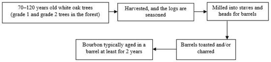
Figure 1.
A typical supply chain from stump to bourbon barrel (author’s illustration).
The economic value of forests is vulnerable to disturbances, both natural and social, that reduce timber supply and may cause significant economic losses. The ongoing ecological shifts in the eastern US forests coined “mesophication” [7]—where non-oak species like red maple (Acer rubrum L.) and American beech (Fagus grandifolia Ehrh.) are replacing the historically oak-dominated forest structure—is thwarting the ability of oaks to regenerate and recruit into larger diameter classes. This has had the greatest negative impact on the highly valued white oak [8]. An analysis of the historical inventory levels of white oaks in Kentucky [9] indicates a declining volume of small-sized white oak trees as well as a declining timberland area of small-sized white oak stands from 1988 to 2016. On the other hand, the establishment of new log yards to receive stave logs and 7.5 million bourbon barrels in Kentucky’s warehouses as of 2018 [6] are signaling a strong market for white oak logs. As the prevalent ecological and economic forces are casting a shadow on the long-term availability of white oak timber supply, stakeholders support forest policy and management decisions that encourage sustainable forest management and address poor harvesting practices [5].
The study on the projected white oak timber outlook in Kentucky [9] showed an uplift in inventory levels of white oak sawlogs from 2018 to 2058, followed by a reduction from 2058 to 2068, and a decline in inventory levels of high-quality white oak sawlogs (grade 1 and grade 2) from 2018 to 2068 (Figure 2). The objective of this study was to estimate the economy-wide impacts of the projected white oak timber supply in Kentucky using a dynamic, state-level computable general equilibrium (CGE) model over the 2018–2058 period. This timeframe simultaneously captures the increasing supply of white oak sawlogs and the decreasing supply of high-quality white oak sawlogs. We conducted two sets of activities to achieve the study objectives: the timber supply set and the economic impact set. First, we modeled the timber supply as implied from stumpage payments and barrel expenditures, assuming that a rise in the supply of white oak sawlogs is consistent with a rise in stumpage in the wood products sector and that a drop in the supply of high-quality white oak sawlogs is consistent with a drop in barrel expenditures in the distilleries sector. Second, with the timber supply numbers in hand from the first set of activities, we then modeled the impact of increasing the supply of white oak sawlogs and decreasing the supply of high-quality white oak sawlogs simultaneously, in a CGE modeling framework. We assessed economy-wide impacts on various economic variables, including household welfare and macroeconomic parameters such as household consumption and income, domestic production, and GDP, among others. The inventory of white oak sawlogs means the timber inventory of sawlog volume of white oak trees in the forest, not the sawn logs inventory at the mills. The sawlog inventory level represents the potential supply available for harvest and utilization. While economic and biological constraints may preclude portions of the inventory from being available as supply, supply and inventory are treated as equal in this study, similar to a statewide analysis of timber supply in Maine [10]. To avoid confusion and to maintain consistency, we are using “supply” in lieu of inventory henceforth.
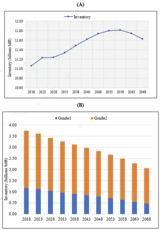
Figure 2.
Projected white oak timber outlook in Kentucky: (A) timber inventory of sawlog volume of white oak trees in the forest; (B) high-quality white oak inventory in the forest [10].
The economy-wide impact of timber supply has been modeled using the CGE framework in a number of studies [11,12,13,14,15,16]. This study supplements and extends the CGE literature on timber supply impacts analysis in several ways. First, this would be the first study to model the economy-wide impacts of white oak timber supply using a CGE model in Kentucky. The state produces 95% of the world’s bourbon; hence, it is of paramount significance to understand how white oak timber supply changes might impact the bourbon industry and the state’s economy. Second, this would be the first study to incorporate the timber quality aspect in an economic impact assessment using the CGE modeling framework. Results from this study will help stakeholders—woodland owners, forest industry, and distillery industry, understand the potential impacts of white oak timber supply on the state’s economy and underscore the urgency of future forest management policies aimed at addressing sustainable white oak management practices in Kentucky and beyond.
The primary motivation of this paper has been to shed light on the pivotal role of white oak in bourbon industries amidst sustainability concerns of the species. While the importance of both the species and industries has been understood per se, studies illustrating the nexus between a species with a niche market like white oak and the associated economic impacts have been lacking. Redressing this research gap is much needed to furnish science-based explanations on the action plan of coalitions like The White Oak Ini-tiative, which brings together white oak-dependent stakeholders to ensure long-term sustainability of the nation’s white oak. Recently, the US House of Representatives introduced H.R.5582, called the White Oak Resilience Act. Hence, our study fits into the larger picture of enhancing communication, coordination, and collaboration on the white oak restoration initiative across the white oak-growing region; the conceptual framework of this study, on the other hand, could serve as a template for future studies at a much broader scale.
The remainder of this article is organized as follows: Section 2 describes the CGE materials and methods used to model the timber supply and the associated economic impacts; Section 3 provides the results of the analysis; Section 4 presents a discussion of the findings and limitations; and, finally, Section 5 concludes the article with some policy recommendations.
2. Materials and Methods
2.1. CGE Model Specifications
We developed a single-region, recursive dynamic CGE model for the economy of Kentucky to examine economy-wide impacts of increased stumpage payments in the wood products sector and decreased barrel expenditures in the distilleries sector due to the increasing timber supply of white oak sawlogs and decreasing timber supply of high-quality white oak sawlogs (suitable for barrels production) in the Commonwealth, respectively.
We specified a CGE model based on neoclassical economic theory, following Ochuodho and Lantz [16] in structure for a single region. We calibrated the model using the 2018 Input–Output (IO) database for Kentucky (Table A1). The model was formulated as a set of simultaneous linear and nonlinear equations defining the behavior of economic agents (households, firms, banks, and rest of the world), market clearance, macroeconomic closures, intertemporal components, and a steady-state economic growth path. Detailed descriptions of model variables, parameters, and equations are provided in Table A2, Table A3 and Table A4, and equation numbers from Table A3 are in parentheses in the paragraphs that follow (below) where appropriate.
In line with a neoclassical model, our model assumes that the economy of Kentucky is so small that it does not exert any influence on the world price of exports and imports. On the import (demand) side, the domestic consumers discriminate between the domestically produced and imported goods through the constant elasticity of substitution (CES) Armington specification (Equations (A18) and (A19)). The final ratio of imports to domestic goods is determined by the relative prices of each type of good, as domestic demanders choose between domestic (within state) and imported (from other states and outside the US) commodities based on their cost-minimizing decisions. Thus, an increase in the domestic–import price ratio causes an increase in the import–domestic demand ratio. The zero-profit condition of the domestic firm (Equation (A20)) suggests that the total value of composite goods (domestic plus foreign) sold in the domestic market must be equal to the sum of the total value of domestic goods sold in the domestic markets and the total value of aggregated imports factored by the world import price and exchange rate and adjusted for tariffs (where applicable) (Equation (A21)).
On the export (supply) side, the domestic firm or producer has the choice between selling its commodity in the domestic market or exporting to foreign markets. Profit maximization drives producers to sell their output in markets where they can maximize profit. The decision of domestic firms is governed by a constant elasticity of transformation (CET) function, which differentiates between exported and domestic goods (Equations (A22) and (A23)). As producers seek a higher returns source, an increase in the export–domestic price ratio causes an increase in the export–domestic demand ratio. The zero-profit condition of the domestic firm (Equation (A24)) suggests that the total value of domestically produced goods must be equal to the sum of the total value of domestic goods sold in domestic markets and the total value of aggregated exports factored by the world export price and exchange rate and adjusted for export tax (where applicable) (Equation (A25)). A balance of payments is established by equating aggregate imports to aggregate exports plus foreign savings at world prices [12]. A zero global trade balance ensures that the values of bilateral trade flows are cleared (Equation (A26)).
On the input side, our model assumes producers as profit maximizers, combining four factors of production (labor, capital, stumpage, and barrel expenditures) with constant returns to scale technology. While most CGE models typically specify only labor and capital as input factors, including stumpage as an input factor follows that of Ochuodho and Lantz [16]. Typically, stumpage payments are recorded in IO tables and a social accounting matrix as part of capital expenditures [16]. While distillery industries purchase barrels on an annual basis, these purchases are not recorded as intermediate inputs but as “capital” expenditures since it takes a number of years to mature bourbon in these barrels (Pers. Comm. with IMPLAN personnel). It therefore makes sense to specify barrel purchase expenditures as an additional input factor. We disaggregated both stumpage and barrel expenditures from capital using external data and an ad hoc approach, which is explained in the model calibration section below.
Producers face a nested production function specified through two levels: at the first level, there is a Leontief technology comprising a composite of value added and a composite of intermediate inputs; at the second level, factors of production are combined through a constant return to scale CES technology (Equation (A1)). The zero-profit condition of the domestic firm (Equation (A2)) suggests that the total value of domestic production must be equal to the sum of the total value of factors of productions and the total value of intermediate productions, which is obtained with factoring the total value of domestic productions by technical coefficients. While labor and capital are mobile among sectors, stumpage is specific to the wood products sector and barrel expenditures to the distilleries sector. The supplies of factor inputs are fixed and exogenously specified in the model based on existing data (see the model calibration section for details). Figure 3 illustrates the nested production structure of the CGE model.

Figure 3.
Nested production structure of the CGE model [author’s illustration].
On the income side, households receive income (Equation (A3)) from supplying factors of production and from import tariff revenues from the domestic government (Equation (A10)). Household savings (Equation (A4)) are a fixed proportion of their total income, as determined by marginal propensity to save. Thus, it is the disposable income (Equation (A5)) that is spent on the consumption of a basket of commodities. The optimal allocation between the consumption of commodities by household, after attaining the minimum subsistence level, is achieved through maximization of a Stone–Geary utility function through a linear expenditure system (LES) subject to disposable income constraint (Equation (A7)). Under this system, the supernumerary income (Equation (A6))—the income remaining after the consumer has purchased the minimum required quantities of commodities—is allocated over commodities based on fixed proportions (marginal budget shares). Total savings in the economy are the sum of household savings and foreign savings factored by the exchange rate (Equation (A8)).
In the final demand, the investment demand by the banks is determined by the total savings factored by the Cobb–Douglas investment preference for each commodity (Equation (A9)). A Phillips curve is specified in the model to introduce involuntary unemployment (Equation (A11)). This explains the wage–unemployment relationship in the model using factor prices and supplies and the Laspeyres consumer price index (CPI) (Equation (A12)).
Equilibrium in the factor market requires that the demand for factors equals the supply. To achieve equilibrium, factor prices in the market must adjust to ensure that demand equals supply. However, due to an imperfect labor market, there is involuntary unemployment; therefore, market clearing in the labor market is relaxed to allow for unemployment in labor supply (Equations (A13)–(A16)). Equilibrium in the commodities market requires that demand for commodities equals supply. Aggregate demand for each commodity comprises household consumption spending (consumption, investment, and intermediate) on domestic and imported goods. Aggregate supply includes both domestic production and imported goods (Equation (A17)). All prices of commodities (except import price when there is tariff) and primary factors are normalized to unity in the initial equilibrium. Given that prices are normalized to one, the “values” in the IO accounts can be interpreted as physical quantity indices per unit of currency in the commodity and factor markets. This procedure converts most of the initial, or base, prices in the model into USD 1. It means most prices (unless we have taxes or subsidies) in a CGE model have an initial level value of 1 and those values deviate from 1 following a dynamic growth path and/or the shocks imposed. This practice of normalizing data considerably reduces the information required to build a CGE model database without compromising the capability of the model to generate results for prices, quantities, and values [17].
The CGE model is solved under the “square matrix condition”, i.e., the number of single endogenous variables must equal the number of single equations. To achieve this condition, the model closure has to be specified in a way to ensure mathematical solvability while reflecting reality reasonably and meeting the modeler’s needs depending on the context of the analysis [18]. To achieve this, we exogenously fixed factor supplies and foreign savings while rendering the exchange rate adjustable. Foreign savings are set as the difference between the value of exports and the value of imports. The wage rate is exogenously fixed as the numeraire price [12]. An artificial objective function is included to help the model solve.
2.2. Model Calibration
The model was calibrated using the 2018 baseline symmetric Input–Output (IO) table database for Kentucky that was obtained from the Input–Output—State and National Analysis Program (IO-SNAP), obtained from the Regional Research Institute (RRI) at West Virginia University. The original 70 industries in the IO table were aggregated into 11 sectors (Table 1) for convenience. Four primary factors of production were specified: labor, capital, stumpage (specific to wood products manufacturing), and barrel expenditures (specific to the distilleries sector). Labor was measured as an employee’s compensation in the IO table. Capital was aggregated as the sum of taxes of production and imports, other subsidies, and gross operating surplus in the value-added account of IO table. Typically, CGE models require additional data that are not contained in IO tables. Therefore, such data must be obtained from other sources. There are also some plausible assumptions that are made in the model calibration process, which is typical of most economic models. Stumpage in the wood products sector and barrel expenditures in the distilleries sector were not identified as input factors in the original IO table. Instead, these payments are embedded in each sector’s “other operating surplus” as a part of capital [16] (Pers. Comm. with IMPLAN personnel, 2020). Since these payments were not readily available for Kentucky, we used an ad hoc approach to isolate them from the capital in the wood products and the distilleries sectors, respectively.

Table 1.
Production sectors included in the CGE model.
To isolate stumpage payments for the wood products manufacturing sector, we relied on information from other sources. According to the Kentucky Forest Sector Economic Contribution Report 2018, 731 million board feet of hardwood logs were harvested in Kentucky in 2018, with the woodland owners receiving, on the statewide average, USD 0.29 per board feet. This would give a statewide average stumpage payment of USD 211.99 million in 2018. Since Kentucky produces predominantly hardwood—more than 80% of timber harvested in 2018 was hardwood [2]—we assumed that the estimated average stumpage payment was representative of the total statewide stumpage payments in 2018. As our species of interest was white oak only, we used the 2018 timber product output (TPO) data for Kentucky to tease out stumpage payment for the white oak species, assuming that stumpage payments are equal to the proportion of timber harvested by product type and species group. According to the TPO data [2], about 91% of hardwood logs harvested in 2018 were sawlogs, of which about 16% belong to the select white oak species group. In this way, we estimated the statewide average stumpage payments as about USD 31 million for white oak sawlogs in Kentucky and subtracted the stumpage value from capital in the wood products sector.
Barrel expenditures by distilleries were also isolated using information from external sources. According to a report [6], about 1.7 million barrels of new bourbon were produced and added to warehouse inventory in Kentucky in 2018. Since a 53-gallon American white oak barrel is a standard size mostly used in all local Kentucky distilleries, with distillers paying, on average, USD 190 (personal communication of proprietary information from cooperage and distilling industries) for a high-quality white oak barrel, we estimated the barrel expenditures for distilleries to be about USD 323 million in 2018. This barrel expenditure was disaggregated from capital expenditures in the distilleries sector.
A suite of parameters is required to calibrate the model using the IO dataset. Endogenous parameters such as share and shift parameters were calibrated endogenously from the Input–Output data. Income elasticities of demand for commodities were obtained from [19]. Armington, CET, and CES elasticities were obtained from an earlier CGE model [14,16], which had been derived from the Global Trade Analysis Project (GTAP) database following sectoral aggregations. In addition, elasticities for some commodities were borrowed from [20]. The annual state unemployment rate was obtained from Kentucky’s labor force estimates [21].
The model is first formulated as a static model that meets standard technical tests for a well-specified CGE model. With a well-specified static model, a recursive dynamic path was specified for the 40-year (2018–2058) projection horizon. For every period, capital stock is updated via a capital accumulation equation based on an endogenous growth rate determined by the return on capital rate and endogenous total savings (Equations (A31) and (A32)) [13,22]. Labor is assumed to grow exogenously in the model. Assuming that labor supply growth projections are consistent with projected population trends (Ochuodho and Lantz 2014), we estimated annual labor supply growth rates from Kentucky population projections between 2015 and 2040 for both sexes and all ages [23]. Stumpage payment and barrel expenditures were exogenously fixed at 2018 levels over time under baseline conditions. Holding these variables constant is consistent with other related studies that specified stumpage as an input factor [16]. All present-value calculations were evaluated in nominal-value (2018) US dollar terms using a 4% nominal discount rate; this rate approximates the average annual discount rate for the US over the 1983–2018 period [24].
2.3. Model Solutions and Simulations
The model equations were solved using the General Algebraic Modeling System (GAMS 28.2.0) software as a nonlinear programming (NLP) problem using appropriate algorithm codes along with CONOPT4 solver [25]. After solving the model for the initial period equilibrium to replicate the 2018 benchmark IO data, a dynamic baseline growth path of the economy was simulated in the model following the growth path described above. This baseline scenario is otherwise known as the “business as usual” (BAU) path.
In the simulation scenario run, we considered economic impacts of the projected white oak timber supply (Table 2). Specifically, we targeted how the projected white oak timber supply would affect the wood products manufacturing and distilleries sectors. The wood products sectors rely on white oak sawlogs for manufacturing myriad primary and secondary wood products while the distilleries sector relies on high-quality white oak sawlogs for barrel manufacturing, a prerequisite for bourbon production. The supply (demand) of white oak sawlogs is captured in the model in the wood products sector by the stumpage paid by the sector, and the supply (demand) of high-quality white oak sawlogs is captured in the distilleries sector by the barrel expenses made by the sector, as only high-quality white oak stave logs are used for barrel manufacturing. The 40-year trend of both variables are based on results of an earlier study [9]. To capture these trends in the CGE model, we are using stumpage payment as a proxy of white oak sawlog supply and barrel expenditures as a proxy of high-quality white oak sawlogs supply (primary input). We are, thus, assuming that stumpage will be increased by the same percentage as the annual supply of white oak sawlogs and barrel expenditures will be reduced by the same percentage as the annual supply of high-quality white oak sawlogs (Table 2) from 2018 to 2058. It is possible that as there is more availability of sawlogs overall for the wood products sector but less availability of high-quality sawlogs for the distilleries sector, the stumpage price may fall, and the barrel price may rise, and revenues may not fall/rise by the same amount as the fall/rise in timber supply. However, understanding the exact impact on prices is beyond the scope of this study, particularly since stumpage and barrel expenditures are exogenous in the model. With the current methodology, we were able to capture the impact of the rise in stumpage payments due to the rise in demand of white oak sawlogs (the attraction of new wood products mills and expansions of existing ones) and the impact of the decline in barrel expenditures due to the fall in supply of high-quality white oak sawlogs (reduction in payments by barrel producers): two main goals of this study. Corbett et al. [14] employed a similar assumption and modeling approach in assessing the economic impacts of reduced timber supply resulting from a mountain pine beetle infestation in British Columbia, Canada.
Table 2.
Summary of Kentucky input changes simulated in the CGE model.
The average annual stumpage expenditure increments amounted to 0.22% (2018–2058) for the timber supply simulation relative to the baseline. The average annual reduction in barrel expenditures amounted to −0.82% (2018–2058) for timber supply simulation relative to the baseline. Since stumpage and capital expenditures on barrels are exogenous in the model, prices are endogenously determined by the model under general equilibrium conditions. Both stumpage supply and barrel expenditures simulations were implemented simultaneously. Differences in economic variables’ levels between simulation shock and BAU give the economy-wide impacts of the simulated shocks.
3. Results
Table 3 provides a summary of the economy-wide impacts of the projected supply of white oak timber as simulated through increased supply of white oak sawlogs for the wood products sector and reduced supply of high-quality white oak sawlogs for distilleries for bourbon barrels manufacture. Table 3 presents both levels (discounted cumulative dollar values) and percent-change impacts of the simulated shocks of timber supply, as captured by the overall increase in stumpage and decline in barrel expenditures over a 40-year period (2018–2058).
Table 3.
Discounted cumulative impacts (USD billion) of timber supply simulation relative to the baseline scenario (2018–2058).
Overall and as expected, the economic impacts for most of the key macroeconomic variables were negative. This is because the magnitude of the simulated negative shock we imposed was higher than the positive shock. The overall negative economic impacts of the simulated shocks are mostly driven by the negative shock imposed on the distilleries sector, which had three-times (USD 6 billion) of total output to that of the wood products sector (USD 2 billion) in 2018 (based on the original IO database). As a result, the negative economic impacts are mostly driven by declining annual barrel expenditures in the distilleries sector, consistent with the declining supply of high-quality white oak sawlogs during the projected timeframe.
The negative GDP impacts were driven by the negative impacts of its component elements, including consumption, net exports, and investment. Shocks to stumpage payments in the wood products sector and barrel expenditures in the distilleries sector impacted intermediate and final demand consumptions in each sector, as well as in all other sectors through feedback effects (direct, indirect, and induced impacts), hence the economy-wide impacts. As production in the distilleries sector declined due to declining supply of high-quality white oak sawlogs (a factor of production), it had a spillover effect on domestic output/production of some other sectors, such as agriculture (−0.19%) and transportation (−0.07%), that are indirectly related to supplies in the distilleries sector. Consequently, the overall decline in domestic production led to the overall rise in commodities’ price, hence the reduction in overall consumption. The percentage change in variables such as domestic production (output), consumption, and income followed a similar pattern to that of GDP.
In response to the simultaneous stumpage and barrel expenditures shocks, Kentucky’s GDP reduced by a cumulative discounted value of around USD 3.66 billion (−0.085%), which averages approximately USD 91 million annually from 2018 to 2058. To put it into perspective, a USD 91 million reduction is equivalent to roughly 40% of statewide stumpage payments in 2018. The GDP reduction is driven by reductions in final demand components, including consumption (−0.011%) and exports (−0.103%), as well as reduction in household income (−0.12%) and domestic production (−0.031%), particularly production in the distilleries sector (−1.308%) on the input side, which constituted 0.8% of state’s GDP in 2018 (derived from Table A1). For the timber supply simulation, the cumulative present value of household income, consumption, exports, total domestic production, and distilleries production were simulated to decrease by USD 5.14 billion (USD 128 million annually), USD 0.36 billion (USD 9 million annually), USD 1.61 billion (USD 40 million annually), USD 2.33 billion (USD 58 million annually), and USD 0.57 billion (USD 14 million annually), respectively. To gain some perspective, a USD 128 million annual reduction in household income is roughly equivalent to the Commonwealth’s entire exports of barrels in 2018. Tracing the causal paths further, some of the estimated impacts on key macroeconomic variables can be explained in relation to price changes, which are determined endogenously in the model. The reduction in domestic production of the distilleries sector because of the shock we imposed in its factor of production drove the overall reduction in domestic production (−0.031%) under the timber supply shock simulation, and eventually income (−0.12%). As overall domestic production declined due to supply constraint, the supply price of domestically produced commodities rose (0.052%). Since the supply could not keep up with the domestic demand of commodities, the demand price of commodities rose (0.146%), which eventually led to a decline in household consumption of commodities. Similarly, the price of the domestically produced commodities delivered to domestic markets grew by 0.288%, while the export prices fell by 0.076%. Consequently, exports fell by 0.103% under the shock simulation as foreign markets became less profitable for the producers relative to the domestic market. This is a typical constant elasticity of transformation (CET) reaction, governing the producer decision on where to sell (domestic or foreign market). The producer’s decision to allocate production between domestic and foreign markets depends on the relative prices in the two markets. A change in the nominal exchange rate variable, expressed in terms of the currency of the exporting region, will change the fob export price in the domestic currency that is received by producers of the exported good [17].
Consumer welfare, measured with compensating variation (CV), declined due to the timber supply shock, with the cumulative present value of CV approximating USD 149 billion over the 40-year horizon. It means that under the timber supply simulation shock, the consumer would be worse off by roughly USD 706 million relative to the baseline scenario. As a frame of reference, USD 706 million is roughly equivalent to the direct economic contribution of the pulp and paper sector in 2018 in Kentucky. The welfare losses can be explained with the change in utility following the simulation shock. Utility is essentially the function of commodities’ prices and consumer income levels. As the overall demand in factors of production declined due to the shocks imposed, consumer income fell by 0.12%. In addition, as discussed earlier, the price of commodities rose by 0.146% following timber supply simulation. Consequently, utility fell by 0.036% under the timber supply scenario, which means the consumer would require an additional USD 706 million to reach the original utility level at baseline before the timber supply shock.
In terms of inputs to production, labor expenditures increased by USD 1.14 billion (0.047%). An explanation for this result would be the mobility of factors across sectors specified in our model, thereby compensating the reduction in labor expenditure in the distilleries sector by a shift in labor demand in other sectors. Furthermore, as the demand price of commodities rose (0.146%), demand for commodities in the domestic market fell (−0.016%); as a result, imports fell by 0.134%.
Since our sectors of interest were wood products and distilleries only, we isolated stumpage payments in the wood products sector and barrel expenditures in distilleries as additional factors of production beside labor and capital. For the rest of the sectors, including forestry and logging, there were only two factors of production. In this regard, the change in white oak log supply is not reflected in terms of the forestry and logging sector. However, because each and every sector in an economy is connected in the CGE models, we can trace the impact of scenario or policy changes in every sector. Table 4 summarizes the discounted cumulative impacts (both in USD billion and %) on total outputs for the rest of the nine sectors. These impacts on residual sectors can be viewed as an indirect impact of the projected white oak timber supply in the wood products and distillery sectors. The forestry and logging sector, in particular, is estimated to have a positive economic impact, with the cumulative output of USD 5 million over the next 40 years. This could be ascribed to the wood products sector’s intermediate inputs (around USD 45 million) from the forestry and logging sector in their own production process (Table A1). Because production is a composite of value added and intermediate inputs, the positive economic impact in the forestry and logging sector is the ripple effect of the positive economic impacts of USD 151 million in the wood products output (Table 3).
Table 4.
Summary of the discounted cumulative impacts of timber supply simulation relative to the baseline scenario (2018–2058) on total outputs for the rest of the nine sectors in Kentucky.
4. Discussion and Limitations
In this study, we were able to capture both direct (sectors of interest) and induced (overall economy) dynamic impacts of the projected white oak timber supply using a CGE model for Kentucky based on the projected inventory levels. The findings of this work provide estimates of the economy-wide impacts of increasing supply of white oak sawlogs and the simultaneous decline in supply of high-quality white oak sawlogs in Kentucky. Overall, our findings suggest a negative economy-wide impact in Kentucky. The macroeconomic indicators show that the GDP would reduce by USD 3.66 billion, consumption by USD 363 billion, and exports by about USD 1.61 billion in terms of the cumulative present value. Additionally, consumer welfare would decline by about USD 700 million. Furthermore, most of the sectoral outputs would contract—notably distilleries, manufacturing, and agriculture—over the simulation horizon of 40 years. While we are ordinarily using an established analytical approach in assessing the economy-wide impacts with just a few customized specifications, the novelty of our study is the application of the CGE model in addressing a timely issue of greater relevance for Kentucky’s bourbon industries. Using an economic tool, this study provides new insights to forest industries, especially distilleries, regarding the direct and indirect economic effects of the white oak resource on regional economies and hopes to foster dialogue on white oak conservation programs among dependent stakeholders across the nation.
Results of this study are consistent with similar studies that used a dynamic, single-region CGE model. Chang et al. [13] employed a dynamic CGE model to assess the potential impacts of future spruce budworm (SBW) outbreaks in New Brunswick from 2012 to 2041. Under a severe SBW scenario, the total output in present-value terms was found to decline by USD 4.7 billion, with negative economy-wide impacts in terms of output, returns of labor, and capital. Corbett et al. [14] imposed a stumpage shock in the forest sector, reflecting the fall in the annual allowable cut due to a mountain pine beetle infestation in British Columbia from 2009 to 2054; the study estimated the reduction in the cumulative discounted value of the GDP, household income, CV, consumption, imports, exports, total domestic production, and forestry sector production.
A model is only as good as its assumption. Like any model, CGE model results are sensitive to the assumptions upon which it is built; therefore, altering the assumptions will most likely change the magnitude of the impacts. First and for simplicity, we assumed that white oak supply is equal to white oak inventory. However, biophysical (physiography, slope, and stand size) and social constraints (distance to road, landowners’ intent to harvest, and parcel size) could reduce the actual market supply of white oak timber, further increasing the magnitude of economic impacts. Second, the forestry and logging sector was not constrained in the sense that stumpage was restricted to the wood products manufacturing sector only. Third, the model is deterministic in nature, i.e., the economic agents have perfect foresight of future white oak product supply and there is no change in market demand for white oak lumber products and barrels over the projection horizon. This may not be the actuality, as we know the market can be affected by various exogenous shocks such as the business cycle, and taste and preferences. Fourth, parameters such as elasticities are assumed to be the same as those in other national/regional-level studies. The lack of state/sector-specific parameters is a widely cited concern regarding CGE models, as results tend to be sensitive to the parameters upon which the model is calibrated [11,16]. However, it is worth noting that elasticities are based on industries’ economic structures and production technology, which are more or less similar across states in the US. Fifth, there is no trade among adjacent white oak-growing states such as Missouri and West Virginia, which can have feedback effects on Kentucky’s economy. A multi-regional CGE model, unlike our single-region model, would have captured this.
The aforementioned assumptions of the CGE model could affect the magnitude of the estimated economic impacts in either direction. For instance, because the overall negative impact is driven by the higher rate of reduction in the high-grade white oak timber consumed by relatively larger distillery sectors (in terms of economic outputs), further reduction in the harvestable white oak resource base due to biophysical and social constraints could drive up the average annual reduction in high-quality white oak timber, thus augmenting the overall negative economic impacts as measured by key macroeconomic variables in the model. However, relaxation of elasticity parameters (especially own-price elasticity) and allowing trade among adjacent white oak-growing states could offset the overall negative economic impacts to some extent (increasing distilleries’ output, consumption, income, GDP, and welfare). Thus, interpretation of CGE results must be pegged on the underlying model assumptions.
Further, in interpreting our results (Table 3), it is worth noting that the Input–Output database used in the CGE model is highly aggregated. The database is not disaggregated enough to provide “lower-level” information on all primary and secondary forest industries that use white oak sawlogs in their production process (intermediate demand) such as pallets, railroad ties, stave logs for barrels, and sawlogs for lumber separately. Consequently, while the stumpage expenditures in the wood products sector are increasing due to increasing demand of white oak timber, stumpage expenditures in some of the secondary wood manufacturing industries might be decreasing. In addition, because the decline in white oak timber supply only occurs during the last ten years of the planning horizon (2058–2068), the wood products sector experiences positive impacts (realized between 2018 and 2058: Figure 2) while the distilleries sector experiences only marginal negative impacts. Since the decline in timber supply starts to occur much later, the impacts are only marginal in discounted present-value terms (Table 3).
Our results must be interpreted in the context of this study. For now and in the next few decades (2018–2058), there is no “crisis” of white oak timber supply per se. However, starting 2058, the sustainability of white oak timber supply becomes critical for the sectors that depend on it. Given the long rotation of white oak high-quality stave logs, this projected decline should be addressed today by implementing policies that would encourage white oak regeneration and recruitment. This is where management policy incentives for private forestland owners and conservation programs come into play. Such incentives to avert the projected decline in white oak timber supply will ultimately benefit the entire economy of Kentucky given the interconnectedness of all sectors of the economy. The distilleries sector, which directly depends on the sustained supply of high-quality white sawlogs, interacts with all other sectors through, direct, indirect, and induced impacts. For instance, the distilleries sector, which is heavily dependent on white oak sawlogs, has three-times the economic output to that of the wood products sector. Therefore, any impacts that affect this output will ultimately have effects on other sectors of the economy.
The estimates reported here are just that: estimates. Given the scale at which this study was conducted, and the level of exogenous data required to build a comprehensive CGE model, there are some obvious limitations as well as possibilities for future analysis. First, the IO database is susceptible to aggregation bias. Additionally, the problem of not having disaggregated sectors is aggravated by the lack of data on the stumpage or timber product output of white oaks that would go into each of those primary and secondary wood manufacturing sectors. Having a more detailed and disaggregated IO table with such details would minimize the errors and inconsistencies that might occur when such data are derived externally. Second, readers should keep in mind that CGE simulations are like controlled thought experiments of “what if” scenarios in an experimental world [26]; it is therefore not practical that the real world (with ever-changing events) will be responding in an exact manner at an exact time, as predicted by the model. We acknowledge that there is a lack of region/sector-specific data for various calibration parameters in the CGE model such as elasticities, Frisch, and the Phillips curve. CGE model results tend to be sensitive to the parameters upon which the model is calibrated. Our elasticities are sourced from related previous studies in Canada and the US. While region- and sector-specific elasticities are preferred, generating such elasticities is a whole study by itself as it requires panel data spanning many years. CGE modeling studies typically use sourced elasticities rather than generate region-specific ones every time. Further, our single-region CGE model does not consider how white oak timber supply changes in other states may affect trade (import/exports) in Kentucky; a multi-regional CGE model that captures such impacts would be needed for this, which is an area for future research.
5. Conclusions and Policy Recommendations
The results presented in this study are valuable first estimates that can be used to advocate for proactive forest management practices to stabilize and streamline a sustained supply of high-quality white oak timber in Kentucky and beyond, against the economic consequences of the status quo if nothing is done. Since the impacts are mostly negative, this study highlights the economic implications of a sustained supply of high-quality white oak sawlogs, which has direct relevance to the ongoing White Oak Initiative spearheaded by the University of Kentucky’s Department of Forestry and Natural Resources. By demonstrating the potential economy-wide impacts of decreasing the supply of high-quality white oak sawlogs, this study stresses the urgency of the white oak sustainability issue as well as calls for swift policy and/or management intervention, bringing together white oak-dependent stakeholders to coordinate, develop, and implement sustainable white oak management practices in Kentucky and beyond.
The coalition of partners such as the establishment of the White Oak Initiative and the formation of the Congressional White Oak Caucus can play a critical role in long-term white oak sustainability and dependent industries through developing, coordinating, and implementing policies geared towards sustainable oak management practices. Dissemination of science-based forest management practices from state agencies and university extensions and government cost-share assistance programs to non-industrial private forestland owners through participation in state-supported property-tax incentive programs like the Classified Forest and Wildland Program in Indiana and federal assistance programs like the Environment Quality Incentives Program, could be better implemented to promote white oak management and quality.
Author Contributions
Conceptualization, G.D. and T.O.O.; methodology, G.D. and T.O.O.; software, G.D. and T.O.O.; validation, G.D. and T.O.O.; formal analysis, G.D. and T.O.O.; investigation, G.D.; resources, T.O.O.; data curation, T.O.O.; writing—original draft preparation, G.D.; writing—G.D. and T.O.O.; visualization G.D.; supervision, T.O.O.; project administration, T.O.O.; funding acquisition, T.O.O. All authors have read and agreed to the published version of the manuscript.
Funding
This research was funded by the USDA National Institute of Food and Agriculture, McIntire-Stennis Project Number 1018771.
Data Availability Statement
Data available on Table A1.
Conflicts of Interest
The authors declare no conflicts of interest.
Appendix A
Table A1.
Input–Output database for Kentucky, 2018 (USD billion).
Table A2.
CGE model variables.
Table A3.
CGE model parameters.
Table A4.
CGE model equations.
References
- USDA Forest Service. EVALIDator Version 1.8.0.01 [WWW Document]. For. Invent. Anal. Program, North. Res. Station. St. Paul, MN. 2020. Available online: https://apps.fs.usda.gov/Evalidator/page5tmfiltersPost.jsp (accessed on 15 July 2020).
- USDA Forest Service. Timber Product Output and Use for Kentucky, 2018; Resour. Update; FS-285; U.S. Department of Agriculture, Forest Service: Asheville, NC, USA, 2020; 2p.
- Office of the Federal Register. Code of Federal Regulations [WWW Document]. Fed. Regist. 2018. Available online: https://web.archive.org/web/20180318072452/https://www.ecfr.gov/cgi-bin/text-idx?SID=57b5394734f53825e7e126b2cf0883bb&mc=true&node=se27.1.5_122&rgn=div8 (accessed on 21 January 2021).
- Conner, J.; Reid, K.; Jack, F. Chapter 7—Maturation and blending. In Whisky, Handbook of Alcoholic Beverages; Russell, I., Russell, I., Bamforth, C.W., Stewart, G.G., Eds.; Academic Press: San Diego, CA, USA, 2003; pp. 209–240. [Google Scholar] [CrossRef]
- White Oak Initiative. Restoring Sustainability for White Oak and Upland Oak Communities: An Assessment and Conservation Plan. 2021. Available online: https://static1.squarespace.com/static/5cd1e6d5f9df7d00015ca6a4/t/625eadbba49a066a88e68e9d/1650372118921/White-Oak-Initiative-Assessment-Conservation-Plan.pdf (accessed on 21 December 2023).
- Coomes, P.; Kornstein, B. The Economic and Fiscal Impacts of the Distilling Industry in Kentucky; Kentucky Distillers’ Association: Frankfort, KY, USA, 2019. [Google Scholar]
- Nowacki, G.J.; Abrams, M.D. The Demise of Fire and “Mesophication” of Forests in the Eastern United States. Bioscience 2008, 58, 123–138. [Google Scholar] [CrossRef]
- Abrams, M.D. Where has all the White Oak gone? Bioscience 2003, 53, 927–939. [Google Scholar] [CrossRef]
- Dhungel, G.; Poudel, K.; Ochuodho, T.O.; Lhotka, J.M.; Stringer, J.W. Sustainability of White Oak (Quercus alba) Timber Supply in Kentucky. J. For. 2023, fvad041. [Google Scholar] [CrossRef]
- Gadzik, C.J.; Blanck, J.H.; Caldwell, L.E. Timber Supply Outlook for Maine: 1995–2045; Forest Service Documents; Maine Department of Agriculture, Conservation and Forestry, Maine Department of Conservation, Maine Forest Service: Augusta, ME, USA, 1998; 39p.
- Das, G.G.; Alavalapati, J.R.R.; Carter, D.R.; Tsigas, M.E. Regional impacts of environmental regulations and technical change in the US forestry sector: A multiregional CGE analysis. For. Policy Econ. 2005, 7, 25–38. [Google Scholar] [CrossRef]
- Zhang, J.; Alavalapati, J.R.R.; Shrestha, R.K.; Hodges, A.W. Economic impacts of closing national forests for commercial timber production in Florida and Liberty County. J. For. Econ. 2005, 10, 207–223. [Google Scholar] [CrossRef]
- Chang, W.Y.; Lantz, V.A.; Hennigar, C.R.; Maclean, D.A. Economic impacts of forest pests: A case study of spruce budworm outbreaks and control in New Brunswick, Canada. Can. J. For. Res. 2012, 42, 490–505. [Google Scholar] [CrossRef]
- Corbett, L.J.; Withey, P.; Lantz, V.A.; Ochuodho, T.O. The economic impact of the mountain pine beetle infestation in British Columbia: Provincial estimates from a CGE analysis. Forestry 2016, 89, 100–105. [Google Scholar] [CrossRef]
- Karttunen, K.; Ahtikoski, A.; Kujala, S.; Törmä, H.; Kinnunen, J.; Salminen, H.; Huuskonen, S.; Kojola, S.; Lehtonen, M.; Hynynen, J.; et al. Regional socio-economic impacts of intensive forest management, a CGE approach. Biomass Bioenergy 2018, 118, 8–15. [Google Scholar] [CrossRef]
- Ochuodho, T.O.; Lantz, V.A. Economic impacts of climate change in the forest sector: A comparison of single-region and multiregional CGE modeling frameworks. Can. J. For. Res. 2014, 44, 449–464. [Google Scholar] [CrossRef]
- Burfisher, M.E. Introduction to Computable General Equilibrium Models, 2nd ed.; Cambridge University Press: New York, NY, USA, 2016. [Google Scholar]
- Lofgren, H.; Harris, R.L.; Robinson, S. A Standard Computable General Equilibrium (CGE) Model in GAMS, Microcomputers in Policy Research 5; International Food Policy Research Institute: Washington, DC, USA, 2002. [Google Scholar]
- Dimaranan, B.V. The GTAP 6 Data Base; Center for Global Trade Analysis, Department of Agricultural Economics, Purdue University: West Lafayette, IN, USA, 2006. [Google Scholar]
- Thurlow, J.; van Seventer, D.E.N. A Standard Computable General Equilibrium Model for South Africa, Trade and Macroeconomics Discussion Paper No. 100; International Food Policy Research Institute: Washington, DC, USA, 2002. [Google Scholar]
- Kentucky Center for Statistics. State Releases Annual County Unemployment Data for 2018 [WWW Document]. 2019. Available online: https://kystats.ky.gov/KYLMI/PressRelease?id=70a7996d-2b44-412f-9dc1-686c9895a609 (accessed on 8 March 2021).
- Alfsen, K.H.; De Franco, M.A.; Glomsrød, S.; Johnsen, T. The cost of soil erosion in Nicaragua. Ecol. Econ. 1996, 16, 129–145. [Google Scholar] [CrossRef]
- Kentucky State Data Center. Preliminary Kentucky Population Projections; University of Louisville: Louisville, KY, USA, 2016; pp. 2015–2040. [Google Scholar]
- International Monetary Fund. Interest Rates, Discount Rate for United States [WWW Document]. Fed. Reserv. Econ. Data, Fed. Reserv. Bank St. Louis. 2018. Available online: https://fred.stlouisfed.org/series/INTDSRUSM193N (accessed on 22 March 2021).
- GAMS. General Algebraic Modeling System; GAMS Development Corporation: Washington, DC, USA, 2012. [Google Scholar]
- Hertel, T.W.; Keeney, R.; Ivanic, M.; Winters, L.A. Distributional Effects of WTO Agricultural Reforms in Rich and Poor Countries. Econ. Policy 2007, 22, 291–337. [Google Scholar] [CrossRef][Green Version]


Disclaimer/Publisher’s Note: The statements, opinions and data contained in all publications are solely those of the individual author(s) and contributor(s) and not of MDPI and/or the editor(s). MDPI and/or the editor(s) disclaim responsibility for any injury to people or property resulting from any ideas, methods, instructions or products referred to in the content. |
© 2024 by the authors. Licensee MDPI, Basel, Switzerland. This article is an open access article distributed under the terms and conditions of the Creative Commons Attribution (CC BY) license (https://creativecommons.org/licenses/by/4.0/).