Article

Optimizing China’s Afforestation Strategy: Biophysical Impacts of Afforestation with Five Locally Adapted Forest Types

1
Beijing Meteorological Data Center, Beijing Meteorological Bureau, Beijing 100097, China
2
School of Information, Central University of Finance and Economics, Beijing 100081, China
*
Author to whom correspondence should be addressed.
Forests 2024, 15(1), 182; https://doi.org/10.3390/f15010182
Submission received: 8 December 2023 / Revised: 11 January 2024 / Accepted: 11 January 2024 / Published: 17 January 2024
(This article belongs to the Special Issue Forest Microclimate: Predictions, Drivers and Impacts)

Abstract

:
Recent research has mapped potential afforestation land to support China’s goal of achieving “carbon neutrality” and has proposed tree species selection to maximize carbon uptake. However, it overlooked biophysical climatic effects, which have a more significant impact on local temperature than CO2 reduction. This study aims to present a comprehensive understanding of how afforestation in China affects local and regional climates through biophysical processes. It focuses on the latitudinal patterns of land surface temperature differences (ΔLST) between five locally adapted forest types and adjacent grasslands using satellite-based observations. Our key findings are as follows: Firstly, broadleaf forests and mixed forests exhibit a stronger cooling effect than coniferous forests due to differences in canopy structure and distribution. Specifically, the net cooling effects of evergreen broadleaf forests (EBFs), deciduous broadleaf forests (DBFs), and mixed forests (MFs) compared to grasslands are −0.50 ± 0.10 °C (mean ± 95% confidence interval), −0.33 ± 0.05 °C, and −0.36 ± 0.06 °C, respectively, while evergreen needleleaf forests (ENFs) compared to grasslands are −0.22 ± 0.11 °C. Deciduous needleleaf forests (DNFs) exhibit warming effects, with a value of 0.69 ± 0.24 °C. In regions suitable for diverse forest types planting, the selection of broadleaf and mixed forests is advisable due to their enhanced local cooling impact. Secondly, temperate forests have a net cooling effect to the south of 43° N, but they have a net warming effect to the north of 48° N compared to grasslands. We recommend caution when planting DNFs, DBFs, and MFs in northeastern China, due to the potential for local warming. Thirdly, in the mountainous areas of southwestern China, especially when planting ENFs and MFs, tree planting may lead to local warming. Overall, our study provides valuable supplementary insights to China’s existing afforestation roadmap, offering policy support for the country’s climate adaptation and mitigation efforts.

1. Introduction

China is committed to achieving “carbon neutrality” by 2060, i.e., net-zero carbon emissions [1]. This ambitious goal requires great efforts in both emission reduction and atmospheric CO2 removal [2,3]. Forestation is a crucial climate mitigation strategy, offering substantial potential to capture atmospheric CO2 and store it in plant biomass and soil organic matter. The total forest area in China has rapidly increased since the 1990s [4]. Enhancing the forest carbon sink has been identified as an important component of the national climate mitigation plan [5]. Until now, the Chinese government has set several forest cover targets to expand forest areas [6]. However, forestation could affect the climate directly through the alteration of water vapor, energy, and momentum exchange between the land surface and the atmosphere, known as biophysical climate effects [7,8,9,10]. Such biophysical feedback, resulting in either local cooling or warming, could intensify, diminish, or even reverse the cooling advantages derived from carbon absorption [4,11,12]. Consequently, they are scientifically acknowledged to be significant drivers of climate dynamics. Until now, climate mitigation policies have rarely included biophysical processes, mainly due to their high spatiotemporal heterogeneity.
Recent research has mapped the potential forestation land to support China’s “carbon neutrality” objective and has suggested the tree species selection to maximize local adaptation and carbon uptake [13]. For example, coniferous forests are mostly suitable for Northern China, whereas broad-leaved trees and warm conifers are more apt for Southern China. Though this roadmap effectively supports China’s carbon neutrality progress, it does not consider any biophysical climatic effects, which affect temperature more than CO2 reduction does at a local scale [14].
A series of research advancements have enhanced our understanding of quantifying the influences of forestation on local climates through biophysical pathways, including their latitudinal and seasonal patterns. For example, satellite-based observations showed that the climate effect in mid-latitude forest was mixed [15,16]: the forest showed a cooling effect in the southern temperate zones and a warming effect in the northern temperate zones, when compared with cropland or pasture. The climate feedback of temperate in the forest also varied from season to season. These findings are also supported by studies from the perspectives of energy balance [17] and vegetation indices [18]. However, most researchers have focused on broad categories of forests [15,16,17,18], with limited studies addressing specific forest species. Different types of forests have different canopy structures, which will adapt to the environmental conditions of their latitudinal habitat, such as light, temperature, and water. In turn, through biophysical processes, they feed back, influencing the climate system. For example, conifer canopies are particularly effective in distributing light due to the clumping of their needles around the stems. So, conifer canopies can be distributed in regions with less favorable sunlight conditions, such as those at northern latitudes [19]. On the other hand, deep and uneven canopies of conifer forests typically have a low albedo, causing local warming [20,21]. Therefore, forest types that are ecologically well-suited to the local environment may weaken the cooling advantages of carbon sequestration through their biophysical processes. In light of this, it is beneficial to ask the following questions: (1) In which areas do forest types enhance or diminish the cooling benefits of the carbon sink through their biophysical paths? (2) Are these biophysical climate effects intricately linked with the latitudinal ranges in which the forest types are distributed? If so, how do we explain this correlation? Answering these questions can further deepen our understanding of the impact of afforestation on microclimate conditions, thereby contributing to a more comprehensive assessment of China’s afforestation roadmap to support the country’s climate mitigation policies.
Climate models and in situ measurements are often used to understand how forests affect the climate through biophysical processes. However, large uncertainties exist in these two approaches when addressing this particular problem. Deforestation often takes place in small patches which are difficult for coarse-resolution climate models to capture [15]. For example, climate models could lead to uncertainties surrounding physical processes, parameterization, and biases in land cover classification [22,23]. On the other hand, in situ measurements are relatively sparse, while forest cover change often occurs in areas lacking long-term, reliable meteorological data [12]. Advanced satellite observations can overcome these limitations at the local scale and can provide large-spatial-scale data with consecutive timing and high resolution. Over the past two decades, numerous satellite-based studies have used land surface temperature (LST) to characterize the effect of forest conversion on the climate [8,11,16,17,24,25].
Here, our focus is on examining how five International Geosphere–Biosphere Program (IGBP) forest types—namely, evergreen needleleaf forests (ENFs hereafter), evergreen broadleaf forests (EBFs), deciduous needleleaf forests (DNFs), deciduous broadleaf forests (DBFs), and mixed forests (MFs)—influence local and regional climates through biophysical processes in China, within the latitudinal range of 18–53° N. The “space-for-time” approach is implemented, using the land surface temperature difference (ΔLST) between forests and the adjacent grasslands as an indicator of the potential biophysical climate effects of afforestation [9,12,14,16]. These adjacent sites already have partial tree cover but have not yet reached a forest state; these are often prioritized in forestry practices or forestation plans for their suitable environmental conditions. The adjacent comparison can also eliminate the influence of long-term climate signals on vegetation. In this work, the proposed five forest types for comparison are all native and serve as the dominant species within a forest community. Grasslands are better suited than cropland for comparison to avoid the competition between agriculture and forestation. The primary objectives of this study are twofold: (1) to assess the influence of locally adapted forest types on LST in China, and (2) to enhance our understanding of how diverse canopies adjust to their latitudinal distribution, subsequently affecting the latitudinal pattern of local climate through biophysical mechanisms (i.e., albedo and evapotranspiration).
In Section 3, we evaluated the ΔLST between five IGBP forest types and adjacent sites of grassland, in terms of the regional averaged magnitudes, the latitudinal gradients, and the spatiotemporal patterns. We also explored the latitudinal pattern of diurnal temperature range (DTR) and the impact of complex terrain on ΔLST. Next, the Section 4 and Section 5 are presented.

2. Materials and Methods

We utilized two satellite datasets in this study, one for detecting the adjacently distributed forests and grasslands, and the other for quantifying the climatic impact of vegetation replacement in a mid-latitude area. A temperate region in China, across 18–53° N, was chosen as the case study area.

2.1. Extracting Stable Forest and Grassland Cover

Accurately detecting the distribution of unchanged forests and grasslands over the past 20 years is an important prerequisite in assessing the temperature effect of potential afforestation.
Annual MODIS land cover data (MCD12Q1 version 6.1) [26] at a spatial resolution of 500 m were used here, dating from 2001 to 2020. The dataset consisted of 17 IGBP classification schemes. Among them, we used five forest classes, including ENF, EBF, DNF, DBF, and MF, and one grassland class, i.e., grasslands (GRA). Firstly, 500 m MODIS land cover data were resampled to 1 km. Secondly, if a pixel belonged to a class for more than eighteen of twenty years, it was chosen for further study; otherwise, it was dropped. This selection criterion was chosen to minimize the influence of land cover change and classification error [27]. Finally, we produced an integrated land cover map that represented the stable vegetation cover over the past 20 years.

2.2. Spatial Sampling of Land Cover Data

Here, 30 km × 30 km (i.e., 30 × 30 pixels) geographical windows were grided within China. A window was considered valid if it contained at least one forest pixel and one grassland pixel simultaneously. This window searching strategy emphasized paired adjacent pixels for two contrasting vegetation types. It was most successful in isolating vegetation control for surface characteristics (e.g., LST); this is because adjacent vegetation types share similar background climate conditions, such as rainfall and solar angle. There was no requirement for the number of contrasting vegetation types in each window, which ensured that a sufficient number of samples in a wide distribution were selected.

2.3. Temperature Data and Quality Control

The LST data were from MODIS 8-day Terra LST (MOD11A2, version 6.1, from February 2001 to December 2020) and Aqua LST (MYD11A2, version 6.1, from July 2002 to December 2020) [28] at a 1 km spatial resolution, including two daytime data points (local solar time 10:30 a.m. on Terra and 13:30 p.m. on Aqua) and two nighttime data points (22:30 p.m. on Terra and 01:30 a.m. on Aqua). Regarding data quality, only “good data quality” (QC flag = 0) and “other quality” (QC flag = 1) data were screened out for further study; this was limited to those which, on further examination, showed “average emissivity error ≤ 0.02” and “LST error ≤ 1 K” [9]. It should be noted that quality control ensured that only the clear sky condition data were used in this study, avoid the impact of cloud contamination on the LST data. The arithmetic mean of four time points in a day (i.e., 10:30 a.m., 13:30 p.m., 22:30 p.m., and 01:30 a.m.) was used to represent the daily average temperature. The daytime surface temperature was set as the arithmetic mean of 10:30 a.m. and 13:30 a.m., and the nighttime surface temperature was set as the arithmetic mean of 01:30 p.m. and 22:30 p.m.. The overpass time of Terra was approximated to be the time of the daily maximum and minimum temperature. Finally, the 8-day temperature data were further aggregated to the annual values for each year.

2.4. The Potential Impact of Forest Cover Change

Within each 30 × 30 k m 2 window, ΔLST was supposed to account for the potential LST changes resulting from afforestation:
L S T = L S T F O R L S T G R A ,
where L S T F O R and L S T G R A were the averaged LST of the forest and grassland pixels in the window. FOR is either ENF, EBF, DNF, DBF, or MF. Positive (negative) ΔLST meant that forests were warmer (cooler) than nearby grasslands.
To minimize the effect of elevation on ΔLST, we performed the following elevation control method to eliminate the influence of the lapse rate to LST. First, the 90 m digital evaluation model (DEM) data from the Shuttle Radar Topography Mission (SRTM) [29] was used as an ancillary dataset to control elevation. Second, we divided the elevations of forest and grassland pixels within a window into 100 m intervals; we assume that there were k intervals in total. Third, we extracted the pixels of the forest and the grassland from the ith interval in a given window. If pixels of both types occurred in this interval (their total number denoted by N i ), then the indicator I i was set to 1; otherwise, I i was set to 0. Then, we calculated L S T ( i ) for the ith interval, i.e., L S T ( i ) = L S T F O R ( i ) L S T G R A ( i ) . The ΔLST over the window was:
L S T = i = 1 k I i N i L S T ( i ) i = 1 k I i N i .
In other words, only the same 100 m elevation intervals were considered when calculating ΔLST. This finally resulted in 697 windows for ENF and GRA, 565 windows for EBF and GRA, 67 windows for DNF and GRA, 1623 windows for DBF and GRA, and 1553 windows for MF and GRA, respectively.

3. Results

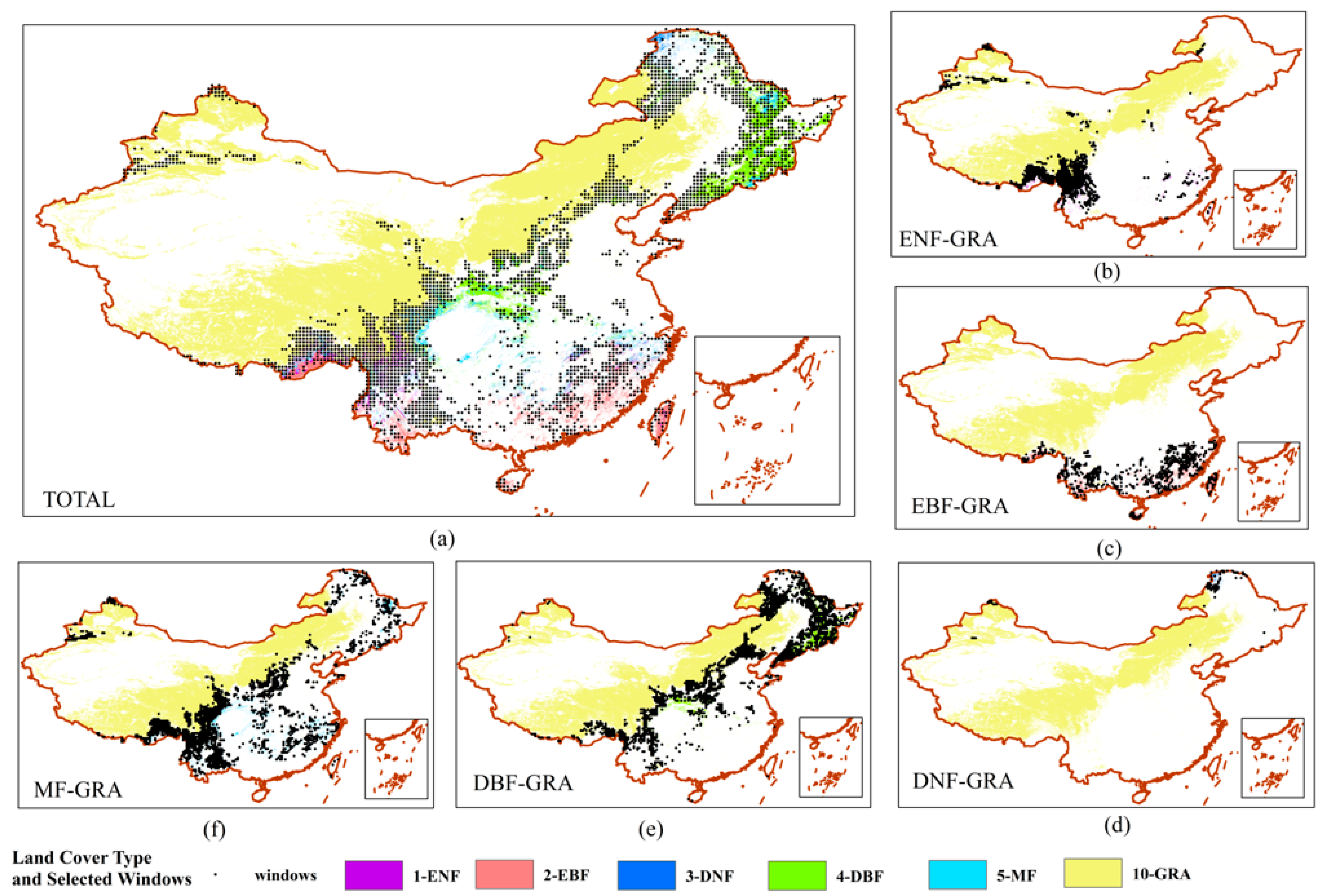
3.1. The Distribution of Potential Forest Conversion

We compared the spatial distribution of five potential forest conversions in this study with the optimized potential afforestation locations and tree species outlined in the latest published afforestation roadmap for China (refer to Figure 2c in [13]). Evergreen needleleaf forests (ENFs) were mainly located in Southwestern China and the Tianshan Mountains region in the northeast (Figure 1b), where the forestation roadmap recommended planting Picea-Abies, temperate Pinaceae, and warm Pinaceae. Evergreen broadleaf forests (EBFs) were distributed in Southern China (Figure 1c), where the forestation map suggested planting fast-growing evergreen and other evergreen broadleaf forests. Deciduous needleleaf forests (DNFs) were found in Northeastern China (Figure 1d), where the forestation roadmap recommended planting Larix spp. Deciduous broadleaf forests (DBFs) were broadly distributed from Northeastern to Southwestern China (Figure 1e), following the 400 mm annual precipitation contour. The forestation roadmap suggested the planting of Betula-Populus and other deciduous broadleaf forests. Mixed forests (MFs) were distributed in Southern, Southwestern, and Northeastern China, as well as the Tianshan Mountains region (Figure 1f), where temperate and subtropical mixed forests were shown to be suitable in the forestation roadmap.
The spatial distribution of potential forest conversions in our study aligns with the goals of the afforestation roadmap, which primarily emphasize the optimization of carbon sequestration. The observed consistency indicates that the biophysical climate effects (i.e., ΔLST) assessed in this study can indeed provide a more comprehensive evaluation of the climatic impacts of future afforestation.

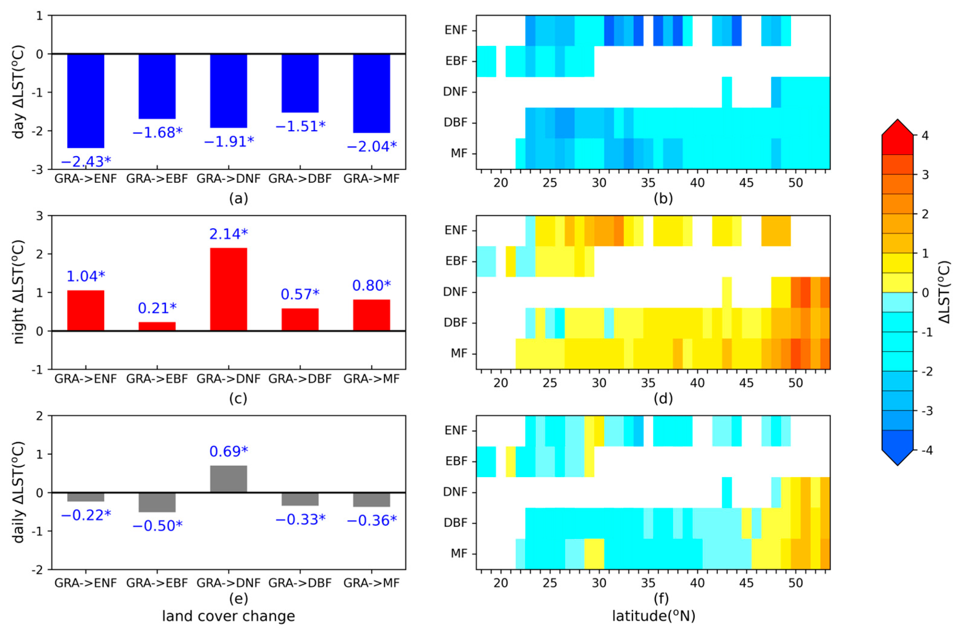
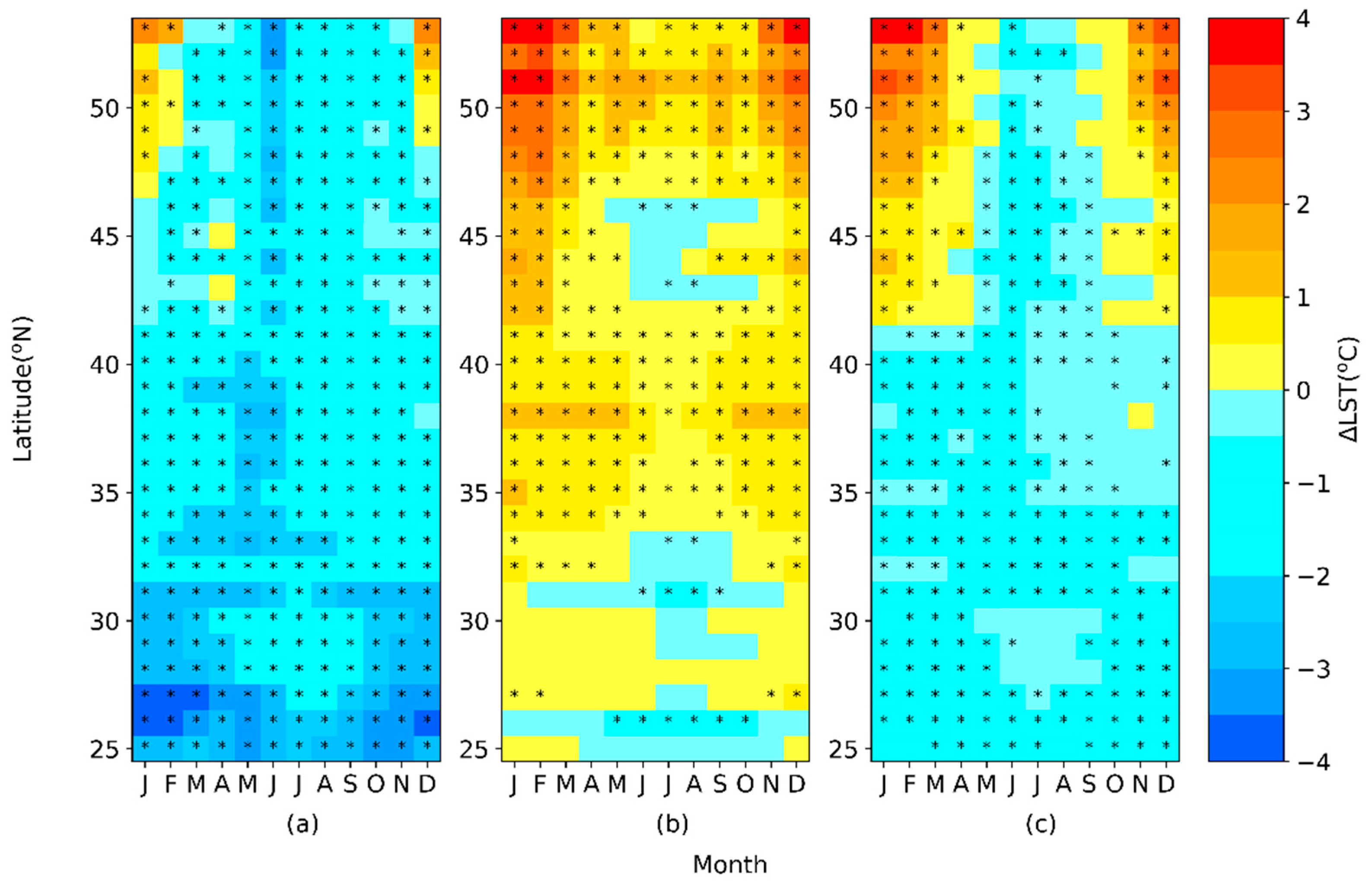
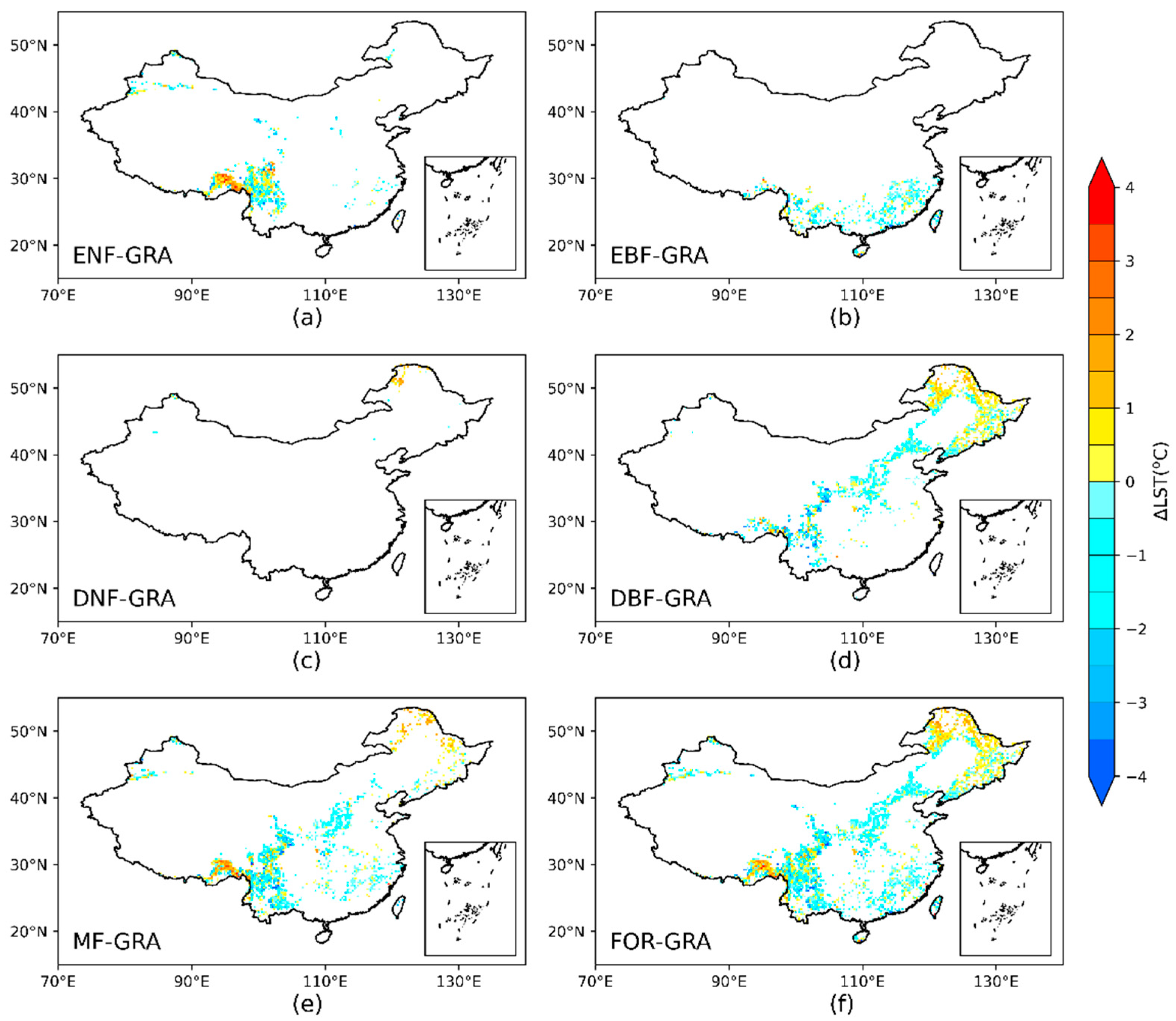
3.2. Potential Impact of Forest Conversion on ΔLST

Generally, afforestation had a daily cooling effect for all paired comparisons except for DNF. The net cooling effects of ENF, EBF, DBF, and MF were −0.22 ± 0.11 °C (mean ± 95% confidence interval, the same below), −0.50 ± 0.10 °C, −0.33 ± 0.05 °C, and −0.36 ± 0.06 °C, respectively. The daily cooling effect consisted of a large cooling effect during the day and a small warming effect at night (see Figure 2a,c). However, DNFs showed the opposite pattern, with daytime cooling surpassed by nighttime warming (Figure 2a,c, see GRA->DNF), resulting in a net warming of 0.69 ± 0.24 °C. These regionally averaged conclusions in mid-latitudes generally align with previous satellite-data-driven studies in terms of direction, but some differences in magnitude have been noted [9,11,17,25]. Until now, only limited studies have focused on the classification of sub-divided forests. Zhao et al. [14] have found that DBF expansion from grasslands lead to a regionally averaged LST decrease with the value of −0.11 ± 0.81 °C (mean ± SD) in North America. Meanwhile, ENF expansion induced cooling to a magnitude of −1.27 ± 1.6 °C (mean ± SD).
Our results suggested that the cooling effects of broadleaf forests were stronger than those of needleleaf forests, while Zhao et al. [14] showed the opposite. The reason for this discrepancy is still unclear, even though similar LST data and methodologies were used. Possible reasons could be the influence of significant spatial variations in sample distribution, the length of time series data utilized, and data quality control.
Combining Figure 1, Figure 2 and Figure 3, we further detected the relation between the distribution of paired vegetation cover types and their latitudinal patterns of ΔLST. Stable and adjacently distributed ENF and GRA were mainly concentrated in Southwestern China; they also occurred sporadically in the Xinjiang Province and Southeastern China (refer to Figure 1b). In the regional average, the ΔLST between ENF and GRA was negative; this means that the cooling effect during the day was stronger than the warming effect at night. On average, the comparison between ENF and GRA indicated a relatively weak cooling effect compared to the comparisons between broadleaf forests and grasslands (i.e., EBF vs. GRA, DBF vs. GRA), as well as between MF and GRA (see Figure 2e). The reasons for this are discussed in Section 4.
The comparison between EBF and GRA, as well as that between DNF and GRA, formed an interesting contrast: the former was distributed in Southern China (Figure 1c, below 30° N), while the latter was found in Northeastern China (Figure 1d, above 48° N). Correspondingly, EBF showed a significant cooling effect compared to GRA, while DNF exhibited a significant warming effect relative to GRA.
The distribution of DBF vs. GRA and MF vs. GRA spanned from the south to the north (Figure 1e,f), exhibiting similar and distinct patterns of latitudinal variation in ΔLST (Figure 3d,e). During the daytime, DBF (MF) showed a cooling effect compared to the surrounding GRA, but the magnitude of cooling decreased with the increasing latitude (see Figure 2b, DBF (MF)). At night, DBF (MF) had a higher LST than the neighboring GRA, and the magnitude of warming increased with the latitude (see Figure 2d, DBF (MF)). Daily ΔLST represented a transition from cooling to warming, with the transition zone occurring between 44 and 47° N (ΔLST = −0.02 ± 0.08 °C for DBF vs. GRA, and ΔLST = 0.11 ± 0.21 °C for MF vs. GRA). In addition, DBF and MF showed average daily cooling effects of −0.65 ± 0.07 °C and −0.48 ± 0.06 °C, r e s p e c t i v e l y , between 20 and 43° N, as well as average daily warming effects of 0.53 ± 0.08 °C and 0.81 ± 0.18 °C between 48 and 53° N.
Similar to previous findings, this study found that the biophysical climate impact of forestation on LST could be further translated into the latitudinal dependence of a warming effect in northern high latitudes and cooling effects in other latitudes, with the transitional latitude near 45–50° N [9,25]. These cooling or warming effects are mainly driven by the relative strength of the albedo-induced radiative warming and evapotranspiration (hereafter, ET)-dominated non-radiative cooling [4,7]. In this work, near boreal regions (>47° N), radiative warming surpassed non-radiative cooling, causing a positive LST signal. The radiative warming comes from the fact that forest canopies have a lower albedo due to their greater height, unevenness, and darker color compared to grasslands, resulting in the absorption of more solar shortwave radiation energy [21]. The monthly results further indicated that this positive LST signal mainly occurred from November to the following April (Figure 4c). This is because snow-covered short vegetation surfaces reflect more shortwave radiation energy back into Space [30]. For the remaining mid-latitude zones in this study, non-radiative cooling was found to counteract radiative warming, leading to an overall negative ΔLST. Tall, rough canopies like those in conifer forests exhibit strong ET and latent heat release when soil moisture is sufficient, resulting in a cooling effect [21]. This effect is most pronounced at lower latitudes but diminishes as the latitude increases due to soil moisture limitations [7,31]. The cooling effect primarily occurs during the daytime and depends on stomatal opening for transpiration [32,33]. Seasonally, non-radiative cooling showed larger magnitudes in the growing season than in the dormant season (Figure 4c).
The latitudinal pattern of ΔLST is also impacted by the seasonal variations. Figure 4 provided valuable insights into the intricate spatiotemporal ΔLST patterns. Given the extensive latitudinal distribution of DBF and GRA, they served as representative examples of these patterns. During the daytime, DBF generally exhibited a cooling effect, except for regions situated north of 47° N during the winter months (specifically, in December and January, as depicted in Figure 4a). Conversely, DBF predominantly displayed a warming effect at night, except for areas located south of 30° N and especially during the summer (as indicated in Figure 4b). The daily ΔLST revealed pronounced spatiotemporal heterogeneity. In regions positioned south of 41° N, ΔLST consistently showcased a cooling trend throughout the year. In regions north of 42° N, the prevailing pattern involved cooling during the summer and warming during the winter. Additionally, with increasing latitude, the duration and intensity of winter warming exhibited an upward trend. It is worth noting that the temperature effect in the range of 44–47° N was not significant and represented a transitional region. This could be attributed to the opposite diurnal and seasonal impacts that had similar magnitudes and hence canceled each other out on daily and annual scales (refer to Figure 4c). Interestingly, in regions south of 30° N, the spatiotemporal characteristics of daily ΔLST were mainly inherited from those of daytime ΔLST, mainly due to strong ET cooling of temperate forests. In regions north of 47° N, especially in winter when the ET cooling effect was weak, the spatiotemporal characteristics of daily ΔLST were mainly inherited from those of nighttime ΔLST; here, albedo-induced warming becomes notable.
Unlike the cooling effect of forests compared to grasslands at low latitudes, ENF and MF exhibited a warming region around 30° N (see Figure 3a,e, indicated in orange); the warming effect at night exceeded the cooling effect during the day (see Figure 2b,d,f, ENF and MF). We enlarged this region to examine the details, as shown in Figure 5a,b. The warming region was found to be mainly located in high-altitude mountainous areas (Figure 5c), and this was covered with snow in winter, as shown in Figure 5d. The dark forest canopies conceal the underlying snow-covered grassland surface and further lower surface albedo. Thus, the forest surface absorbs more energy, subsequently generating a local warming effect, like its behavior in high-latitude regions. These phenomena suggest that intricate local conditions, such as high altitudes, can cause local warming [34,35].
So far, we have found that afforestation in areas north of 48° N in China may lead to significant local warming. Therefore, caution should be exercised when planting DNFs, DBFs, and MFs in Northeast China. The southwestern region of China is home to a variety of tree species, making it suitable for large-scale afforestation. However, afforestation in mountainous areas may cause local warming, especially when planting ENFs and MFs. The mentioned tree species for planting refer to those that are ecologically adapted to the local environment. Furthermore, in regions that are suitable for diverse tree species planting, it is advisable to choose broadleaf and mixed forests for their enhanced local cooling impact.

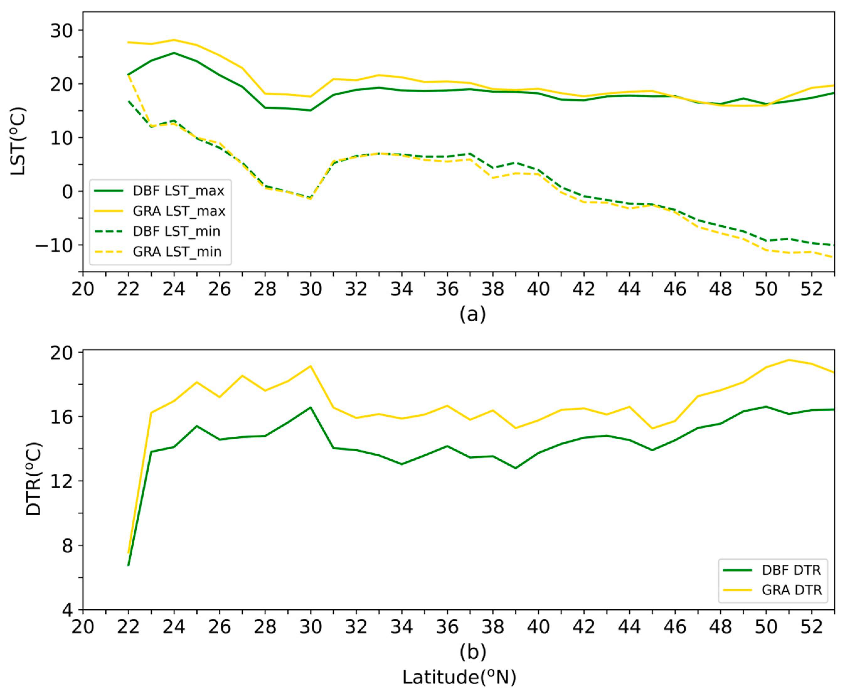
3.3. LST Patterns along Latitudinal Gradients: Perspective from DTR

The latitudinal pattern of diurnal temperature range (DTR) can also provide an alternative perspective on the differences in biophysical properties between forests and surrounding grasslands. DBFs had a smaller DTR than grasslands even at high latitudes (See Figure 6b), which implied that forests can provide a more moderate environment than short vegetations [30]. However, the origin of this reduced DTR varied at low and high latitudes. In regions below 38° N, DBFs had a diminished DTR primarily due to their lower daytime maximum LST compared to grasslands (refer to Figure 6a), which was attributed to higher ET and, correspondingly, more latent heat released at lower latitudes. In areas above 45° N, the smaller DTR in forests was primarily caused by their higher nighttime minimum LST compared to the adjacent grasslands (see Figure 6a). During the daytime, both forests and short vegetation experience water limitation in ET at high latitudes. However, the taller canopy heights of forests enable them to acquire more atmospheric energy through turbulent exchanges during the night, resulting in higher nighttime LST [36]. The perspective on DTR reinforces the impact of ET in shaping LST’s latitude-related changes.

4. Discussion

4.1. The Impact of Forest Types on Local Climate

Species differences in albedo and water and energy exchange can have effects that are important to the climate system. In ecosystems, the albedo values typically decrease from grasslands with standing dead leaves, which have high reflectivity, to broadleaf forests, and finally to dark coniferous forests [37]. The albedo is influenced not only by the reflectance of individual leaves, stems, and soil but also by the overall ecosystem structure. Complex canopies, due to interactions between leaves and stems, tend to have lower albedo compared to individual leaves, allowing for the efficient capture of light throughout the entire canopy. In contrast to broadleaf forests, coniferous forests have a more vertical angle of leaves in the upper canopy, reducing the likelihood of light saturation and enhancing the penetration of light through the canopy. So, coniferous forests are capable of thriving in high-latitude regions with less favorable lighting conditions (see Figure 1d). Additionally, the aggregation of needles around stems in coniferous forests facilitates the effective distribution of light within the canopy [21]. The literature indicates that evergreen needleleaf forests have an average surface albedo that is 0.02–0.03 lower than evergreen broadleaf forests, while deciduous needleleaf forests have an average surface albedo that is 0.00–0.01 lower than deciduous broadleaf forests [38,39]. Evergreen forests tend to be located in areas that are warm and wet, thus having a higher leaf area index and a lower surface albedo. On the other hand, canopies with shorter and smoother leaves, like grasslands, more effectively reflect incoming shortwave radiation from the upper leaves directly back to Space [20].
ET is another key factor that influences local climate and includes water vapor transpired by plants or evaporated from leaves or soil surfaces. In ecosystems, broadleaf forests have the highest ET values, followed by coniferous forests and then grasslands. Tall and uneven canopies are aerodynamically rough, allowing efficient energy and water vapor transfer away from the surface and mix in the atmosphere [30,40,41]. Conversely, air flow through short and smooth canopies, such as grasslands or crops, tends to have less turbulence, resulting in less overall interaction with the atmosphere. In general, energy flux from wet ecosystems is dominated by ET, whereas energy flux from other ecosystems, especially dry ones, is dominated by sensible heat flux [21]. For example, the transpiration rate in broadleaf forests is higher than in coniferous forests. Wilson et al. [42] measured Bowen ratios in different ecosystems during the summer, with values ranging from 0.25 to 0.5 in broadleaf forests and from 0.5 to 1 in coniferous forests. In this study, we found that evergreen broadleaf forests were mainly distributed in the humid southern regions of China (Figure 1c), where the release of a large amount of latent heat resulted in a lower ΔLST compared to the surrounding grasslands, with a value of −0.50 °C. In contrast, evergreen coniferous forests, primarily distributed in Southwestern China (Figure 1b), exhibited a relatively weak cooling effect compared to the comparisons between broadleaf forests and grasslands. The main difference may be attributed to the release of latent heat due to transpiration. While coniferous forests cannot cool the canopy surface through vigorous transpiration, their canopy structures have some features adapted to relatively cold and dry environments. Coniferous forests generally have stronger water interception and storage capabilities than broadleaf forests. The rough bark of coniferous trees can intercept up to 10% more precipitation than smooth-barked trees and shrubs [30,33]. Furthermore, coniferous forests have a deeper maximum root depth in mid-latitudes, allowing them to obtain more soil moisture [43].
Species characteristics influence the climate system through biophysical paths in terms of albedo and ET. Ma et al. [44] demonstrated that the spatiotemporal patterns of ΔLST were primarily determined by the net effect of ET-induced latent heat changes, followed by albedo-induced solar radiation absorption changes from the surface energy budget perspective. In the dominant northern coniferous forests, coniferous trees have lower albedo and stomatal conductance, thus transferring a large amount of sensible heat to the atmosphere, leading to local warming (Figure 1d). In contrast, broadleaf forests cause local cooling due to strong cooling from transpiration compared to grasslands (Figure 1c). Due to differences in distribution areas and canopy structure, it can be seen that the cooling effect of broadleaf forests, compared to grasslands, is generally stronger than that of coniferous forests.

4.2. Robustness of Potential Forest Change Impacts on LST

In our study, we did not strictly limit the number of pixels representing different vegetation types within each sample point; the only requirement was to have both forest and grassland pixels within a sample (see Table 1 for cases where pixel count equals to 1 and corresponding ΔLST values and numbers). This approach aimed to capture the latitude distribution effectively. The ΔLST resulting from potential forest cover change may not completely reflect the temperature variations that could occur when actual vegetation cover changes take place in the future [8,11]. This is due to the uncertain extent (e.g., deforestation often occurs in a scattered and partial manner) and duration (e.g., forests can be removed at different rates over multiple years) of the actual changes. However, potential changes will at least indicate the direction of local temperature changes when afforestation occurs in the future. Hence, we are additionally concerned about the robustness of the sample selection method in this study.
Earlier studies [8,9,45] have demonstrated that the choice of threshold for detecting forest cover change significantly affects the magnitude of the temperature impacts associated with forest changes. Table 1 shows the ΔLST values and sample numbers acquired through the selection of samples through the use of pixel thresholds varying from 1% to 5% (equivalent to 9–54 pixels). In the case of the ENF and GRA comparison, increasing the threshold led in a transition from cooling to warming effects for ENFs. This shift is primarily attributed to the fact that, with higher thresholds, the selected samples are predominantly located in low-latitude mountainous areas, subsequently behaving similarly to those in high-latitude regions. High altitude may disrupt latitudinal patterns, leading to differences in the magnitude and direction of ΔLST compared to regions at a similar latitude [34,35].
On the other hand, for the other four comparisons, increasing the threshold cannot alter the conclusion of whether forests exhibited warming or cooling effects. In the case of EBF and DNF comparisons, the increase in threshold rapidly reduced the sample numbers, indicating that the distributions of EBFs and DNFs were more dispersed compared to adjacent GRAs. For such dispersed paired comparisons, larger threshold values make it even less likely to detect stable change signals.

4.3. Implications and Future Work

Through an evaluation of the impact of five locally adapted forest types on the LST in China, this research enhances our comprehension of the intricate biophysical climate effects in the temperate region. Consequently, it contributes to a more comprehensive evaluation of China’s forestation roadmap, supporting the nation’s climate mitigation policies. Future work should quantify the overall impact of afforestation on local and regional climates through both biophysical and biogeochemical processes.

5. Conclusions

This study aims to understand how afforestation in China affects local and regional climates, focusing on five locally adapted forest types. By analyzing latitudinal patterns of ∆LST between five locally adapted forest types and adjacent grasslands using satellite-based observations, we made the following key findings: Firstly, broadleaf forests and mixed forests exhibit stronger cooling effects than coniferous forests, making them advisable choices for planting in regions that are suitable for diverse forest types. Secondly, temperate forests demonstrate a net cooling effect to the south of 43° N but a net warming effect to the north of 48° N compared to grasslands. We recommend caution when planting deciduous needleleaf forests, deciduous broadleaf forests, and mixed forests in Northeastern China, as there is potential for local warming to occur. Thirdly, in the mountainous areas of Southwestern China, especially when planting evergreen needleleaf forests and mixed forests, tree planting may lead to local warming. Overall, our study provides insights that complement China’s current afforestation roadmap, offering considerations beyond carbon sequestration benefits and supporting climate adaptation and mitigation policies.

Author Contributions

Conceptualization, W.M. and Y.W.; formal analysis, W.M. and Y.W.; funding acquisition, W.M.; methodology, W.M.; software, Y.W.; visuazation, W.M.; writing—original draft preparation, W.M.; writing—review and editing, Y.W. All authors have read and agreed to the published version of the manuscript.

Funding

This research was funded by National Natural Science Foundation of China, grant number 42005125.

Data Availability Statement

The data presented in this study are available on request from the corresponding author.

Acknowledgments

The author gratefully acknowledges Yue Wang for our inspiring discussions. The MODIS LST products MO(Y)D11A2 and Land cover products MCD12Q1 were retrieved through the online data pool of Level-1 and Atmosphere Archive & Distribution System Distributed Active Archive Center https://ladsweb.modaps.eosdis.nasa.gov/ (accessed on 10 January 2024).

Conflicts of Interest

The authors declare no conflicts of interest.

References

  1. Liu, Z.; Deng, Z.; He, G.; Wang, H.; Zhang, X.; Lin, J.; Qi, Y.; Liang, X. Challenges and Opportunities for Carbon Neutrality in China. Nat. Rev. Earth Environ. 2022, 3, 141–155. [Google Scholar] [CrossRef]
  2. Bonan, G.B. Forests and Climate Change: Forcings, Feedbacks, and the Climate Benefits of Forests. Science 2008, 320, 1444–1449. [Google Scholar] [CrossRef] [PubMed]
  3. Canadell, J.G.; Raupach, M.R. Managing Forests for Climate Change Mitigation. Science 2008, 320, 1456–1457. [Google Scholar] [CrossRef]
  4. Chen, C.; Park, T.; Wang, X.; Piao, S.; Xu, B.; Chaturvedi, R.K.; Fuchs, R.; Brovkin, V.; Ciais, P.; Fensholt, R.; et al. China and India Lead in Greening of the World through Land-Use Management. Nat. Sustain. 2019, 2, 122–129. [Google Scholar] [CrossRef]
  5. Yu, Z.; Ciais, P.; Piao, S.; Houghton, R.A.; Lu, C.; Tian, H.; Agathokleous, E.; Kattel, G.R.; Sitch, S.; Goll, D.; et al. Forest Expansion Dominates China’s Land Carbon Sink since 1980. Nat. Commun. 2022, 13, 5374. [Google Scholar] [CrossRef]
  6. National Development and Reform Commission; Ministry of Natural Resources of China. The Master Plan for Major Projects of National Important Ecosystem Protection and Restoration (2021–2035); National Development and Reform Commission and Ministry of Natural Resources of China: Beijing, China, 2020; pp. 10–11. Available online: https://www.ndrc.gov.cn/xxgk/zcfb/tz/202006/P020200611354032680531.pdf (accessed on 10 January 2024).
  7. Bright, R.M.; Davin, E.; O’Halloran, T.; Pongratz, J.; Zhao, K.; Cescatti, A. Local Temperature Response to Land Cover and Management Change Driven by Non-Radiative Processes. Nat. Clim. Chang. 2017, 7, 296–302. [Google Scholar] [CrossRef]
  8. Alkama, R.; Cescatti, A. Biophysical Climate Impacts of Recent Changes in Global Forest Cover. Science 2016, 351, 600–604. [Google Scholar] [CrossRef]
  9. Li, Y.; Zhao, M.; Motesharrei, S.; Mu, Q.; Kalnay, E.; Li, S. Local Cooling and Warming Effects of Forests Based on Satellite Observations. Nat. Commun. 2015, 6, 6603. [Google Scholar] [CrossRef]
  10. Alkama, R.; Forzieri, G.; Duveiller, G.; Grassi, G.; Liang, S.; Cescatti, A. Vegetation-Based Climate Mitigation in a Warmer and Greener World. Nat. Commun. 2022, 13, 606. [Google Scholar] [CrossRef]
  11. Li, Y.; De Noblet-Ducoudré, N.; Davin, E.L.; Motesharrei, S.; Zeng, N.; Li, S.; Kalnay, E. The Role of Spatial Scale and Background Climate in the Latitudinal Temperature Response to Deforestation. Earth Syst. Dynam. 2016, 7, 167–181. [Google Scholar] [CrossRef]
  12. Lee, X.; Goulden, M.L.; Hollinger, D.Y.; Barr, A.; Black, T.A.; Bohrer, G.; Bracho, R.; Drake, B.; Goldstein, A.; Gu, L.; et al. Observed Increase in Local Cooling Effect of Deforestation at Higher Latitudes. Nature 2011, 479, 384–387. [Google Scholar] [CrossRef] [PubMed]
  13. Xu, H.; Yue, C.; Zhang, Y.; Liu, D.; Piao, S. Forestation at the Right Time with the Right Species Can Generate Persistent Carbon Benefits in China. Proc. Natl. Acad. Sci. USA 2023, 120, e2304988120. [Google Scholar] [CrossRef] [PubMed]
  14. Zhao, K.; Jackson, R.B. Biophysical Forcings of Land-Use Changes from Potential Forestry Activities in North America. Ecol. Monogr. 2014, 84, 329–353. [Google Scholar] [CrossRef]
  15. Li, Y.; Zhao, M.; Mildrexler, D.J.; Motesharrei, S.; Mu, Q.; Kalnay, E.; Zhao, F.; Li, S.; Wang, K. Potential and Actual Impacts of Deforestation and Afforestation on Land Surface Temperature. J. Geophys. Res. Atmos. 2016, 121, 14372–14386. [Google Scholar] [CrossRef]
  16. Peng, S.-S.; Piao, S.; Zeng, Z.; Ciais, P.; Zhou, L.; Li, L.Z.X.; Myneni, R.B.; Yin, Y.; Zeng, H. Afforestation in China Cools Local Land Surface Temperature. Proc. Natl. Acad. Sci. USA 2014, 111, 2915–2919. [Google Scholar] [CrossRef]
  17. Duveiller, G.; Hooker, J.; Cescatti, A. The Mark of Vegetation Change on Earth’s Surface Energy Balance. Nat. Commun. 2018, 9, 679. [Google Scholar] [CrossRef]
  18. Lian, X.; Jeong, S.; Park, C.-E.; Xu, H.; Li, L.Z.X.; Wang, T.; Gentine, P.; Peñuelas, J.; Piao, S. Biophysical Impacts of Northern Vegetation Changes on Seasonal Warming Patterns. Nat. Commun. 2022, 13, 3925. [Google Scholar] [CrossRef]
  19. Yang, J.; Wu, Q.; Dakhil, M.A.; Halmy, M.W.A.; Bedair, H.; Fouad, M.S. Towards Forest Conservation Planning: How Temperature Fluctuations Determine the Potential Distribution and Extinction Risk of Cupressus funebris Conifer Trees in China. Forests 2023, 14, 2234. [Google Scholar] [CrossRef]
  20. Baldocchi, D.D.; Xu, L.; Kiang, N. How Plant Functional-Type, Weather, Seasonal Drought, and Soil Physical Properties Alter Water and Energy Fluxes of an Oak–Grass Savanna and an Annual Grassland. Agric. For. Meteorol. 2004, 123, 13–39. [Google Scholar] [CrossRef]
  21. Chapin, F.S., III; Matson, P.A.; Vitousek, P.M. Water and Energy Balance. In Principles of Terrestrial Ecosystem Ecology, 2nd ed.; Springer: New York, NY, USA, 2012; pp. 94–100. [Google Scholar]
  22. Mahmood, R.; Pielke, R.A.; Hubbard, K.G.; Niyogi, D.; Bonan, G.; Lawrence, P.; McNider, R.; McAlpine, C.; Etter, A.; Gameda, S.; et al. Impacts of Land Use/Land Cover Change on Climate and Future Research Priorities. Bull. Am. Meteorol. Soc. 2010, 91, 37–46. [Google Scholar] [CrossRef]
  23. Pielke, R.A., Sr.; Pitman, A.; Niyogi, D.; Mahmood, R.; McAlpine, C.; Hossain, F.; Goldewijk, K.K.; Nair, U.; Betts, R.; Fall, S.; et al. Land Use/Land Cover Changes and Climate: Modeling Analysis and Observational Evidence. WIREs Clim. Change 2011, 2, 828–850. [Google Scholar] [CrossRef]
  24. Chen, C.; Li, D.; Li, Y.; Piao, S.; Wang, X.; Huang, M.; Gentine, P.; Nemani, R.R.; Myneni, R.B. Biophysical Impacts of Earth Greening Largely Controlled by Aerodynamic Resistance. Sci. Adv. 2020, 6, eabb1981. [Google Scholar] [CrossRef]
  25. Li, Y.; Li, Z.-L.; Wu, H.; Zhou, C.; Liu, X.; Leng, P.; Yang, P.; Wu, W.; Tang, R.; Shang, G.-F.; et al. Biophysical Impacts of Earth Greening Can Substantially Mitigate Regional Land Surface Temperature Warming. Nat. Commun. 2023, 14, 121. [Google Scholar] [CrossRef] [PubMed]
  26. Sulla-Menashe, D.; Friedl, M. MODIS/Terra+Aqua Land Cover Type Yearly L3 Global 500m SIN Grid V061 [MCD12Q1]. NASA EOSDIS Land Processes Distributed Active Archive Center. 2020. Available online: https://lpdaac.usgs.gov/products/mcd12q1v061/ (accessed on 10 January 2024).
  27. Friedl, M.A.; Sulla-Menashe, D.; Tan, B.; Schneider, A.; Ramankutty, N.; Sibley, A.; Huang, X. MODIS Collection 5 Global Land Cover: Algorithm Refinements and Characterization of New Datasets. Remote Sens. Environ. 2010, 114, 168–182. [Google Scholar] [CrossRef]
  28. Wan, Z.M. MODIS/Terra(Aqua) Land Surface Temperature/Emissivity 8-Day L3 Global 500m SIN Grid V061 [MO(Y)D11A2]. NASA EOSDIS Land Processes Distributed Active Archive Center. 2019. Available online: https://lpdaac.usgs.gov/products/mod11a2v061/ (accessed on 10 January 2024).
  29. The Shuttle Radar Topography Mission (SRTM) Collection. SRTM Global 30 Arc Second Elevation [SRTMGL30v021]. NASA EOSDIS Land Processes Distributed Active Archive Center. 2019. Available online: https://lpdaac.usgs.gov/products/srtmgl30v021/ (accessed on 10 January 2024).
  30. Bonan, G.B. Surface Energy Fluxes. In Ecological Climatology: Principles and Applications, 2nd ed.; Cambridge University Press: Cambridge, UK, 2008; pp. 193–205. [Google Scholar]
  31. Shen, M.; Piao, S.; Jeong, S.-J.; Zhou, L.; Zeng, Z.; Ciais, P.; Chen, D.; Huang, M.; Jin, C.-S.; Li, L.Z.X.; et al. Evaporative Cooling over the Tibetan Plateau Induced by Vegetation Growth. Proc. Natl. Acad. Sci. USA 2015, 112, 9299–9304. [Google Scholar] [CrossRef] [PubMed]
  32. Huang, D.; Knyazikhin, Y.; Wang, W.; Deering, D.W.; Stenberg, P.; Shabanov, N.; Tan, B.; Myneni, R.B. Stochastic Transport Theory for Investigating the Three-Dimensional Canopy Structure from Space Measurements. Remote Sens. Environ. 2008, 112, 35–50. [Google Scholar] [CrossRef]
  33. Waring, R.H.; Running, S.W. Water Cycles. In Forest Ecosystems: Analysis at Multiple Scales, 3rd ed.; Academic Press: San Diego, CA, USA, 2007; pp. 50–52. [Google Scholar]
  34. Bellasio, R.; Maffeis, G.; Scire, J.S.; Longoni, M.G.; Bianconi, R.; Quaranta, N. Algorithms to Account for Topographic Shading Effects and Surface Temperature Dependence on Terrain Elevation in Diagnostic Meteorological Models. Bound. Layer Meteorol. 2005, 114, 595–614. [Google Scholar] [CrossRef]
  35. Chen, X.; Su, Z.; Ma, Y.; Yang, K.; Wang, B. Estimation of Surface Energy Fluxes under Complex Terrain of Mt. Qomolangma over the Tibetan Plateau. Hydrol. Earth Syst. Sci. 2013, 17, 1607–1618. [Google Scholar] [CrossRef]
  36. Zhang, M.; Lee, X.; Yu, G.; Han, S.; Wang, H.; Yan, J.; Zhang, Y.; Li, Y.; Ohta, T.; Hirano, T.; et al. Response of Surface Air Temperature to Small-Scale Land Clearing across Latitudes. Environ. Res. Lett. 2014, 9, 034002. [Google Scholar] [CrossRef]
  37. Essery, R. Large-Scale Simulations of Snow Albedo Masking by Forests. Geophys. Res. Lett. 2013, 40, 5521–5525. [Google Scholar] [CrossRef]
  38. Eugster, W.; Rouse, W.; Pielke, R.A., Sr.; McFadden, J.P.; Baldocchi, D.D.; Kittel, T.G.F.; Chapin, F.S.; Liston, G.E.; Vidale, P.L.; Vaganov, E.A.; et al. Land–Atmosphere Energy Exchange in Arctic Tundra and Boreal Forest: Available Data and Feedbacks to Climate. Glob. Chang. Biol. 2000, 6, 84–115. [Google Scholar] [CrossRef] [PubMed]
  39. Hollinger, D.Y.; Ollinger, S.V.; Richardson, A.D.; Meyers, T.P.; Dail, D.B.; Martin, M.E.; Scott, N.A.; Arkebauer, T.J.; Baldocchi, D.D.; Clark, K.L.; et al. Albedo Estimates for Land Surface Models and Support for a New Paradigm Based on Foliage Nitrogen Concentration. Glob. Chang. Biol. 2010, 16, 696–710. [Google Scholar] [CrossRef]
  40. Jarvis, P.G.; McNaughton, K.G. Stomatal Control of Transpiration: Scaling Up from Leaf to Region. In Advances in Ecological Research; MacFadyen, A., Ford, E.D., Eds.; Academic Press: Cambridge, MA, USA, 1986; Volume 15, pp. 1–49. [Google Scholar]
  41. Kelliher, F.M.; Jackson, R. The Physical Environment: A New Zealand Perspective. In Evaporation and the Water Balance; Sturman, A., Spronken-Smith, R., Eds.; Oxford University Press: Melbourne, Australia, 2001; pp. 206–217. [Google Scholar]
  42. Wilson, K.B.; Baldocchi, D.D.; Aubinet, M.; Berbigier, P.; Bernhofer, C.; Dolman, H.; Falge, E.; Field, C.; Goldstein, A.; Granier, A.; et al. Energy Partitioning between Latent and Sensible Heat Flux during the Warm Season at FLUXNET Sites. Water Resour. Res. 2002, 38, 30–31. [Google Scholar] [CrossRef]
  43. Canadell, J.; Jackson, R.B.; Ehleringer, J.B.; Mooney, H.A.; Sala, O.E.; Schulze, E.-D. Maximum Rooting Depth of Vegetation Types at the Global Scale. Oecologia 1996, 108, 583–595. [Google Scholar] [CrossRef]
  44. Ma, W.; Jia, G.; Zhang, A. Multiple Satellite-Based Analysis Reveals Complex Climate Effects of Temperate Forests and Related Energy Budget. J. Geophys. Res. Atmos. 2017, 122, 3806–3820. [Google Scholar] [CrossRef]
  45. Wickham, J.D.; Wade, T.G.; Riitters, K.H. Empirical Analysis of the Influence of Forest Extent on Annual and Seasonal Surface Temperatures for the Continental United States. Glob. Ecol. Biogeogr. 2013, 22, 620–629. [Google Scholar] [CrossRef]
Figure 1. The spatial distribution of vegetation cover (including five forest cover types and one grassland cover type) and selected sample windows. (a) Spatial distribution of all selected windows with all 6 vegetation types as background. (bf) Spatial distributions of sample windows for each paired comparison, with corresponding vegetation cover types as backgrounds. ENF(s)—evergreen needleleaf forest(s); EBF(s)—evergreen broadleaf forest(s); DNF(s)—deciduous needleleaf forest(s); DBF(s)—deciduous broadleaf forest(s); MF(s)—mixed forest(s); GRA(s)—grassland(s).
Forests 15 00182 g001
Figure 2. Potential surface temperature impacts of afforestation are calculated as the LST difference of forests minus nearby grasslands. The magnitude of ΔLST for each paired comparison in (a) daytime, (c) nighttime, and (e) daily. Here, for example, GRA->ENF means the change direction is from GRA to ENF (i.e., afforestation). The latitudinal pattern of ΔLST for each land cover type at 1° bands with insignifificant difference masked out by t test at 95% for (b) daytime, (d) nighttime, and (f) daily. The numbers marked with asterisks indicate that ΔLST is significant at 95% according to t-test. ENF(s)—evergreen needleleaf forest(s); EBF(s)—evergreen broadleaf forest(s); DNF(s)—deciduous needleleaf forest(s); DBF(s)—deciduous broadleaf forest(s); MF(s)—mixed forest(s); GRA(s)—grassland(s).
Forests 15 00182 g002
Figure 3. Spatial distribution of daily ΔLST for paired comparisons between (a) ENF and GRA, (b) EBF and GRA, (c) DNF and GRA, (d) DBF and GRA, and (e) MF and GRA. (f) The combined spatial distribution of the above five paired comparisons. ENF(s)—evergreen needleleaf forest(s); EBF(s)—evergreen broadleaf forest(s); DNF(s)—deciduous needleleaf forest(s); DBF(s)—deciduous broadleaf forest(s); MF(s)—mixed forest(s); GRA(s)—grassland(s).
Forests 15 00182 g003
Figure 4. Monthly means of latitudinal ΔLST between DBF and GRA in (a) daytime, (b) nighttime, and (c) daily. X-axes and Y-axes represent the month and the latitude, respectively. The grids marked with asterisks indicate that ΔLST is significant at 95% according to t-test. All the ΔLST results are obtained by averaging over period of 2001–2020. DBF(s)—deciduous broadleaf forest(s); GRA(s)—grassland(s).
Forests 15 00182 g004
Figure 5. Spatial distribution of daily ΔLST for paired comparisons between (a) ENF and GRA, (b) MF and GRA, (c) altitude and (d) snow water equivalent on 20 January 2010, at latitudes 27–33° N and longitudes 91–99° E. ENF(s)—evergreen needleleaf forest(s); MF(s)—mixed forest(s); GRA(s)—grassland(s).
Forests 15 00182 g005
Figure 6. (a) Latitudinal distribution of maximum and minimum LST and (b) the corresponding DTR for DBF and GRA. DBF(s)—deciduous broadleaf forest(s); GRA(s)—grassland(s); LST—land surface temperature; DTR—diurnal temperature range.
Forests 15 00182 g006
Table 1. The ΔLST values and sample numbers acquired through the selection of samples by using different pixel threshold. ENF(s)—evergreen needleleaf forest(s); EBF(s)—evergreen broadleaf forest(s); DNF(s)—deciduous needleleaf forest(s); DBF(s)—deciduous broadleaf forest(s); MF(s)—mixed forest(s); GRA(s)—grassland(s).
ΔLST (°C)
Type\Pixel191827364554
ENF vs. GRA−0.220.130.210.210.280.290.29
EBF vs. GRA−0.50−0.46−0.83−0.72−0.78−0.78
DNF vs. GRA0.690.620.671.38
DBF vs. GRA−0.33−0.47−0.60−0.63−0.54−0.49−0.50
MF vs. GRA−0.36−0.44−0.38−0.42−0.47−0.47−0.38
Selected Sample Numbers
Type191827364554
ENF vs. GRA69633624419015011185
EBF vs. GRA56335126220
DNF vs. GRA67531000
DBF vs. GRA16234812621811248562
MF vs. GRA1550519330224164126104
Disclaimer/Publisher’s Note: The statements, opinions and data contained in all publications are solely those of the individual author(s) and contributor(s) and not of MDPI and/or the editor(s). MDPI and/or the editor(s) disclaim responsibility for any injury to people or property resulting from any ideas, methods, instructions or products referred to in the content.

