Tracheids vs. Tree Rings as Proxies for Dendroclimatic Reconstruction at High Altitude: The Case of Pinus sibirica Du Tour

Abstract

Siberian pine (Pinus sibirica Du Tour) is a widespread and long-lived species in the northern hemisphere, which makes it a good potential proxy for climatic data. However, the tree-ring growth of this species weakly correlates with climatic conditions, which prevents its use in dendroclimatic reconstruction. It was proposed to use the measurements of tracheid characteristics as model predictors to reconstruct the smoothed temperature of the key periods in tree growth. In this study, algorithms for preprocessing tracheids and temperature data, as well as for model cross-validation, were developed to produce reliable high-resolution (weekly-based) temperature reconstructions. Due to the developed algorithms, the key time periods of Siberian pine growth were identified during the growing season—early June (most active cell development) and mid-July (setting new buds for the next growing season). For these time periods, reliable long-term temperature reconstructions (R² > 0.6, p < 10⁻⁸) were obtained over 1653–2018. The temperature reconstructions significantly correlated (p < 10⁻⁸) with independent reanalysis data for the 19th century. The developed approach, based on preprocessing tracheid and temperature data, shows new potential for Siberian pine in high-resolution climate reconstructions and can be applied to other tree species that weakly respond to climate forcing.

1. Introduction

Siberian pine forests are the most complex ecosystems in the Siberian taiga, characterized by regenerative-age dynamics, stability, spatial and temporal structure, and biodiversity [1]. The distribution range of Siberian pine (Pinus sibirica Du Tour), a forest-forming species of the “cedar” forest formation, extends from the northeast of European Russia to the south of East Siberia, reaching Mongolia in the southern part (http://agroatlas.ru/ru/content/related/Pinus_sibirica/map/, accessed on 27 June 2023).

The observed global warming of recent decades has contributed to a shift in the timespan of the active growing season and its heat availability [2,3,4]. The consequences of these changes are most acute at the edges of the growing range, where trees often grow at the limits of physiological endurance [5,6]. Moreover, the responses of tree plants to climate change are mixed, from range expansion to suppression or death [7,8,9,10,11]. Under current climate changes, it is therefore critical not only to understand the response of tree vegetation as an important part of the planetary carbon cycle [12,13,14,15] but also to obtain a quantitative assessment through robust reconstructions of long-term climatic fluctuations.

The use of long-term chronologies of the anatomical parameters of tree rings allows one to obtain a more accurate and detailed understanding of past and recent variability in principal climatic factors compared to simply analyzing tree-ring width (TRW) [16,17,18,19]. The seasonal development of xylem anatomical structure significantly determines tree productivity and survival; hence, forests’ vulnerability to climate change and their ability to fix carbon dioxide [20,21]. This approach also enhances opportunities to study the physiological mechanisms of plant adaptation to changing environmental conditions, due to changes in both hydraulic and mechanical functions of woody tissue [22,23,24]. Therefore, understanding how and at which intervals of the growing season the principal climatic factors (temperature or precipitation) modify the tree-ring structure turns out to be important both for reconstructing past climate-tree ring relationships and developing adequate prediction models of climatic factors influencing the anatomical structure of tree rings [24,25,26,27,28,29]. The application of the quantitative wood anatomy approach is particularly relevant for the species (i.e., Pinus sibirica Du Tour) for which the study of climate response is extremely difficult due to the limited climate sensitivity of their radial growth [30,31].

A unique 495-year chronology of wood anatomical characteristics for Siberian pine has recently been obtained for the timberline in the Western Sayan, which has made it possible to estimate the climatic response of tree-ring widths and integral anatomical characteristics (namely, TRW indices, mean and maximum radial cell diameters, and cell wall thickness) [19].

However, the dataset of detailed anatomical measurements used in this study, namely the radial cell diameter and cell wall thickness of Pinus Sibirica tracheidograms, allows us to estimate the century-old records of climate factors with much higher time resolution. In this work, we exploit the full potential of the anatomical structure of tree rings in a detailed analysis of their climatic response, with a focus on dendroclimatic reconstructions, using previously developed [32] and new approaches.

In this study, we employ tracheid measurements with the objective of revealing the potential of Pinus sibirica Du Tour for high-resolution temperature reconstructions. Algorithms for tracheid and temperature preprocessing and accurate model evaluation were developed. Additionally, two hypotheses were tested: (1) key periods of tree growth can be determined by the quality of the smoothed daily temperature reconstruction models, and (2) the use of TRW for modeling would not achieve the same reconstruction reliability as using tracheid data.

2. Materials and Methods

2.1. Climate Data

Temperature and precipitation data were obtained from the Tashtyp meteorological station (WMO 29956), 52.8 N, 89.9 E, 455 m a.s.l., and they included mean daily temperature and cumulative daily precipitation records from 1929 to 2016. Mean daily NOAA/CIRES/DOE 20th Century Reanalysis V3 temperatures were obtained from the Climate Explorer web platform (http://climexp.knmi.nl/select.cgi?field=c3t2m_daily, accessed on 29 August 2023), using the grid box region: longitude from 89.5 to 90.5 E, latitude from 52.5 to 53.5 N (Figure 1).

To create a dependent variable for the reconstruction from the raw temperature data, a two-way sequential smoothing algorithm was applied (Figure 2).

To suppress high-frequency fluctuations in the mean daily temperature, intra-annual smoothing with varying lengths $w$ of the sliding window (from 1 up to 14 days) was applied (Figure 2 and Figure S1). The optimal length of the sliding window was determined by optimization of the temperature reconstruction models as described below.

In addition to the intra-annual smoothing, an inter-annual smoothing procedure for temperature was applied to develop reconstruction models of the smoothed temperature based on anatomical characteristics. The second smoothing was done to reduce annual variance in temperature. We used a moving average with a sliding window of W years (from 1 to 11 years) (Figure 2 and Figure S2), using the same criteria to choose the length of W.

For each pair $\left(w, W\right)$ of intra- and inter-annual sliding windows, the set ${DOY}_{sig}\left(w, W\right)\subseteq \left\{152, \dots , 243\right\}$ was created as a subset of tree-ring growing days (DOYs, growing season). ${DOY}_{sig}\left(w, W\right)$ is the set of DOYs for which the Pearson correlation between inter-annual and intra-annual smoothed temperatures was highly significant (p < 0.001).

As a result of the two-way sequential smoothing algorithm, we obtained dependent variables $T_{inter}\left(w, W, doy\right)$ of inter-annual smoothed temperatures for the model.

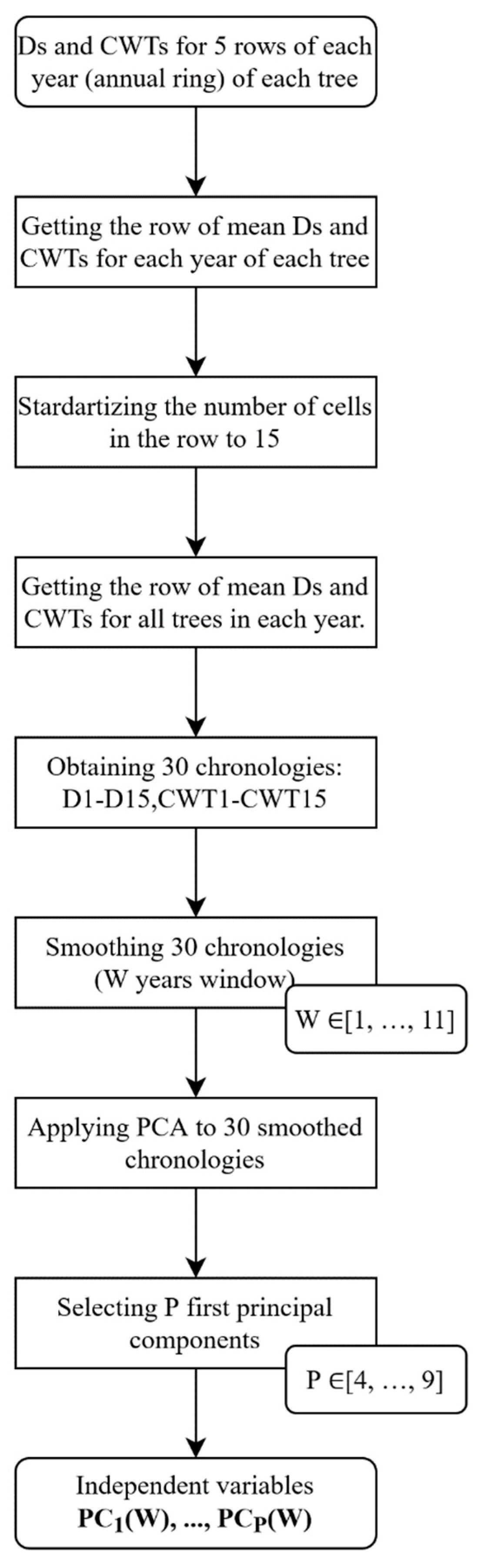
2.2. Tree Data Collection and Processing

Wood samples were collected from seven trees of Pinus sibirica Du Tour located on the border of the Republic of Khakassia and the Republic of Tyva (51°42.8′ N 89°51.9′ E, 1970–2020 m a.s.l.) (Figure 1). Tracheidogram measurements of tree rings over 1653–2018, obtained earlier (see [19] for more details), were used in this work (Figure S3).

For each tree ring, lumens (Ls) and double cell wall thickness (DCWT) were measured for 5 rows of cells (Figure S3). Then, the radial cell diameter (Cell Diameter, D) was calculated as the sum of lumen and double cell wall, and cell wall thickness (CWT) was determined as half of DCWT [33]. The obtained measurement were verified by an independent cell measuring tool [34].

The resulting tracheidograms of averaged D and CWT from the five rows of the measured series (Figure S4A,C) were then standardized to 15 cells (mean seasonal cell production over 1653–2018), resulting in standardized sD and sCWT series for each year of each tree [35]. Absolute tree ring width (TRW) values were obtained by summarizing DMeans of the corresponding rings.

The TRW values of all trees in a year were averaged to obtain the site tree-ring chronology. A standardized chronology was developed by bi-weight robust averaging individual tree indices, which were obtained by removing the age-related trends using cubic smoothing splines with a 50% frequency response at 67% of the series length [36].

The standardized tracheidograms of individual trees were year-to-year averaged (Figure S5). As a result, a single 30-dimensional object was obtained for each year (growing season), consisting of the values of cell diameters (D1–D15) and cell wall thicknesses (CWT1–CWT15) of the corresponding standardized curves (Figure S6).

Finally, 15 radial-cell-diameter and 15 cell-wall-thickness chronologies were obtained over 1653–2018 (Figure S7). Figure S8 shows examples of smoothed (“inter-seasonal smoothing”) chronologies of radial cell size and cell wall thickness. All the smoothed time series had significant Pearson correlations (p-value < 10⁻¹⁶) with D1–D15, CWT1–CWT15 series for all the sliding windows.

Principal component analysis (PCA) was applied to the radial-cell-size and cell-wall-thickness chronologies to reduce the dimensionality of the resulting 30-dimensional objects. It was shown that 4 principal components explained 95% of the variance of the series, while 9 principal components explained 99% of the variance (Figure S10). In addition, the application of PCA allows one to avoid multicollinearity in the obtained series, as noted above [37].

The first P principal components, smoothed with the inter-annual window W (see the example for P = 5, Figure S9):

$${PC}_i\left(W\right)=\left\{{pc}_i^W\left(y\right)|y\in \left\{1653\dots 2018\right\}\right\}, i\in \left[1, \dots , P\right]$$

(1)

were used as predictors (independent variables) in the model development process ($P\in [4,\dots ,9]$). The principal component transformation matrix is presented in Table S1.

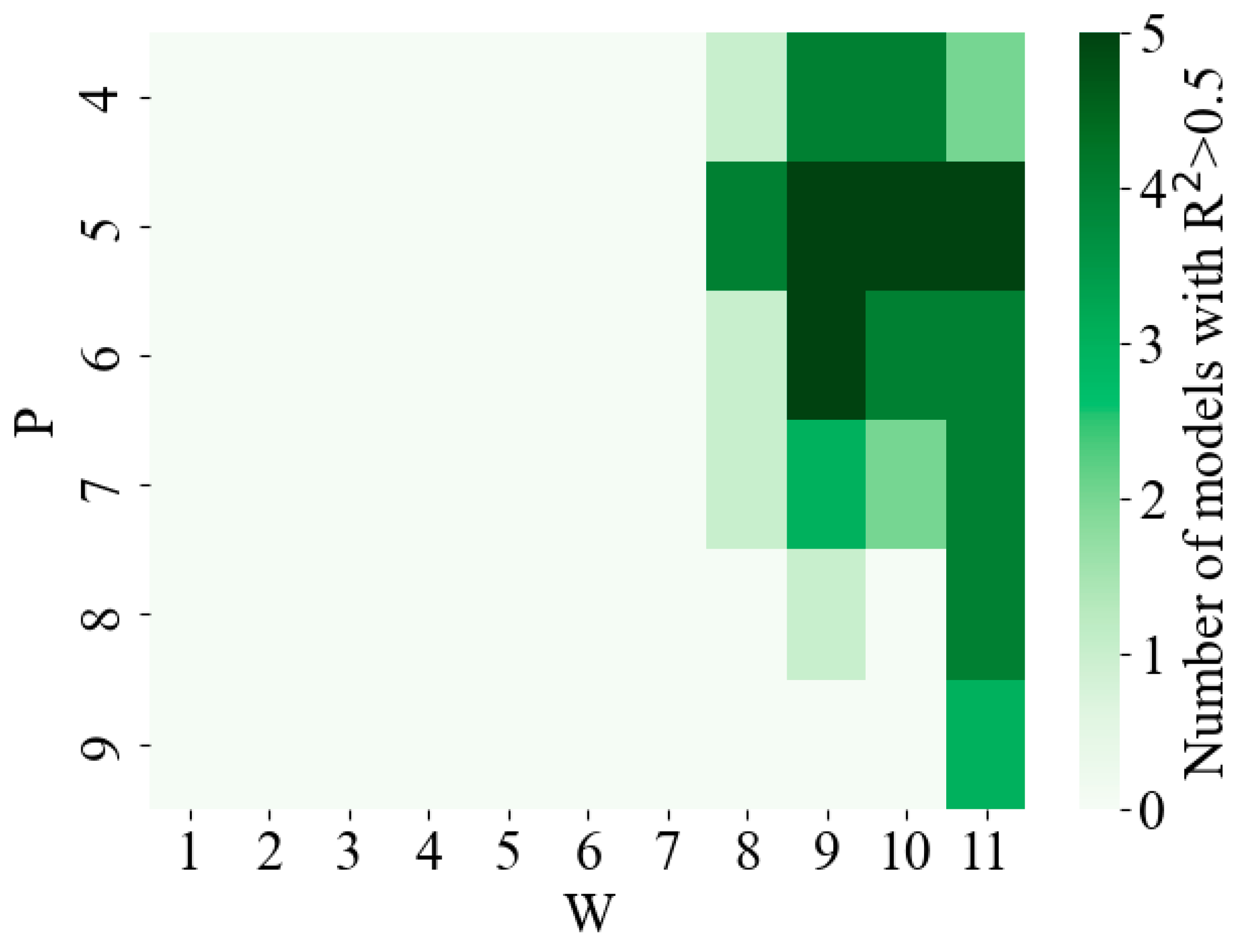
2.3. Reconstruction Models Development

For the best model fit, a triplet of hyperparameters $(w, W, P$) was varied as follows: $w\in \left\{1,\dots ,14\right\}, W\in \left\{1, \dots ,11\right\}, P\in \left\{4, \dots ,9\right\}$.

For each triplet $(w, W, P$), we obtained the set of independent variables $\{{PC}_1\left( W\right), \dots , {PC}_P\left( W\right)\}$(Figure 3) and the set of dependent variables $T_{inter}\left(w, W, doy\right), doy\in {DOY}_{sig}\left(w, W\right)$ (Figure 2).

For each $doy\in {DOY}_{sig}\left(w, W\right),$ a separate multiple linear regression (MLR) model ${MLR}_{w, W, P,doy} \left(year\right)$ was developed.

The final MLR models were considered as ensembles of individual MLR models obtained in a new rolling leave-one-out cross-validation (RLOO CV) procedure:

$${MLR}_{w, W, P,doy}\left(year\right)=k_0+{\sum }_{l=1}^P{k}_l· {pc}_i^W\left(y\right),$$

(2)

where $k_l=k_l\left(w,W,P,doy\right)$ is the $l$^th coefficient of the final MLR model ($l=\overline{0,P}$), estimated as $k_l=\frac{\sum _{\theta =1}^{N\left(W\right)}{k}_l^{\theta }}{N}$.

We note that $k_l^{\theta }=k_l^{\theta }\left(w, W, P,doy\right)$ is the $l$th coefficient of the $\theta$th individual MLR model, and $N=2016-1929+1=88$ is the total number of individual MLR models obtained in the RLOO CV procedure.

Each $\theta$th individual MLR model can be described by this formula:

$${MLR}_{w, W, P,doy}^{\theta }\left(year\right)=k_0^{\theta }+\sum _{l=1}^P{k}_l^{\theta }· {pc}_i^W\left(y\right), \theta =\overline{1929,2016}$$

(3)

To obtain the $\theta$th individual MLR model, $T_{inter}\left(w, W, doy\right)$ was split into calibration ($T_{inter}^{cal}\left(w, W, doy\right)$) and verification ($T_{inter}^{ver}\left(w, W, doy\right)$) sets by the rules of the RLOO CV procedure:

1.

Each $\theta$th element (year) of $T_{inter}\left(w, W, doy\right)$ is considered as a verification set.

2.

The elements from $\left[\theta -\left|\frac{W}{2}\right|,\theta \right)\cup \left(\theta ,\theta +\left|\frac{W}{2}\right|\right]$ are omitted ($\left|\frac{W}{2}\right|$ is the floored division).

This is done to prevent the data from the $\theta$th element from getting into the calibration set due to smoothing with the $W$ inter-annual sliding window and affecting the elements from $\left[\theta -\left|\frac{W}{2}\right|,\theta \right)\cup \left(\theta ,\theta +\left|\frac{W}{2}\right|\right]$.

All indices from $\theta -\left|\frac{W}{2}\right|<1929$ or $\theta +\left|\frac{W}{2}\right|>2016$ are ignored.

3.

All other elements are considered as a calibration set.

In this study, the RLOO CV procedure was developed as an extension of the LOO CV procedure [38] for smoothed data.

After obtaining the calibration and verification sets, the coefficients $k_l^{\theta }$ of the $\theta$th individual MLR model are obtained by training the model on the calibration set.

To evaluate the individual models on the calibration sets, the coefficient of determination ($R_{cal,\theta }^2$) and the Root Mean Squared Error (${RMSE}_{cal,\theta }$) were calculated between $T_{inter}^{cal}\left(w, W, doy\right)$ and $\left\{{MLR}_{w, W, P,doy}^{\theta }\left(year\right)|year\in T_{inter}^{cal}\left(w, W, doy\right)\right\}$.

After training the $N=88$ models, one for each year, the chronology of the verification values was obtained as:

$${CRN}_{w, W, P,doy}^{ver}=\left\{{MLR}_{w, W, P,doy}^{1929}\left(1929\right),\dots ,{MLR}_{w, W, P,doy}^{2016}\left(2016\right)\right\}$$

(4)

and the mean metrics $R_{cal}^2=\frac{\sum _{\theta =1929}^{2016}{R}_{cal,\theta }^2}{N}$, ${RMSE}_{cal}=\frac{\sum _{\theta =1929}^{2016}{RMSE}_{cal,\theta }}{N}$ were calculated to evaluate the total quality of the individual models on the calibration set.

To evaluate the individual models on the verification set, $R_{ver}^2$ and ${RMSE}_{ver}$ were calculated between ${CRN}_{w, W, P,doy}^{ver}$ and $T_{inter}\left(w, W, doy\right)$.

After individual evaluation, the final MLR model ${MLR}_{w, W, P,doy}\left(year\right)$ was developed by averaging the coefficients of the individual models.

To evaluate the final model, $R_{sim}^2$ and ${RMSE}_{sim}$ (sim—simulated) were calculated between $T_{inter}\left(w,W,doy\right)$ and $\left\{{MLR}_{w,W,P,doy}\left(year\right)|year\in T_{inter}\left(w,W,doy\right)\right\}$.

All data processing algorithms were implemented in Python and can be downloaded from: https://github.com/mikewellmeansme/dendroclimatic-reconstructor/ (accessed on 9 January 2024).

3. Results

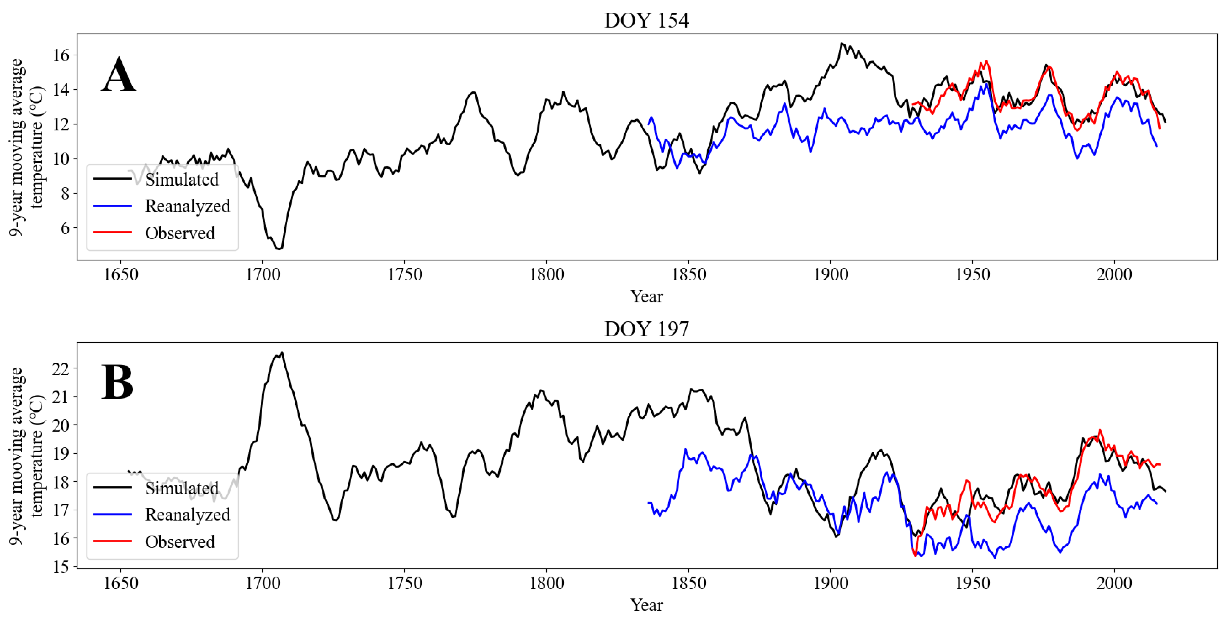
3.1. Reconstruction of Temperature Dynamics

We chose R² > 0.5 as a threshold for the selection of qualitatively reconstructed periods on the calibration and verification sets to be sure that the model explained most of the variance. After varying the triplet of hyperparameters $(w, W, P$), the next heatmap was obtained (Figure 4). Obviously, reliable reconstructions appeared when the annual smoothing windows W was not less than 8 years.

The approach of choosing the optimal triplet $(w, W, P)$ of hyperparameters is debatable, and different combinations of the triplet values sometimes result in the reconstruction of different days of the growth season. Mainly, temperatures at the beginning of June (weeks with DOY 152–154 at the center) and the middle of July (weeks with DOY 195-198 at the center) are adequately simulated by the tracheidograms.

There are also a couple of models for late June ($P=4$, DOY 175) and August (DOY 220 and 232), but these results are not sustainable because they do not appear with other triplets of hyperparameters.

As an example, we chose the triplet $w=7$, $W=9$, $P=5$ to demonstre the applicability of our approach to dendroclimatic reconstruction of summer temperatures (Figure 5).

We compared the new reconstructions with the observed and reanalyzed temperatures for two main sustainable periods: A—DOY 154 (the mean daily temperature from 30 May to 5 June) and B—DOY 197 (the mean temperature of the week from 12 July to 18 July) (Figure 6).

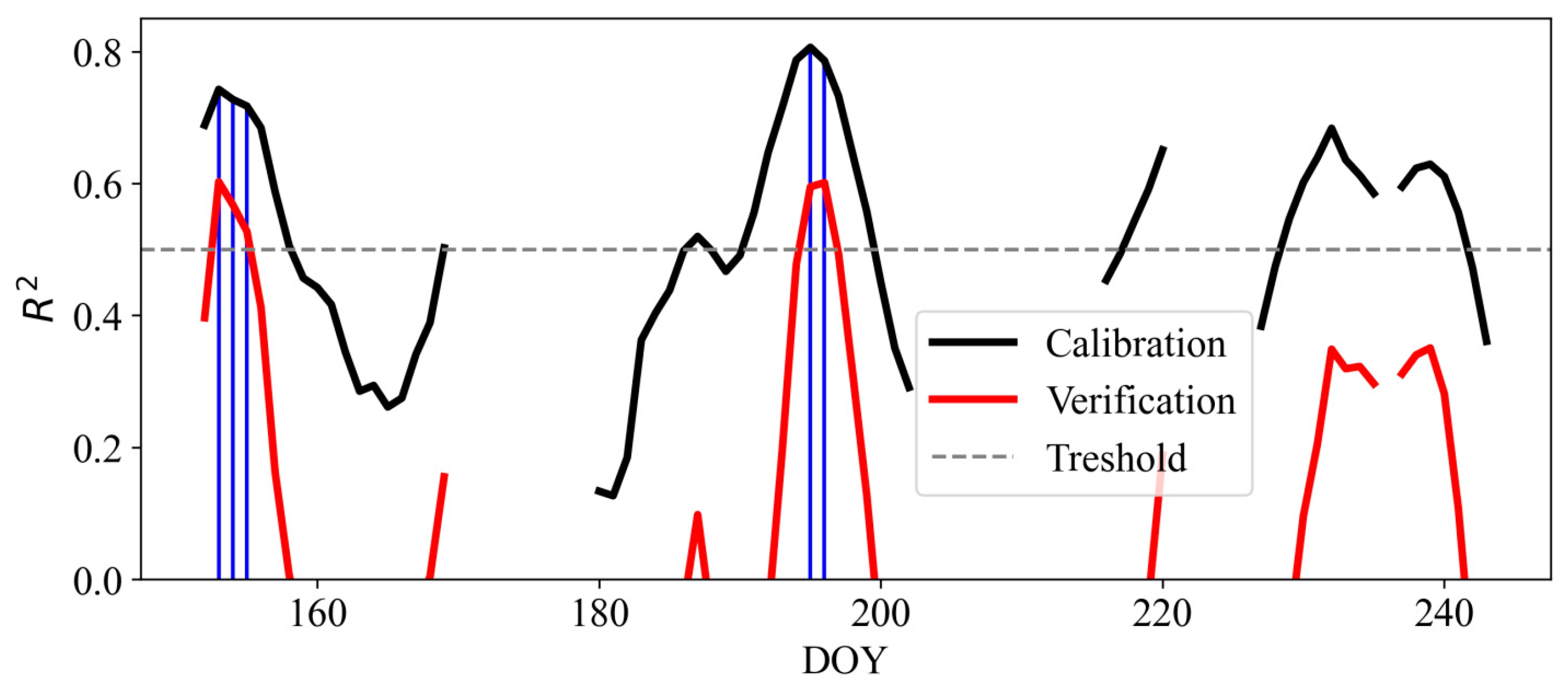
3.2. Reconstruction Model Evaluation

For each model, we obtained R² and RMSE metrics for the calibration set—performance of the models on the data on which they were trained; and for the verification set—performance of the models on the data that were not used in the training process. We also calculated simulated metrics—final performance of the models on the whole dataset. The obtained metrics are shown in

Table 1. Mean R² and RMSE obtained for the models during their calibration and verification.

Period	DOY	R2 Calibration	R2 Verification	R2 Simulated	RMSE Calibration	RMSE Verification	RMSE Simulated
A	154	0.74 ± 0.03	0.60	0.74	0.48 ± 0.15	0.60	0.48
B	197	0.79 ± 0.03	0.60	0.78	0.46 ± 0.15	0.63	0.46

.

Since different R² and RMSE were obtained for each iteration of the rolling cross-validation for the calibration set, Table 1 summarizes the mean values of the statistics on the calibration sample (±s.d.).

The obtained metrics show a reasonably high quality of the models, with more than 74% of the explained variance with RMSE less than 0.49 °C on the calibration set, and 60% of the explained variance with RMSE less than 0.63 °C on the verification set.

Figure 6 shows that, over the period of instrumental observations (1929–2016), the modeled (black line) and observed (red line) temperatures for both periods (A and B) have an extremely high degree of synchrony (R > 0.8, p < 10⁻²⁶,

Table 2. The Pearson correlations (Rs) and their significance (p) between the observed, reanalyzed, and simulated temperatures.

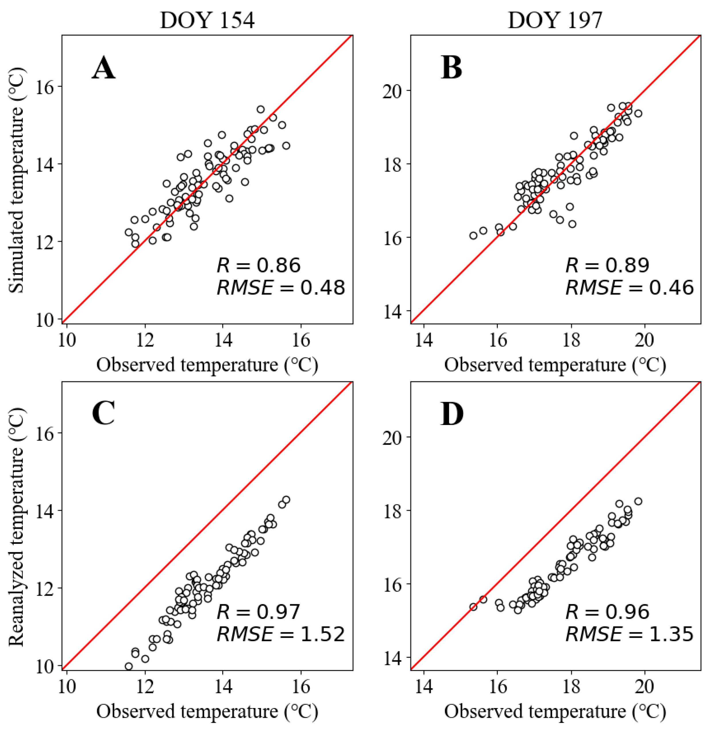
Years	Period	Observed\Reanalyzed		Observed\Simulated		Simulated\Reanalyzed
		Pearson R	p-Value	Pearson R	p-Value	Pearson R	p-Value
1836–1928	A	-	-	-	-	0.67	<10−12
	B	-	-	-	-	0.57	<10−8
1929–2016	A	0.97	<10−51	0.86	<10−26	0.79	<10−18
	B	0.96	<10−45	0.89	<10−29	0.81	<10−20

), as do the observed and reanalyzed temperatures (blue line) (R > 0.96, p < 10⁻⁴⁵, Table 2), but the reanalyzed data are significantly underestimated relative to the observed temperature (>1 °C) (see Figure 7 for more detail).

Due to their strong correlation with the observed temperature, despite the underestimation, the reanalyzed data can be taken as a reliable source of information on temperature trends. In this regard, the significant correlation (R > 0.56, p < 10⁻⁸, Table 2) between simulated and reanalyzed temperatures for the years with no direct climate observations (1836–1928) indicates that the models are sufficiently correct in indicating temperature trends for the modeled periods (A and B). In this paper, reanalyzed data are used for additional assessment of model quality beyond the metrics from Table 1.

The reanalyzed data are consistently underestimated (from 1.35 to 1.78 °C) relative to the observed data. This can be explained by the altitude difference between Tashtyp and the stations on the basis of which the reanalyzed data were constructed. As the altitude increases by 100 m, the temperature may proportionally decrease by a value close to 0.5 °C [39], so it can be assumed that the reanalyzed data are constructed on the basis of the data from the stations located 300–400 m above Tashtyp.

We noted that the obtained tree-ring width chronology did not correlate (p > 0.05) with the smoothed observed temperature of the Tashtyp weather station for intra-annual intervals up to 14-day smoothing.

Moreover, the enumeration of inter-annual sliding windows (Ws) for the standard TRW chronology from the range of 1 to 11 years did not allow one to obtain any models with R² > 0.5.

4. Discussion

It is known that both the width of tree rings and their anatomical structure are controlled by internal and external factors [35,40,41,42,43]. However, when comparing the variance and sensitivity coefficient of tree-ring width chronologies for different species under the same growing conditions, Siberian pine is shown to have rather low values of growth variability indices, even under climatically limited growing conditions [44,45]. There is no doubt that the low variability in Siberian pine growth is the result of a greater contribution of internal factors to its seasonal and perennial growth. These factors include adaptations of its physiology to the slow accumulation and utilization of nutrients [46,47], adaptations to wetter growing conditions (average variability of growth in other similar species of Siberian taiga, Siberian spruce, and Siberian fir [48,49]), and other ecophysiological features [50]. It is possible that the minor response of Siberian pine growth to low temperatures at high elevations is related to its genome size, which is larger than that in most tree species [51,52].

However, the long lifespan (up to 800–900 years [50,53]), wide distribution, and high economic and ecological value of Siberian pine have determined the ongoing attempts of dendrochronologists to obtain centuries-long annals of its tree rings and decode the contribution of the dynamics of environmental conditions, including climate forcing, on the formed rings. One of the approaches, due to a greater number of low-frequency fluctuations compared to annual fluctuations in tree-ring growth, is the use of smoothed time series with a window width of several years. The effectiveness of this approach was demonstrated in this work, and corresponds well with previously published results [30,54].

Another approach is to search more sensitive indicators of climate variability among the parameters of annual rings, including the use of quantitative wood anatomy. The use of long-term chronologies of tree-ring anatomical characteristics to reconstruct long-term changing climates over centuries is a relatively new and rapidly developing research direction [27,28,55,56].

We hypothesized that the ability to reconstruct seasonal, weekly-based temperature changes could be enhanced by using cell chronologies of Siberian pine anatomical characteristics, which was confirmed by both previously published results [19] and the new temperature reconstructions developed in the current research. Since the effects of internal factors are fairly uniform from year to year, by special treatment and combining the available cell measurements, we can accumulate the effects of external climate forcing and potentially reveal “hidden” correlations with climatic variables that cannot be observed based on traditional dendroclimatology techniques. To realize this approach, we developed several procedures to treat initial climate and anatomical data (Figure 2 and Figure 3). We also developed a new reconstruction procedure of seasonal temperatures (Figure 4) based on the principal component decomposition of cell measurements, specifically radial cell sizes and cell wall thickness.

The search for optimal windows for temperature generalization within a season and on a long-term scale allowed us not only to obtain reconstruction models that had high convergence with instrumental and reanalysis data but also established physiologically based regularities. The high first-order autocorrelation within a decade, accounting for the increased contribution of low-frequency oscillations and the possibility of preferential reconstruction of smoothed climatic series, can, at least partly, be attributed to the perennial needles of the species. It is known that needles of different species can persist for up to 14 years (e.g., spruce at the limit of distribution in the mountains; [57]). Siberian pine has a needle life span of 4–6 years at lower elevations and up to 9–10 years at higher elevations [58,59]. The age of needles of a related species, European cedar Pinus cembra, can reach 9–12 years [60,61].

The temperature intervals during the season, for which the reconstruction models showed the highest and most reliable statistical estimates, are important indicators of xylogenesis phenology. Thus, the first period in the first week of early June indicates the time interval of the most active growth of Siberian pine under certain local conditions, with sufficient humidity and increasing daylight but low heat availability. The second period (the week in the middle of July) corresponds to the interval of the end of primary growth and the budding for the development of shoots and needles for the next season [62,63,64].

The resulting models had quite high metrics. The metrics of the models based on tracheid data ($R>0.86$) are much higher than those of models based on tree ring widths ($R\in \left[0.2,0.6\right]$), both in the current work and compared to standard metric values of models based on climate-insensitive trees [19,65]. The obtained metric values are comparable to those from recent works on temperature reconstruction based on quantitative wooden anatomy of climate-insensitive species ($R^2>0.74$ on the calibration set) [65], which suggests that the cellular indices of these species are robust in explaining 60%–75% of the variance in temperature reconstruction.

In the current work, to test the quality of the models, in addition to the verification sample, whose data did not participate in the model training process and therefore can be considered independent, we also used V3 reanalysis grid data, with the modeled temperature also significantly correlating with these data, both during the years with instrumental measurements ($R>0.79$) and outside them ($R>0.57$).

Nevertheless, the potential of the proposed approach to modeling short-term climatic fluctuations requires further research. Various transformations or standardization of anatomical measurements may, for example, suppress a part of the non-climatic signal (including size-age) or the climatic signal inherited from previous stages of xylogenesis [66]. Different approaches to selecting relevant predictors among PCs and identifying promising intervals for intra- and inter-annual averaging, such as wavelet analysis, are worth exploring. The proposed approach can also be widely tested on new data from different forest stands with the same or other tree species that have low sensitivity to climate, as well as in different climatic zones.

5. Conclusions

The use of tracheid measurements has made it possible to realize the potential of Pinus sibirica Du Tour for high-resolution temperature reconstruction.

Using the developed algorithms, reliable models for temperature reconstruction were obtained. The seasonal, weekly-based intervals for which the models were obtained correlated with the key growth periods of Pinus sibirica Du Tour—the period of the highest cellular activity (early June) and the period of budding for the next season (mid-July), which confirmed our first hypothesis. Also, the smoothing windows, for which the first adequate reconstructions appeared, correlated with the lifespan of Pinus sibirica needles.

The use of tree ring widths as predictors did not allow one to obtain reliable reconstruction models for any seasonal time interval or with a single smoothing window due to their poor correlation with the temperature data. At the same time, the results of reconstructions derived from tracheid data did not only show good metric values for the verification set ($R^2>0.6$) but also had a significant correlation with the independent V3 reanalysis data for the 19th century ($p<{10}^{-8}$), which also confirmed the second hypothesis of this work.

Further modifying the developed algorithms can improve the quality of temperature reconstruction, but it is already evident at this stage that, despite the greater complexity of obtaining tracheidogram measurements compared to annual rings, quantitative wooden anatomy allows one to reconstruct temperature with much higher accuracy and resolution than classical approaches.

References

- Danchenko, A.M.; Beh, I.A. Cedar Forests of Western Siberia; Tomsk State University: Tomsk, Russia, 2010. [Google Scholar]
- White, A.; Cannell, M.G.R.; Friend, A.D. CO2 Stabilization, Climate Change and the Terrestrial Carbon Sink. Glob. Chang. Biol. 2000, 6, 817–833. [Google Scholar] [CrossRef]
- Menzel, A.; Sparks, T.H.; Estrella, N.; Koch, E.; Aaasa, A.; Ahas, R.; Alm-Kübler, K.; Bissolli, P.; Braslavská, O.; Briede, A.; et al. European Phenological Response to Climate Change Matches the Warming Pattern. Glob. Chang. Biol. 2006, 12, 1969–1976. [Google Scholar] [CrossRef]
- Huang, J.G.; Zhang, Y.; Wang, M.; Yu, X.; Deslauriers, A.; Fonti, P.; Liang, E.; Mäkinen, H.; Oberhuber, W.; Rathgeber, C.B.K.; et al. A Critical Thermal Transition Driving Spring Phenology of Northern Hemisphere Conifers. Glob. Chang. Biol. 2023, 29, 1606–1617. [Google Scholar] [CrossRef]
- Körner, C. Alpine Plant Life; Springer: Berlin/Heidelberg, Germany, 2003. [Google Scholar]
- Holtmeier, F.-K. Mountain Timberlines; Springer: Dordrecht, The Netherlands, 2009. [Google Scholar]
- Harsch, M.A.; Hulme, P.E.; McGlone, M.S.; Duncan, R.P. Are Treelines Advancing? A Global Meta-Analysis of Treeline Response to Climate Warming. Ecol. Lett. 2009, 12, 1040–1049. [Google Scholar] [CrossRef] [PubMed]
- Allen, C.D.; Macalady, A.K.; Chenchouni, H.; Bachelet, D.; McDowell, N.; Vennetier, M.; Kitzberger, T.; Rigling, A.; Breshears, D.D.; Hogg, E.H.; et al. A Global Overview of Drought and Heat-Induced Tree Mortality Reveals Emerging Climate Change Risks for Forests. For. Ecol. Manag. 2010, 259, 660–684. [Google Scholar] [CrossRef]
- Jochner, M.; Bugmann, H.; Nötzli, M.; Bigler, C. Tree Growth Responses to Changing Temperatures across Space and Time: A Fine-Scale Analysis at the Treeline in the Swiss Alps. Trees-Struct. Funct. 2018, 32, 645–660. [Google Scholar] [CrossRef]
- Lett, S.; Dorrepaal, E. Global Drivers of Tree Seedling Establishment at Alpine Treelines in a Changing Climate. Funct. Ecol. 2018, 32, 1666–1680. [Google Scholar] [CrossRef]
- McDowell, N.G.; Allen, C.D.; Anderson-Teixeira, K.; Aukema, B.H.; Bond-Lamberty, B.; Chini, L.; Clark, J.S.; Dietze, M.; Grossiord, C.; Hanbury-Brown, A.; et al. Pervasive Shifts in Forest Dynamics in a Changing World. Science 2020, 368, eaaz9463. [Google Scholar] [CrossRef]
- Lindner, M.; Maroschek, M.; Netherer, S.; Kremer, A.; Barbati, A.; Garcia-Gonzalo, J.; Seidl, R.; Delzon, S.; Corona, P.; Kolström, M.; et al. Climate Change Impacts, Adaptive Capacity, and Vulnerability of European Forest Ecosystems. For. Ecol. Manag. 2010, 259, 698–709. [Google Scholar] [CrossRef]
- Parks, C.G.; Bernier, P. Adaptation of Forests and Forest Management to Changing Climate with Emphasis on Forest Health: A Review of Science, Policies and Practices. For. Ecol. Manag. 2010, 259, 657–659. [Google Scholar] [CrossRef]
- Morin, X.; Fahse, L.; Jactel, H.; Scherer-Lorenzen, M.; García-Valdés, R.; Bugmann, H. Long-Term Response of Forest Productivity to Climate Change Is Mostly Driven by Change in Tree Species Composition. Sci. Rep. 2018, 8, 5627. [Google Scholar] [CrossRef]
- Pugh, T.A.M.; Lindeskog, M.; Smith, B.; Poulter, B.; Arneth, A.; Haverd, V.; Calle, L. Role of Forest Regrowth in Global Carbon Sink Dynamics. Proc. Natl. Acad. Sci. USA 2019, 116, 4382–4387. [Google Scholar] [CrossRef] [PubMed]
- Fonti, P.; Von Arx, G.; García-González, I.; Eilmann, B.; Sass-Klaassen, U.; Gärtner, H.; Eckstein, D. Studying Global Change through Investigation of the Plastic Responses of Xylem Anatomy in Tree Rings. New Phytol. 2010, 185, 42–53. [Google Scholar] [CrossRef] [PubMed]
- Wang, H.; Shao, X.; Fang, X.; Yin, Z.; Chen, L.; Zhao, D.; Wu, S. Responses of Pinus Koraiensis Tree Ring Cell Scale Parameters to Climate Elements in Changbai Mountains. Ying Yong Sheng Tai Xue Bao 2011, 22, 2643–2652. [Google Scholar]
- Wang, H.; Shao, X.; Fang, X.; Jiang, Y.; Liu, C.; Qiao, Q. Relationships between Tree-Ring Cell Features of Pinus Koraiensis and Climate Factors in the Changbai Mountains, Northeastern China. J. For. Res. 2017, 28, 105–114. [Google Scholar] [CrossRef]
- Zhirnova, D.F.; Belokopytova, L.V.; Upadhyay, K.K.; Tripathi, S.K.; Babushkina, E.A.; Vaganov, E.A. 495-Year Wood Anatomical Record of Siberian Stone Pine (Pinus Sibirica Du Tour) as Climatic Proxy on the Timberline. Forests 2022, 13, 247. [Google Scholar] [CrossRef]
- Anderegg, W.R.L. Spatial and Temporal Variation in Plant Hydraulic Traits and Their Relevance for Climate Change Impacts on Vegetation. New Phytol. 2015, 205, 1008–1014. [Google Scholar] [CrossRef]
- Sperry, J.S.; Love, D.M. What Plant Hydraulics Can Tell Us about Responses to Climate-Change Droughts. New Phytol. 2015, 207, 14–27. [Google Scholar] [CrossRef]
- Chave, J.; Coomes, D.; Jansen, S.; Lewis, S.L.; Swenson, N.G.; Zanne, A.E. Towards a Worldwide Wood Economics Spectrum. Ecol. Lett. 2009, 12, 351–366. [Google Scholar] [CrossRef]
- Von Arx, G.; Archer, S.R.; Hughes, M.K. Long-Term Functional Plasticity in Plant Hydraulic Architecture in Response to Supplemental Moisture. Ann. Bot. 2012, 109, 1091–1100. [Google Scholar] [CrossRef]
- Castagneri, D.; Fonti, P.; Von Arx, G.; Carrer, M. How Does Climate Influence Xylem Morphogenesis over the Growing Season? Insights from Long-Term Intra-Ring Anatomy in Picea Abies. Ann. Bot. 2017, 119, 1011–1020. [Google Scholar] [CrossRef] [PubMed]
- Tumajer, J.; Shishov, V.V.; Ilyin, V.A.; Camarero, J.J. Intra-Annual Growth Dynamics of Mediterranean Pines and Junipers Determines Their Climatic Adaptability. Agric. For. Meteorol. 2021, 311, 108685. [Google Scholar] [CrossRef]
- Tumajer, J.; Kašpar, J.; Kuželová, H.; Shishov, V.V.; Tychkov, I.I.; Popkova, M.I.; Vaganov, E.A.; Treml, V. Forward Modeling Reveals Multidecadal Trends in Cambial Kinetics and Phenology at Treeline. Front. Plant Sci. 2021, 12, 613643. [Google Scholar] [CrossRef] [PubMed]
- Pritzkow, C.; Wazny, T.; Heußner, K.U.; Słowiński, M.; Bieber, A.; Liñán, I.D.; Helle, G.; Heinrich, I. Minimum Winter Temperature Reconstruction from Average Earlywood Vessel Area of European Oak (Quercus Robur) in N-Poland. Palaeogeogr. Palaeoclimatol. Palaeoecol. 2016, 449, 520–530. [Google Scholar] [CrossRef]
- Ziaco, E.; Biondi, F.; Heinrich, I. Wood Cellular Dendroclimatology: Testing New Proxies in Great Basin Bristlecone Pine. Front. Plant Sci. 2016, 7, 223658. [Google Scholar] [CrossRef]
- Valeriano, C.; Gutiérrez, E.; Colangelo, M.; Gazol, A.; Sánchez-Salguero, R.; Tumajer, J.; Shishov, V.; Bonet, J.A.; Martínez de Aragón, J.; Ibáñez, R.; et al. Seasonal Precipitation and Continentality Drive Bimodal Growth in Mediterranean Forests. Dendrochronologia 2023, 78, 126057. [Google Scholar] [CrossRef]
- D’Arrigo, R.; Jacoby, G.; Frank, D.; Pederson, N.; Cook, E.; Buckley, B.; Nachin, B.; Mijiddorj, R.; Dugarjav, C. 1738 Years of Mongolian Temperature Variability Inferred from a Tree-Ring Width Chronology of Siberian Pine. Geophys. Res. Lett. 2001, 28, 543–546. [Google Scholar] [CrossRef]
- Cerrato, R.; Salvatore, M.C.; Gunnarson, B.E.; Linderholm, H.W.; Carturan, L.; Brunetti, M.; De Blasi, F.; Baroni, C. A Pinus cembra L. Tree-Ring Record for Late Spring to Late Summer Temperature in the Rhaetian Alps, Italy. Dendrochronologia 2019, 53, 22–31. [Google Scholar] [CrossRef]
- Zharkov, M.S.; Huang, J.G.; Yang, B.; Babushkina, E.A.; Belokopytova, L.V.; Vaganov, E.A.; Zhirnova, D.F.; Ilyin, V.A.; Popkova, M.I.; Shishov, V.V. Tracheidogram’s Classification as a New Potential Proxy in High-Resolution Dendroclimatic Reconstructions. Forests 2022, 13, 970. [Google Scholar] [CrossRef]
- Silkin, P.P. Methods of Multiparameter Analysis of Conifers Tree-Ring Structure; Siberian Federal University: Krasnoyarsk, Russia, 2010. [Google Scholar]
- Dyachuk, P.; Arzac, A.; Peresunko, P.; Videnin, S.; Ilyin, V.; Assaulianov, R.; Babushkina, E.A.; Zhirnova, D.; Belokopytova, L.; Vaganov, E.A.; et al. AutoCellRow (ACR)–A New Tool for the Automatic Quantification of Cell Radial Files in Conifer Images. Dendrochronologia 2020, 60, 125687. [Google Scholar] [CrossRef]
- Vaganov, E.A.; Hughes, M.K.; Shashkin, A.V. Growth Dynamics of Conifer Tree Rings; Springer: Berlin/Heidelberg, Germany, 2006. [Google Scholar]
- Cook, E.; Peters, K. The Smoothing Spline: A New Approach to Standardizing Forest Interior Tree-Ring Width Series for Dendroclimatic Studies. Tree-Ring Bull. 1981, 41, 45–53. [Google Scholar]
- Perez, L.V. Principal Component Analysis to Address Multicollinearity; Whitman College: Whitman, MA, USA, 2017. [Google Scholar]
- Hastie, T.; Tibshirani, R.; Friedman, J. The Elements of Statistical Learning; Springer Series in Statistics; Springer: New York, NY, USA, 2009; ISBN 978-0-387-84857-0. [Google Scholar]
- Chen, B.X.; Sun, Y.F.; Zhang, H.B.; Han, Z.H.; Wang, J.S.; Li, Y.K.; Yang, X.L. Temperature Change along Elevation and Its Effect on the Alpine Timberline Tree Growth in the Southeast of the Tibetan Plateau. Adv. Clim. Chang. Res. 2018, 9, 185–191. [Google Scholar] [CrossRef]
- Baas, P.; Wheeler, E.A. Wood Anatomy and Climate Change. Clim. Chang. Ecol. Syst. 2011, 78, 141–155. [Google Scholar] [CrossRef]
- Arzac, A.; Fonti, M.V.; Vaganov, E.A. An Overview on Dendrochronology and Quantitative Wood Anatomy Studies of Conifers in Southern Siberia (Russia). Prog. Bot. 2021, 83, 161–181. [Google Scholar] [CrossRef]
- Pandey, S. Climatic Influence on Tree Wood Anatomy: A Review. J. Wood Sci. 2021, 67, 24. [Google Scholar] [CrossRef]
- Anderson-Teixeira, K.J.; Herrmann, V.; Rollinson, C.R.; Gonzalez, B.; Gonzalez-Akre, E.B.; Pederson, N.; Alexander, M.R.; Allen, C.D.; Alfaro-Sánchez, R.; Awada, T.; et al. Joint Effects of Climate, Tree Size, and Year on Annual Tree Growth Derived from Tree-Ring Records of Ten Globally Distributed Forests. Glob. Chang. Biol. 2022, 28, 245–266. [Google Scholar] [CrossRef] [PubMed]
- Nazarov, A.N.; Myglan, V.S. Application of Siberian Cedar for Reconstruction of Climate and Geomorphological Events in Altai. Izv. Ross. Akad. Nauk. Seriya Geogr. 2015, 2, 43–51. [Google Scholar] [CrossRef]
- Shah, S.; Liu, Q.; Ahmad, A.; Mannan, A. Climate Growth Response of Pinus Sibirica (SIBERIAN PINE) in the Altai Mountains, Northwestern China. Pak. J. Bot. 2020, 52, 593–600. [Google Scholar] [CrossRef]
- Reich, P.B. The World-Wide ‘Fast–Slow’ Plant Economics Spectrum: A Traits Manifesto. J. Ecol. 2014, 102, 275–301. [Google Scholar] [CrossRef]
- Ning, Q.R.; Gong, X.W.; Li, M.Y.; Hao, G.Y. Differences in Growth Pattern and Response to Climate Warming between Larix Olgensis and Pinus Koraiensis in Northeast China Are Related to Their Distinctions in Xylem Hydraulics. Agric. For. Meteorol. 2022, 312, 108724. [Google Scholar] [CrossRef]
- Jiao, L.; Jiang, Y.; Wang, M.; Kang, X.; Zhang, W.; Zhang, L.; Zhao, S. Responses to Climate Change in Radial Growth of Picea Schrenkiana along Elevations of the Eastern Tianshan Mountains, Northwest China. Dendrochronologia 2016, 40, 117–127. [Google Scholar] [CrossRef]
- Lei, J.; Feng, X.; Shi, Z.; Bai, D.; Xiao, W. Climate–Growth Relationship Stability of Picea Crassifolia on an Elevation Gradient, Qilian Mountain, Northwest China. J. Mt. Sci. 2016, 13, 734–743. [Google Scholar] [CrossRef]
- Ignatenko, M.M. Siberian Cedar: (Biology, Introduction, Culture); Nauka: Moscow, Russia, 1988. [Google Scholar]
- MacGillivray, C.W.; Grime, J.P. Genome Size Predicts Frost Resistance in British Herbaceous Plants: Implications for Rates of Vegetation Response to Global Warming. Funct. Ecol. 1995, 9, 320. [Google Scholar] [CrossRef]
- Pellicer, J.; Leitch, I.J. The Plant DNA C-Values Database (Release 7.1): An Updated Online Repository of Plant Genome Size Data for Comparative Studies. New Phytol. 2020, 226, 301–305. [Google Scholar] [CrossRef] [PubMed]
- Nazarov, A.N.; Myglan, V.S. The Possibility of Construction of the 6000-Year Chronology for Siberian Pine in the Central Altai. J. Sib. Fed. Univ. Biol. 2012, 5, 70–88. [Google Scholar]
- Kharuk, V.I.; Ranson, K.J.; Im, S.T.; Dvinskaya, M.L. Response of Pinus Sibirica and Larix Sibirica to Climate Change in Southern Siberian Alpine Forest–Tundra Ecotone. Scand. J. For. Res. 2009, 24, 130–139. [Google Scholar] [CrossRef]
- González-Cásares, M.; Camarero, J.J.; Colangelo, M.; Rita, A.; Pompa-García, M. High Responsiveness of Wood Anatomy to Water Availability and Drought near the Equatorial Rear Edge of Douglas-Fir. Can. J. For. Res. 2019, 49, 1114–1123. [Google Scholar] [CrossRef]
- Seftigen, K.; Fuentes, M.; Ljungqvist, F.C.; Björklund, J. Using Blue Intensity from Drought-Sensitive Pinus Sylvestris in Fennoscandia to Improve Reconstruction of Past Hydroclimate Variability. Clim. Dyn. 2020, 55, 579–594. [Google Scholar] [CrossRef]
- Reich, P.B.; Oleksyn, J.; Modrzynski, J.; Tjoelker, M.G. Evidence That Longer Needle Retention of Spruce and Pine Populations at High Elevations and High Latitudes Is Largely a Phenotypic Response. Tree Physiol. 1996, 16, 643–647. [Google Scholar] [CrossRef]
- Sobchak, R.O.; Zotikova, A.P. Influence of High Altitude Conditions on Anatomo-Physiological Indices of Siberian Pine Needles. Bull. Tomsk. State Univ. 2009, 326, 200–202. [Google Scholar]
- Bender, O.G.; Zotikova, A.P.; Bender, A.G. The State of Photosynthetic Apparatus of Different-Aged Needles of Siberian Cedar at the Southern Limit of Growth in the Altai Mountains. In Proceedings of the Forest Biogeocenoses of the Boreal Zone: Geography, Structure, Functions, Dynamics, Krasnoyarsk, Russia, 16 September 2014; Sukachev Institute of Forest SB RAS, Federal Research Center “Krasnoyarsk Science Center SB RAS”: Krasnoyarsk, Russia, 2014; pp. 380–383. [Google Scholar]
- Günthardt, M.S.; Wanner, H. Die Menge des Cuticulären Wachses auf Nadeln von Pinus cembra L. und Picea abies (L.) Karsten in Abhängigkeit von Nadelalter und Standort. Flora 1982, 172, 125–137. [Google Scholar] [CrossRef]
- Nebel, B.; Matile, P. Longevity and Senescence of Needles in Pinus cembra L. Trees 1992, 6, 156–161. [Google Scholar] [CrossRef]
- Cooke, J.E.K.; Eriksson, M.E.; Junttila, O. The Dynamic Nature of Bud Dormancy in Trees: Environmental Control and Molecular Mechanisms. Plant Cell Environ. 2012, 35, 1707–1728. [Google Scholar] [CrossRef] [PubMed]
- Khare, S.; Drolet, G.; Sylvain, J.D.; Paré, M.C.; Rossi, S. Assessment of Spatio-Temporal Patterns of Black Spruce Bud Phenology across Quebec Based on MODIS-NDVI Time Series and Field Observations. Remote Sens. 2019, 11, 2745. [Google Scholar] [CrossRef]
- Silvestro, R.; Brasseur, S.; Klisz, M.; Mencuccini, M.; Rossi, S. Bioclimatic Distance and Performance of Apical Shoot Extension: Disentangling the Role of Growth Rate and Duration in Ecotypic Differentiation. For. Ecol. Manag. 2020, 477, 118483. [Google Scholar] [CrossRef]
- Lopez-Saez, J.; Corona, C.; von Arx, G.; Fonti, P.; Slamova, L.; Stoffel, M. Tree-Ring Anatomy of Pinus Cembra Trees Opens New Avenues for Climate Reconstructions in the European Alps. Sci. Total Environ. 2023, 855, 158605. [Google Scholar] [CrossRef]
- Meko, D.M.; Baisan, C.H. Pilot Study of Latewood-Width of Conifers as an Indicator of Variability of Summer Rainfall in the North American Monsoon Region. Int. J. Climatol. 2001, 21, 697–708. [Google Scholar] [CrossRef]