A Denoising Scheme for Scanned Wood Grain Images via Adaptive Color Substitution

Abstract

Real-world image denoising is a challenging problem in low-level vision. In order to reduce the luminance noise on scanned wood grain images randomly generated by the Microtek Phantom 9900XL scanner, the images were classified and sorted according to the noise size. The proposed denoising scheme reduces noise by substituting dissimilar pixels within a certain window size. The No.1 to No. 6 wood images with noise size of approximately (or no greater than) 3 pixels × 3 pixels were processed using coarse denoising with a 7 × 7 window ($\alpha$ = 100, $\beta$ = 30), fine denoising with a 5 × 5 window ($\alpha$ = 90, $\beta$ = 40), and the Dust & Scratches filter at settings of 1 (pixels) and 35 (levels). The No.7 to No. 16 wood images with noise size of approximately (or no greater than) 1 pixel × 1 pixel were processed using fine denoising with a 5 × 5 window ($\alpha$ = 100, $\beta$ = 30), and the Dust & Scratches filter at settings of 1 (pixel) and 35 (levels). The proposed Scheme I and II was then compared with Wiener filtering, Gaussian filtering, median filtering, and the Dust & Scratches filter under designated settings. The results of subjective and objective evaluations demonstrated that the proposed Scheme outperformed the above denoising methods on reducing the luminance noise. When using the median values of R (red), G (green), and B (blue) channels within a certain window to substitute the R, G, and B values of the luminance noise, the denoising ranges of $\alpha \ge 100$ and $\beta \le 30$ were suitable for the No.1 to No.16 wood images.

1. Introduction

Various visual characteristics of wood, which are broadly categorized into rich colors, varied textures, and mellow gloss, contribute to the unique appearance of wood. To imitate such excellent visual characteristics of natural wood grain, wood veneer [1] and decorative papers have been widely applied in the finishings of construction, panels, large furniture products, etc. These two surface decoration techniques, as well as the three-dimensional (3D) wood grain produced by ultraviolet (UV)-curable inkjet printing, are all realized based on two-dimensional (2D) images [2]. Thus, this paper will focus on the 2D digital wood grain that can be applied to the surface decoration of forest products. Unique from the research purposes of classification or recognition of wood species [3] and the detection of defects on wood surfaces [4], digital wood grain used for surface decoration is generally acquired in a static environment rather than a dynamic one.

Scanners and cameras are the commonly-used devices for the static image acquisition. In particular, flatbed scanners have the advantages of uniform illumination and freedom from stray light. The ability to recognize the nuances of color gradients is superior on charge-coupled device (CCD) scanners; color fidelity is greater and the range of colors is also wider [2]. As a result, the flatbed CCD scanner is often selected as the equipment for the digitization of color wood grain when it comes to the surface decoration with wood grain.

The optically scanned images captured using scanner sensors are often contaminated by noise (undesired random signal) [5,6,7]. The noise filter Dust & Scratches in Photoshop CC 2018 (Adobe Inc., San Jose, CA, USA) can reduce different types of noise by changing dissimilar pixels, and the balance between hiding defects and protecting image details can be achieved if it is controlled properly [8]. However, image details will be damaged to varying degrees when using the Dust & Scratches filter to reduce noise.

To solve this problem, Wen et al. [9] presented an efficient denoising method based on a Shearlet applied on the tree radar images, and proved that the proposed method had the best denoising performance in preserving the edge information. To promote structural smoothness and edge preservation in the image, Tan et al. [10] introduced a novel denoising method by combining the total variation (TV) regularization. To sum up, existing studies on image denoising methods are mostly aimed at reducing noise; meanwhile, enhancing or protecting image edges and textures.

Image denoising algorithms can be roughly divided into spatial-domain-based denoising, spatial-frequency-domain-based denoising, partial differential equations (PDE) denoising, the state-of-the-art algorithms such as C-BM3D (color version of block-matching and 3D filtering) [11], MC-WNNM (multi-channel weighted nuclear norm minimization) [12], TWSC (trilateral weighted sparse coding) [13], EPLL (expected patch log-likelihood) [14], etc., and so on.

The authors normally assume that the noise of distorted images is additive white Gaussian noise (AWGN) [15]. For example, Abdul Hamid et al. [16] proposed an image denoising module for wood images by using the expectation–maximization (EM) adaption algorithm, and the performance of the proposed module was compared to several classic denoising filters at various AWGN noise levels. The downside is that the EM adaption algorithm will become much less effective when dealing with the realistic noise captured by CCD cameras, because the realistic noise is much more complex than AWGN [13]. The testing of the effectiveness of these denoising algorithms on the publicly available real-world noisy image datasets is still demanded [17].

However, industrial wood images are different from the publicly available ones. Because of the disparate shooting or scanning conditions, the above-mentioned algorithms can still be invalid in the denoising of the scanned wood grain images even if the effectiveness of these algorithms on the publicly available image datasets has been tested. Moreover, for the images that will be applied to the large-scale production of decorative wood grain, these denoising algorithms in the literature are time-consuming and inefficient, since shorter processing time is crucial when dealing with large wood image databases [16].

In this paper, a denoising scheme for the scanned wood grain images via adaptive color substitution was proposed. It can be directly applied to realistic noise captured by CCD cameras. Weight matrices to characterize the statistics of realistic noise and the publicly available real-world wood image datasets are not necessary, which is of great convenience for wood grain image processing. Specifically, after analyzing the luminance noise on the scanned wood images randomly generated by the Microtek Phantom 9900XL scanner, the median values of R (red), G (green), and B (blue) channels within a certain window were used to substitute the R, G, and B values of the luminance noise that meet certain conditions, respectively. This denoising scheme is low in complexity, thereby, fast in computation, and especially suited to images that will be applied to large-scale production of decorative wood grain. Not only can it reduce the randomly generated noise on the scanned wood images effectively, but also preserve the texture details.

2. Materials and Methods

2.1. Source of Wood Images

The wood images for surface decoration were from 16 solid wood panels of different tree species. The surfaces of the solid wood panels were polished by waterproof abrasive 400-mesh paper and roller coated with waterborne transparent coatings. These clear and flat surfaces were then scanned by a CCD technology scanner (Phantom 9900XL, Microtek Co., Suzhou, China) with light-emitting diode (LED) light system, used according to reference [8].

One scanned plane was taken from each of the solid wood panels. Next, the 16 scanned planes were cropped to 120 mm × 900 mm (length × width), based on the size of the solid wood panels, and stored in a lossless TIFF format at 8 bits/channel and 300 pixels/inch resolution. Consequently, the image size of each scanned plane was 1417 pixels × 10,630 pixels with 256 gray levels.

Table 1. Basic information of the solid wood panels.

Panel Number	Tree Name	Scientific Name	Panel Size L (mm) × W (mm) × T (mm)
1	Intsia spp.	I. bijuga	150 × 1000 × 20
2	Tabebuia spp.	T. guayacan	150 × 1000 × 20
3	Robinia spp.	R. pseudoacacia	150 × 1000 × 20
4	Pometia spp.	P. pinnata	150 × 1000 × 20
5	Daniellia	D. klainei	150 × 1000 × 20
6	Pterocarpus spp.	P. soyauxii	150 × 1000 × 20
7	Piptadeniastrum	P. africanum	150 × 1000 × 20
8	Betula spp.	B. albosinensis	150 × 1000 × 20
9	Dalbergia	D. latifolia	150 × 1000 × 20
10	Quercus spp.	Q. rubra	150 × 1000 × 20
11	Carya spp.	C. illinoensis	150 × 1000 × 20
12	Swintonia spp.	S. pierrei	150 × 1000 × 20
13	Swietenia spp.	S. mahagoni	150 × 1000 × 20
14	Ulmus spp.	U. pumila	150 × 1000 × 20
15	Cylicodiscus	C. gabunensis	150 × 1000 × 20
16	Quercus spp.	Q. mongolica	150 × 1000 × 20

shows the basic information of the 16 solid wood panels. They have been classified and sorted by the following rules: No.1 to No.6 are the scanned planes with noise size of approximately (or no greater than) 3 pixels × 3 pixels, and No.7 to No.16 have noise size of approximately (or no greater than) 1 pixel × 1 pixel.

Table 2. The local parts of the scanned wood grain images from No.1 to No.16.

No.1	No.2	No.3	No.4	No.5	No.6
No.7	No.8	No.9	No.10	No.11	No.12
No.13	No.14	No.15	No.16

The image size shown above has been enlarged to 36 times the original size, which is 30 mm × 30 mm.

shows the local parts of the scanned planes from No.1 to No.16, and the size of each local image is 59 pixels × 59 pixels (5 mm × 5 mm). The various sensor noises were categorized as either color noise or luminance noise [18]. It is obvious from Table 2 that the noise randomly generated by the Microtek Phantom 9900XL scanner is luminance noise.

2.2. Adpative Color Substitution

2.2.1. Noise Analysis

Table 3. Mean, maximum, and minimum values of R, G, and B channels of the wood grain images from No.1 to No.16.

Image Number	Mean Values			Maximum Values			Minimum Values
	${\mathit{\mu }}_{\mathit{R}}$	${\mathit{\mu }}_{\mathit{G}}$	${\mathit{\mu }}_{\mathit{B}}$	${\mathit{I}}_{\mathit{R}\_\mathit{m}\mathit{a}\mathit{x}}$	${\mathit{I}}_{\mathit{G}\_\mathit{m}\mathit{a}\mathit{x}}$	${\mathit{I}}_{\mathit{B}\_\mathit{m}\mathit{a}\mathit{x}}$	${\mathit{I}}_{\mathit{R}\_\mathit{m}\mathit{i}\mathit{n}}$	${\mathit{I}}_{\mathit{G}\_\mathit{m}\mathit{i}\mathit{n}}$	${\mathit{I}}_{\mathit{B}\_\mathit{m}\mathit{i}\mathit{n}}$
1	119.31	63.11	11.68	251	201	224	0	0	0
2	118.61	71.63	16.85	210	202	192	0	0	0
3	126.13	83.57	34.14	253	230	214	0	0	0
4	153.27	84.31	50.29	255	222	204	0	0	0
5	147.08	79.89	21.93	244	214	205	7	0	0
6	138.97	90.54	41.40	237	205	203	0	0	0
7	173.92	113.61	67.54	255	233	236	0	0	0
8	193.48	140.76	87.53	255	233	204	37	10	0
9	188.87	120.74	80.77	255	223	203	34	0	0
10	188.38	129.59	81.98	255	224	212	59	0	0
11	191.11	141.17	98.74	253	226	208	8	23	0
12	180.38	133.53	102.04	255	255	238	21	0	0
13	190.15	117.48	54.18	255	237	187	0	0	0
14	166.74	114.33	67.67	254	225	209	0	0	0
15	149.00	78.15	12.23	255	214	188	0	0	0
16	169.87	120.44	76.02	248	226	208	0	0	0

shows the mean, maximum, and minimum values of R, G, and B channels of the wood grain images from No.1 to No.16.

Table 4. R, G, and B values of three luminance noise points on the wood grain images.

Image Number	Noise I			Noise II			Noise III
	R Values	G Values	B Values	R Values	G Values	B Values	R Values	G Values	B Values
1	135	137	161	102	122	141	130	137	154
2	173	152	147	120	118	160	133	115	127
3	168	149	152	145	107	133	129	132	123
4	167	158	157	162	140	160	192	179	189
5	193	176	183	178	157	172	196	184	179
6	166	158	164	196	180	173	175	171	183

shows the R, G, and B values of some random noise on these images.

From Table 3, the differences among the means of R, G, and B are significant; while from Table 4, the R, G, and B values of the random noise are quite close and relatively large, which is consistent with the characteristics of the luminance noise [18].

In summary, the R, G, and B values of the luminance noise to be replaced should meet the following conditions:

• $\mathrm{R}>\alpha$, $\mathrm{G}>\alpha$, and $\mathrm{B}>\alpha$;
• $\left|\mathrm{R}-\mathrm{B}\right|<\beta$, $\left|\mathrm{R}-\mathrm{G}\right|<\beta$, and $\left|\mathrm{G}-\mathrm{B}\right|<\beta$,

where $\alpha$ and $\beta$ are the constants.

Based on the color values of the wood grain images in Table 3 and the pixel values of the luminance noise in Table 4, $\alpha \ge 100$ and $\beta \le 30$ are suggested. As $\alpha$ values decrease and $\beta$ values increase, the probability of detecting the noise is higher.

As can be seen from Table 3, the maximum values of R, G, and B channels are mostly approaching to 255, and the minimum values of the three channels are mostly zero. Therefore, the median values of R, G, and B channels within a certain window were used to substitute the R, G, and B values of the luminance noise, respectively.

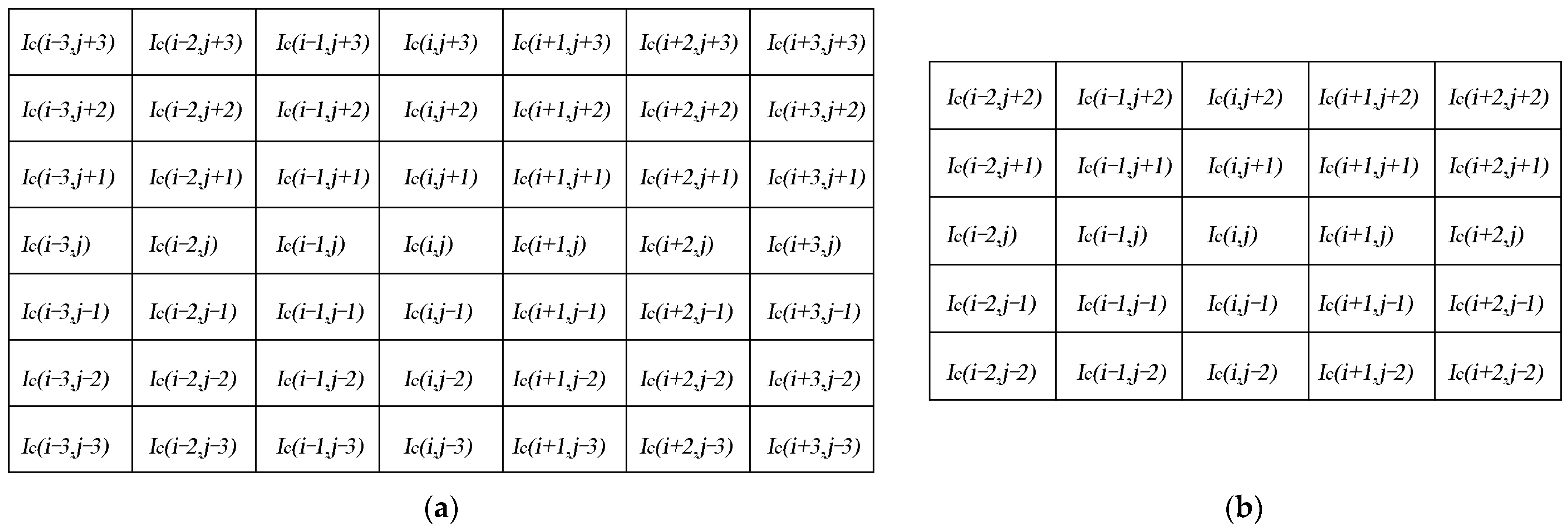
2.2.2. Noise-Searching Window

Texture details will be easier to lose and computation speed will be slower when the noise-searching window is large.

For the scanned planes from No.1 to No.6 with noise size of approximately (or no greater than) 3 pixels × 3 pixels, if the window size is set to 5 × 5, the median values within the window are more likely to be the noise pixels. Thus, the noise-searching window for the No.1 to No.6 scanned planes was set to 7 × 7.

The 7 × 7 window is shown in Figure 1a, where $c\in \left\{\mathrm{R},\mathrm{G},\mathrm{B}\right\}$, $I_c(i,j)$ is the pixel value of one point at the image coordinate.

Accordingly, for the scanned planes from No.7 to No.16 with noise size of approximately (or no greater than) 1 pixel × 1 pixel, the window size was set to 5 × 5 (Figure 1b), where $c\in \left\{\mathrm{R},\mathrm{G},\mathrm{B}\right\}$, $I_c(i,j)$ is the pixel value of one point at the image coordinate.

2.2.3. Algorithm Flow

For the scanned planes from No.1 to No.6 with visible noise, the $\alpha$ value was set to 100 and the $\beta$ value was set to 30 when performing coarse denoising with the 7 × 7 window.

Notably, when performing fine denoising with the 5 × 5 window in the next step, the α value should be less than 100, and the β value should be more than 30, otherwise the luminance noise cannot be detected. Using this method, the image will not be changed in any way. For this reason, the $\alpha$ value was reset to 90 and the $\beta$ value was reset to 40 when performing the fine denoising.

Since only fine denoising with the 5 × 5 window was to be performed on the scanned planes from No.7 to No.16 with visually unapparent noise, the $\alpha$ value was set to 100 and the $\beta$ value was set to 30 directly.

Figure 2 presents the algorithm flow chart, which is divided into three steps: (1) Decomposition of the source image, $I$; (2) Conditional judgment of the pixel values of R, G, and B channels within a certain window: if $\mathrm{R}>\alpha$, $\mathrm{G}>\alpha$, $\mathrm{B}>\alpha$, $\left|\mathrm{R}-\mathrm{B}\right|<\beta$, $\left|\mathrm{R}-\mathrm{G}\right|<\beta$, and $\left|\mathrm{G}-\mathrm{B}\right|<\beta$, the pixel at a certain point is considered as a noise pixel, and it should be substituted by the median values of R, G, and B channels within the window, respectively; otherwise the pixel at this point remains unchanged; (3) Merging the output R, G, and B channels to obtain the processed image, $I_{out}$.

Because the substituted colors on the processed images could not be naturally fused with the surrounding colors, the noise filter Dust & Scratches at settings of 1 (pixels) and 35 (levels) was used after the above procedures, and the texture details of the non-light-colored wood grain images could be well-preserved at this setting [8].

2.3. Image Quality Assessment

2.3.1. Subjective Observation

Two-scale decomposition was performed on the denoised images for better observation. It separates each source image into a base layer containing the large-scale variations in intensity and a detail layer containing the small-scale details by average filtering [19]. The base layer and detail layer of each source image are obtained as follows:

$$B_c=I_c\times Z$$

(1)

and

$$D_c=I_c-B_c,$$

(2)

where $c\in \left\{\mathrm{R},\mathrm{G},\mathrm{B}\right\}$, $I_c$ is the source image, $B_c$ is the base layer, $D_c$ is the detail layer, and $Z$ is the average filter.

The size of the average filter was set to 1417 × 1417 as the image size of each scanned plane was 1417 pixels × 10,630 pixels. By selecting this large-size average filtering, the image details are fully extracted [20], thus, making it easier to observe the noise and the denoising effect of wood grain images.

The realistic noise varies among the different channels. As the noise is typically strongest in the blue channel [18], and denoising mainly works on this channel [21]; thus, the detail layer of the blue channel was chosen to exhibit the denoising effect.

2.3.2. Objective Evaluation

The widely-used no-reference image quality assessment (NR-IQA) metrics include the blind image quality index (BIQI) [22], blind/referenceless image spatial quality evaluator (BRISQUE) [23], Natural Image Quality Evaluator (NIQE) [24], Distortion Identification-based Image Verity and Integrity Evaluation (DIIVINE) [25], and so on.

Deviations from the statistical regularities observed in natural images (NI), i.e., the regularity of the natural scene statistic (NSS), enable these space domain algorithms with the capability of assessing the perceptual quality of an image without the need for any reference image [26] or the training on human-rated distorted images [24].

Since the scanned images are natural images [27], two of the NR-IQA metrics BRISQUE and NIQE were chosen to evaluate the quality of the denoised images. The lower these two values are, the better the images are perceived by the human eyes.

3. Results and Discussion

Two types of linear filters, Wiener filtering and Gaussian filtering, the non-linear median filtering, and the noise filter Dust & Scratches at settings of 1 (pixels) and 35 (levels) were compared to the proposed denoising algorithm.

All the experiments were implemented in MATLAB R2018b on a PC with an Intel (R) Core (TM) i7-8550U CPU, 8 GB RAM.

3.1. Denoising of the No.1 to No.6 Wood Images

As the noise size on the No.1 to No.6 wood images was approximately (or no greater than) 3 pixels × 3 pixels, the window size of the Wiener filtering, Gaussian filtering, and median filtering was set to 5 × 5. The window size of the Gaussian filtering is theoretically [6 × sigma − 1]/2 × 2 + 1 ([ ] represents taking an integer), so the standard deviation, $\sigma$, should be set to 5/6. If $\sigma$ is large, the filtering effect improves, but the images become fuzzy [27]. For better denoising effect of the wood images, the $\sigma$ was unified set to 1 in this paper. The proposed denoising Scheme I to be conducted on these images was divided into three steps:

• Coarse denoising with the 7 × 7 window, where $\alpha$ = 100, $\beta$= 30;
• Fine denoising with the 5 × 5 window, where $\alpha$= 90, $\beta$= 40;
• Photoshop denoising using its Dust & Scratches filter at settings of 1 (pixels) and 35 (levels).

3.1.1. Evaluation of Visual Effect

Table 5. Denoising effect of the No.1 to No.6 wood images under different denoising methods.

Tree Name	Index	Wiener filtering (5 × 5)	Gaussian filtering (5 × 5)	Median filtering (5 × 5)	Dust & Scratches Filter	Proposed Scheme I	Original Images
No.1 Intsia spp.	RGB 1
	$D_B$ 2
No.2 Tabebuia spp.	RGB
	$D_B$
No.3 Robinia spp.	RGB
	$D_B$
No.4 Pometia spp.	RGB
	$D_B$
No.5 Daniellia	RGB
	$D_B$
No.6 Pterocarpus spp.	RGB
	$D_B$

¹ RGB represents the RGB color images; ² $D_B$ represents the detail layer of the blue channel; The image size shown above has been enlarged to 4.84 times the original size, which is 22 mm × 22 mm.

displays the local parts of the No.1 to No.6 wood images and their detail layers of the blue channels under different denoising methods. The size of each local image is 118 pixels × 118 pixels (10 mm × 10 mm).

From Table 5, the noise on the No.1 to No.6 wood images denoised using median filtering almost disappeared, but these images were the most vague. The images denoised using Wiener filtering and Gaussian filtering also exhibited ambiguity in varying degrees.

The images denoised using the Dust & Scratches filter at settings of 1 (pixels) and 35 (levels) and the proposed denoising Scheme I retained more texture details, but in terms of denoising effect, the proposed Scheme I was better.

As the evaluation of visual effects could be influenced by subjective consciousness, an objective evaluation was implemented to further illustrate the denoising effect of different methods adopted in wood image processing.

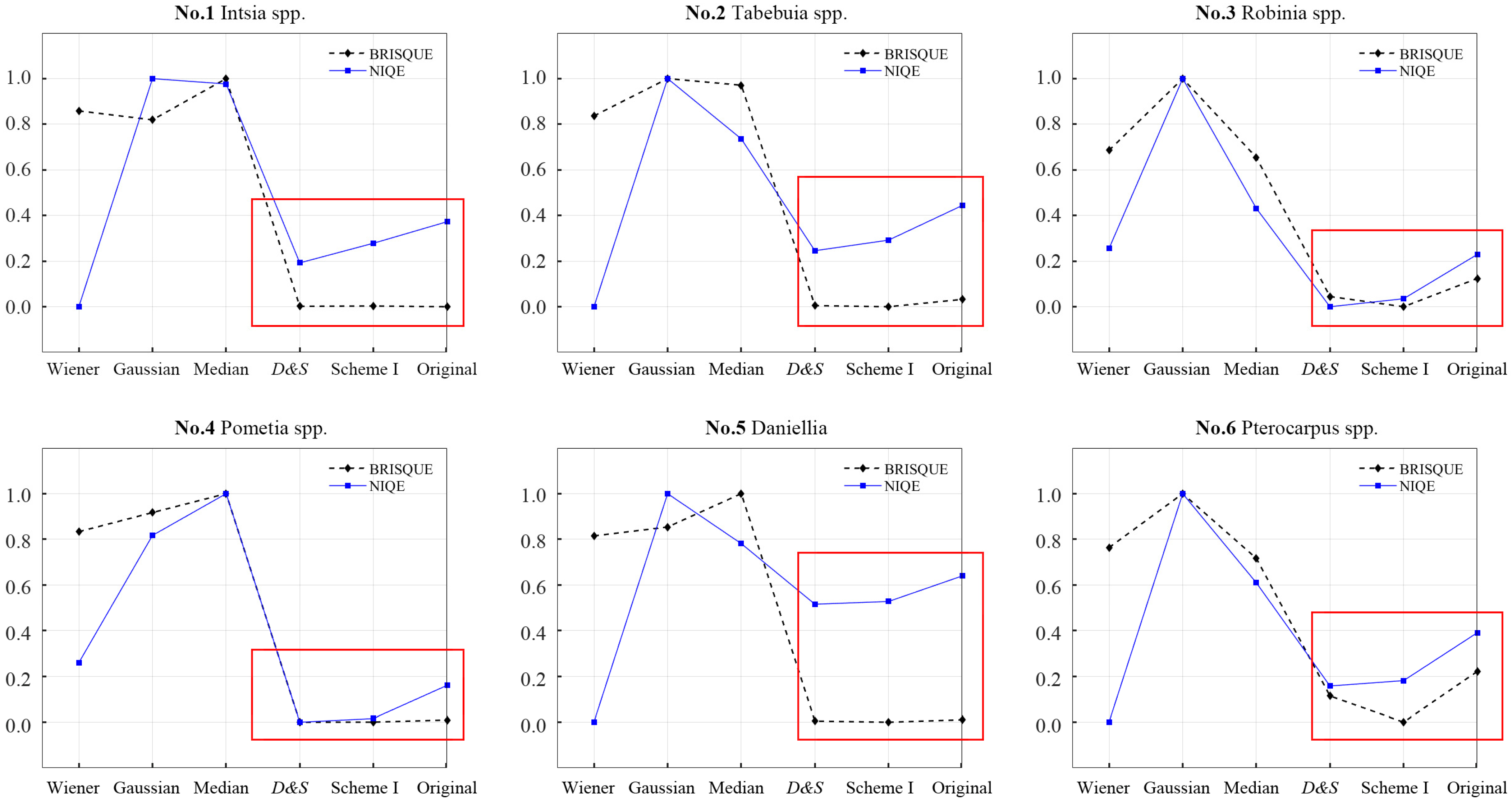
3.1.2. Evaluation of BRISQUE and NIQE

The evaluation values of BRISQUE and NIQE of the No.1 to No.6 wood images under different denoising methods are shown in

Table 6. IQA results of the No.1 to No.6 wood images under different denoising methods.

Image Number	Wiener Filtering (5 × 5)		Gaussian Filtering (5 × 5)		Median Filtering (5 × 5)		Dust & Scratches Filter		Proposed Scheme I		Original Images
	B 1	N 2	B	N	B	N	B	N	B	N	B	N
1	41.20	5.01	39.46	6.20	47.49	6.17	3.16	5.24	3.22	5.34	3.08	5.45
2	39.59	5.85	47.58	6.95	46.17	6.66	−1.11	6.12	−1.34	6.17	0.23	6.34
3	43.04	5.74	49.17	6.90	42.43	6.01	30.53	5.34	29.66	5.39	32.08	5.70
4	46.39	5.55	48.94	7.00	51.46	7.48	21.07	4.87	21.08	4.92	21.36	5.29
5	36.75	4.96	38.67	6.21	45.89	5.94	−3.23	5.60	−3.47	5.62	−2.95	5.76
6	45.82	6.02	49.92	7.50	45.00	6.92	34.56	6.25	32.59	6.28	36.42	6.60

¹ B represents the evaluation values of BRISQUE; ² N represents the evaluation values of NIQE.

, and the normalization results of the corresponding values are shown in Figure 3.

It is noted that the numerical values of BRISQUE and NIQE themselves are not comparable.

From Figure 3, inside the red box, the BRISQUE values of the images denoised using the Dust & Scratches filter and the proposed denoising Scheme I were close and lower than the values of the corresponding originals, as were the NIQE values. This demonstrates that the wood images denoised using these two methods were all improved.

Outside the red box, the BRISQUE values of the images denoised using Wiener filtering, Gaussian filtering, and median filtering were higher than the values of the others. This demonstrates that the wood images denoised by these three methods were degraded, and the evaluation of BRISQUE on wood image quality was consistent with subjective observation. However, the NIQE values of the images denoised using Wiener filtering were abnormally low; according to the visual effect in Table 5, the evaluation of NIQE on wood image quality might be inaccurate.

3.2. Denoising of the No.7 to No.16 Wood Images

As the noise size of the No.7 to No.16 wood images was approximately (or no greater than) 1 pixels × 1 pixels, the window size of the Wiener filtering, Gaussian filtering, and median filtering was set to 3 × 3. The proposed denoising Scheme II which was going to be conducted on these images was divided into two steps:

• Fine denoising with the 5 × 5 window, where $\alpha$= 100, $\beta$ = 30;
• Photoshop denoising of Dust & Scratches filter at settings of 1 (pixels) and 35 (levels).

3.2.1. Evaluation of Visual Effect

The No.7 to No.16 wood images denoised by Wiener filtering, Gaussian filtering, and median filtering all exhibited ambiguity to varying degrees.

There were only negligible subjective visual differences before and after these images were denoised using the Dust & Scratches filter at settings of 1 (pixels) and 35 (levels) and the proposed denoising Scheme II; thus, there were unapparent noise on these images and only the results of the objective evaluation for these images are displayed and discussed.

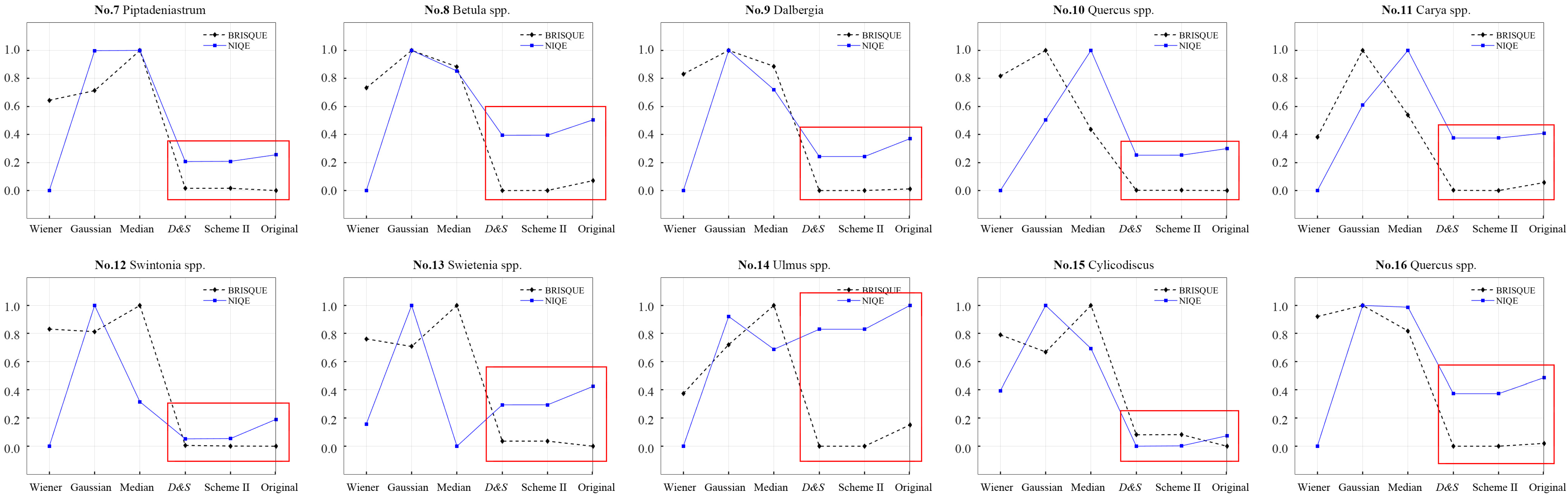
3.2.2. Evaluation of BRISQUE and NIQE

The evaluation values of BRISQUE and NIQE of the No.7 to No.16 wood images under different denoising methods are shown in

Table 7. IQA results of the No.7 to No.16 wood images under different denoising methods.

Image Number	Wiener Filtering (3 × 3)		Gaussian Filtering (3 × 3)		Median Filtering (3 × 3)		Dust & Scratches Filter		Proposed Scheme II		Original Images
	B 1	N 2	B	N	B	N	B	N	B	N	B	N
7	38.29	5.96	39.90	7.14	46.63	7.15	23.58	6.21	23.58	6.21	23.20	6.26
8	38.70	4.80	44.81	6.61	42.15	6.34	21.98	5.52	22.00	5.52	23.60	5.71
9	49.87	5.86	52.86	7.17	50.85	6.81	35.20	6.18	35.21	6.18	35.41	6.35
10	45.65	6.32	47.38	7.28	42.07	8.22	37.96	6.80	37.96	6.80	37.94	6.89
11	41.83	6.05	51.55	7.34	44.29	8.17	35.82	6.85	35.79	6.85	36.69	6.92
12	39.03	5.02	38.38	6.45	45.06	5.47	9.58	5.10	9.41	5.10	9.37	5.29
13	37.32	5.19	35.43	6.57	45.62	4.94	12.08	5.42	12.08	5.42	10.83	5.63
14	49.94	5.75	53.97	7.26	57.22	6.88	45.59	7.11	45.59	7.11	47.34	7.39
15	52.37	6.16	49.65	7.10	57.05	6.62	36.56	5.56	36.58	5.56	34.76	5.67
16	44.59	5.88	46.19	6.97	42.52	6.96	26.07	6.28	26.07	6.28	26.48	6.41

¹ B represents the evaluation values of BRISQUE; ² N represents the evaluation values of NIQE.

, and the normalization results of the corresponding values are shown in Figure 4.

It is noted that the numerical values of BRISQUE and NIQE themselves are not comparable.

From Figure 4, inside the red box, the BRISQUE values of the images denoised by Dust & Scratches filter and the proposed denoising Scheme II were close, as were the NIQE values. Nevertheless, a few of the BRISQUE values of the images denoised using the two methods were higher than the values of the corresponding original images. This might be because there a negligible amount of noise on the No.7 to No.16 wood images; denoising caused image degradation.

Outside the red box, the BRISQUE values of the images denoised using Wiener filtering, Gaussian filtering, and median filtering remained higher, while some of the NIQE values were still abnormally low, which further confirmed the inaccuracy of the evaluation of NIQE on wood image quality.

3.3. Comparison to the Originals

To compare the difference between the processed images and the corresponding original images, the structural similarity (SSIM) [28] measure, based on the spatially localized measure of correlation in pixel values [29] was introduced.

A higher SSIM value means the structure of the processed image closely matches that of the original image, whereas a lower value means less structural similarity to the original. The SSIM values of the No.1 to No.16 wood images under different denoising methods are shown in

Table 8. SSIM values of the No.1 to No.16 wood images under different denoising methods.

Image Number	Wiener Filtering	Gaussian Filtering	Median Filtering	Dust & Scratches Filter	Proposed Scheme I and II	Original Images
1	0.9757	0.9775	0.9551	0.9952	0.9926	1
2	0.9778	0.9806	0.9610	0.9961	0.9945	1
3	0.9756	0.9797	0.9555	0.9974	0.9932	1
4	0.9724	0.9772	0.9558	0.9957	0.9949	1
5	0.9813	0.9864	0.9695	0.9986	0.9977	1
6	0.9723	0.9777	0.9533	0.9949	0.9971	1
7	0.9878	0.9865	0.9828	0.9989	0.9989	1
8	0.9915	0.9899	0.9862	0.9990	0.9989	1
9	0.9936	0.9923	0.9899	0.9993	0.9993	1
10	0.9936	0.9927	0.9915	0.9995	0.9995	1
11	0.9910	0.9894	0.9857	0.9996	0.9995	1
12	0.9725	0.9715	0.9623	0.9966	0.9963	1
13	0.9856	0.9847	0.9800	0.9964	0.9964	1
14	0.9793	0.9775	0.9701	0.9966	0.9965	1
15	0.9915	0.9886	0.9858	0.9966	0.9965	1
16	0.9920	0.9910	0.9889	0.9995	0.9995	1

.

As seen in Table 8, the SSIM values of the images denoised using the Dust & Scratches filter and the proposed Scheme I and II were both closer to those of the originals. There could be changes in the relationships among the image pixels after the color substitution, leading to lower SSIM values of the proposed Scheme compared to those of the Dust & Scratches filter.

The differences in SSIM of the wood images No.1 to No.6 between the proposed Scheme and the Dust & Scratches filter were larger than the differences of the No.7 to No.16 wood images. This further confirmed that the noise was more distributed on the No.1 to No.6 wood images and verified the effectiveness of the color substitution method.

Overall, the No.1 to No.16 wood images denoised by the proposed Scheme showed more structural similarity to the originals in both subjective and objective evaluations.

4. Conclusions

The realistic noise on real-world noisy images captured by CCD cameras is complex due to the various factors in digital camera pipelines. In this paper, a novel denoising scheme for scanned wood grain images was proposed. It reduces visible noise by substituting dissimilar pixels within a certain window size in the spatial domain.

The No.1 to No.6 wood images denoised using Wiener filtering, Gaussian filtering, and median filtering exhibited ambiguity in varying degrees, and the BRISQUE values of these images were also higher. The images denoised using the Dust & Scratches filter at settings of 1 (pixels) and 35 (levels) and the proposed denoising Scheme I did not show fuzziness, but in terms of their denoising effects, the proposed Scheme I was better. The BRISQUE and NIQE values of these images were close and lower than the values of the corresponding original images, suggesting that the wood images denoised by the two methods were all improved. The results of subjective observation and objective evaluation indicated that the proposed Scheme I could reduce the randomly generated noise on the scanned wood images through color substitution, while preserving the texture details of the wood images with visible noise.

For the No.7 to No.16 wood images denoised using Wiener filtering, Gaussian filtering, and median filtering, the subjective and objective evaluations of them were consistent with those of the No.1 to No.6 wood images denoised by the three methods. There were negligible subjective visual differences between the images denoised by the Dust & Scratches filter at settings of 1 (pixels) and 35 (levels) and the proposed denoising Scheme II. The BRISQUE and NIQE values of these images were also close. The results of subjective observation and objective evaluation indicated that the denoising effect of the proposed Scheme II was consistent with that of the Dust & Scratches filter on the wood images with visually unapparent noise.

The scanned wood images were classified and sorted based on the size of luminance noise, and the classification denoising results showed that the ranges of $\alpha \ge 100$ and $\beta \le 30$ were suitable for the No.1 to No.16 wood images. Experiments demonstrated that for wood images scanned within the same batch, priority could be given to the analysis and denoising of images with evident noise.

This study focuses on the luminance noise on natural images, i.e., scanned wood grain images, and the ranges of $\alpha$ and $\beta$ in this paper are only applicable to the denoising of wood images scanned by the Microtek Phantom 9900XL scanner. It is not difficult to find that through adjusting the denoising ranges and the size of noise-searching window, the proposed Scheme can also be applied to the denoising of other types of natural images with luminance noise.

For the other types of noise that may occur on real-world wood images, the method of color substitution may not be appropriate when the relationships among natural image pixels are particularly emphasized. Moreover, the state-of-the-art denoising methods on reducing realistic noise and their computational time should be compared with the proposed Scheme in the future studies.

References

1. Slabohm, M.; Mai, C.; Militz, H. Bonding Acetylated Veneer for Engineered Wood Products—A Review. Materials 2022, 15, 3665. [Google Scholar] [CrossRef] [PubMed]
2. Sang, R.; Manley, A.; Wu, Z.; Feng, X. Digital 3D Wood Texture: UV-Curable Inkjet Printing on Board Surface. Coatings 2020, 10, 1144. [Google Scholar] [CrossRef]
3. Abdul Hamid, L.B.; Mohd Khairuddin, A.S.; Khairuddin, U.; Ruthfalydia, N.; Mokhtar, N. Texture image classification using improved image enhancement and adaptive SVM. Signal Image Video Process 2022, 16, 1587–1594. [Google Scholar] [CrossRef]
4. Rajagopal, H.; Mohd Khairuddin, A.S.; Mokhtar, N.; Ahmad, A.; Yusof, R. Application of image quality assessment module to motion-blurred wood images for wood species identification system. Wood Sci. Technol. 2019, 53, 967–981. [Google Scholar] [CrossRef]
5. Gou, H.; Swaminathan, A.; Wu, M. Intrinsic Sensor Noise Features for Forensic Analysis on Scanners and Scanned Images. IEEE Trans. Inf. Forensics Secur. 2009, 4, 476–491. [Google Scholar]
6. Suneetha, A.; Reddy, E.S. Robust Gaussian Noise Detection and Removal in Color Images using Modified Fuzzy Set Filter. J. Intell. Syst. 2020, 30, 240–257. [Google Scholar] [CrossRef]
7. Gunawan, R.; Tran, Y.; Zheng, J.; Nguyen, H.; Chai, R. Image Recovery from Synthetic Noise Artifacts in CT Scans Using Modified U-Net. Sensors 2022, 22, 7031. [Google Scholar] [CrossRef] [PubMed]
8. Mao, J.; Wu, Z.; Feng, X. Image Definition Evaluations on Denoised and Sharpened Wood Grain Images. Coatings 2021, 11, 976. [Google Scholar] [CrossRef]
9. Wen, J.; Li, Z.; Xiao, J. Noise removal in tree radar B-scan images based on Shearlet. Wood Res. 2020, 65, 1–12. [Google Scholar] [CrossRef]
10. Tan, Z.; Yang, H. Total variation regularized multi-matrices weighted Schatten p-norm minimization for image denoising. Appl. Math. Model. 2023, 124, 518–531. [Google Scholar] [CrossRef]
11. Dabov, K.; Foi, A.; Katkovnik, V.; Egiazarian, K. Color image denoising via sparse 3D collaborative filtering with grouping constraint in luminance-chrominance space. In Proceedings of the 2007 IEEE International Conference on Image Processing (ICIP), San Antonio, TX, USA, 16–19 September 2007; pp. 313–316. [Google Scholar]
12. Xu, J.; Zhang, L.; Zhang, D.; Feng, X. Multi-channel weighted nuclear norm minimization for real color image denoising. In Proceedings of the 2017 IEEE International Conference on Computer Vision (ICCV), Venice, Italy, 22–29 October 2017; pp. 1105–1113. [Google Scholar]
13. Xu, J.; Zhang, L.; Zhang, D. A trilateral weighted sparse coding scheme for real-world image denoising. In Proceedings of the European Conference on Computer Vision (ECCV), Munich, Germany, 8–14 September 2018; pp. 20–36. [Google Scholar]
14. Zoran, D.; Weiss, Y. From learning models of natural image patches to whole image restoration. In Proceedings of the 2011 IEEE International Conference on Computer Vision (ICCV), Barcelona, Spain, 6–13 November 2011; pp. 479–486. [Google Scholar]
15. Buades, A.; Coll, B.; Morel, J.M. A non-local algorithm for image denoising. In Proceedings of the 2005 IEEE Computer Society Conference on Computer Vision and Pattern Recognition (CVPR), San Diego, CA, USA, 20–25 June 2005; pp. 60–65. [Google Scholar]
16. Abdul Hamid, L.B.; Rosli, N.R.; Mohd Khairuddin, A.S.; Mokhtar, N.; Yusof, R. Denoising module for wood texture images. Wood Sci. Technol. 2018, 52, 1539–1554. [Google Scholar] [CrossRef]
17. Nam, S.; Hwang, Y.; Matsushita, Y.; Kim, S.J. A holistic approach to cross-channel image noise modeling and its application to image denoising. In Proceedings of the 2016 IEEE Conference on Computer Vision and Pattern Recognition (CVPR), Las Vegas, NV, USA, 26 June–1 July 2016; pp. 1683–1691. [Google Scholar]
18. Fraser, B.; Schewe, J. Chapter Two: Why do we sharpen? In Real World Image Sharpening with Adobe Photoshop, Camera Raw, and Lightroom; Fraser, B., Schewe, J., Eds.; Peachpit Press: Berkeley, CA, USA, 2010; pp. 11–88. [Google Scholar]
19. Li, S.; Kang, X.; Hu, J. Image Fusion with Guided Filtering. IEEE Trans. Image Process. 2013, 22, 2864–2875. [Google Scholar] [PubMed]
20. Li, J.; Zhang, X.; Li, S.; Wu, Z. Underwater color image enhancement based on two-scale image decomposition. J. Image Graph. 2021, 26, 0787–0795. [Google Scholar]
21. Mao, J.; Wu, Z.; Feng, X. A Modeling Approach on the Correction Model of the Chromatic Aberration of Scanned Wood Grain Images. Coatings 2022, 12, 79. [Google Scholar] [CrossRef]
22. Moorthy, A.K.; Bovik, A.C. A two-step framework for constructing Blind Image Quality Indices. IEEE Signal Process. Lett. 2010, 17, 513–516. [Google Scholar] [CrossRef]
23. Mittal, A.; Moorthy, A.K.; Bovik, A.C. Blind/Referenceless Image Spatial Quality Evaluator, Signals, Systems & Computers. In Proceedings of the Forty Fifth Asilomar Conference on Signals, Systems and Computers (ASILOMAR), Pacific Grove, CA, USA, 6–9 November 2011; pp. 723–727. [Google Scholar]
24. Mittal, A.; Soundararajan, R.; Bovik, A.C. Making a completely blind image quality analyzer. IEEE Signal Process. Lett. 2013, 20, 209–212. [Google Scholar] [CrossRef]
25. Moorthy, A.K.; Bovik, A.C. Blind Image Quality Assessment: From Natural Scene Statistics to Perceptual Quality. IEEE Trans. Image Process. 2011, 20, 3350–3364. [Google Scholar] [CrossRef] [PubMed]
26. Mittal, A.; Moorthy, A.K.; Bovik, A.C. No-Reference Image Quality Assessment in the Spatial Domain. IEEE Trans. Image Process. 2012, 21, 4695–4708. [Google Scholar] [CrossRef] [PubMed]
27. Gonzalez, R.C.; Woods, R.E. Digital Image Processing, 3rd ed.; Gonzalez, R.C., Woods, R.E., Eds.; Pearson Prentice Hall: Upper Saddle River, NJ, USA, 2008; pp. 112–916. [Google Scholar]
28. Wang, Z.; Bovik, A.C.; Sheikh, H.R.; Simoncelli, E.P. Image quality assessment: From error visibility to structural similarity. IEEE Trans. Image Process. 2004, 13, 600–612. [Google Scholar] [CrossRef] [PubMed]
29. Larson, E.C.; Chandler, D.M. Most apparent distortion: Full-reference image quality assessment and the role of strategy. J. Electron. Imaging 2010, 19, 011006. [Google Scholar]
Figure 1. The noise-searching window for the scanned planes from No.1 to No.16: (a) the 7 × 7 window; (b) the 5 × 5 window.
Forests 14 01803 g001
Figure 2. Algorithm flow chart.
Forests 14 01803 g002
Figure 3. The changing trends of normalized BRISQUE and NIQE values of the No.1 to No.6 wood images under different denoising methods. D&S represents Dust & Scratches filter at settings of 1 (pixels) and 35 (levels).
Forests 14 01803 g003
Figure 4. The changing trends of normalized BRISQUE and NIQE values of the No.7 to No.16 wood images under different denoising methods. D&S represents Dust & Scratches filter at settings of 1 (pixels) and 35 (levels).
Forests 14 01803 g004