Article

Assessment of Forest Ecological Function Levels Based on Multi-Source Data and Machine Learning

1
College of Mathematics and Computer Science, Zhejiang A&F University, Hangzhou 311300, China
2
Key Laboratory of State Forestry and Grassland Administration on Forestry Sensing Technology and Intelligent Equipment, Hangzhou 311300, China
3
Key Laboratory of Forestry Intelligent Monitoring and Information Technology of Zhejiang Province, Hangzhou 311300, China
4
Zhejiang Public Information Industry Co., Ltd., Hangzhou 310000, China
5
College of Economic and Management, Zhejiang A&F University, Hangzhou 311300, China
*
Author to whom correspondence should be addressed.
Forests 2023, 14(8), 1630; https://doi.org/10.3390/f14081630
Submission received: 26 June 2023 / Revised: 24 July 2023 / Accepted: 10 August 2023 / Published: 12 August 2023
(This article belongs to the Special Issue Applications of Artificial Intelligence in Forestry)

Abstract

:
Forest ecological function is one of the key indicators reflecting the quality of forest resources. The traditional weighting method to assess forest ecological function is based on a large amount of ground survey data; it is accurate but costly and time-consuming. This study utilized three machine learning algorithms to estimate forest ecological function levels based on multi-source data, including Sentinel-2 optical remote sensing images and digital elevation model (DEM) and forest resource planning and design survey data. The experimental results showed that Random Forest (RF) was the optimal model, with overall accuracy of 0.82, recall of 0.66, and F1 of 0.62, followed by CatBoost (overall accuracy = 0.82, recall = 0.62, F1 = 0.58) and LightGBM (overall accuracy = 0.76, recall = 0.61, F1 = 0.58). Except for the indicators from remote sensing images and DEM data, the five ground survey indicators of forest origin (QI_YUAN), tree age group (LING_ZU), forest category (LIN_ZHONG), dominant species (YOU_SHI_SZ), and tree age (NL) were used in the modeling and prediction. Compared to the traditional methods, the proposed algorithm has lower cost and stronger timeliness.

1. Introduction

As one of the most important components of the ecosystem, forests provide the basic natural resource foundation for the sustainable development of human beings [1]. The forest ecological function index can comprehensively reflect the structure and ecological benefits of forests. Therefore, establishing a scientific and dynamic comprehensive system to evaluate forest ecological functions plays an important role in accurately addressing ecological and economic development [2]. As research progresses, a single analysis of a particular forest characteristic no longer meets the current requirements. Therefore, it is important to assess forests’ ecological functions by integrating the synergistic effects of multiple factors [3,4]. Many scholars have attempted to present concepts or tools for forest ecological function analysis [5,6,7], greatly helping to measure and quantify species’ actions.
Currently, some progress in the quantitative estimation of forest ecological functions has been made in China. In terms of research methods, Li Ma et al. established the Beijing Forest Ecosystem Health Evaluation Index System (EIS-BFEH) to evaluate the health function of forest ecosystems and used the hierarchical analysis process (AHP) to obtain a comprehensive index (CI) representing the health status of forest ecosystems [8]. Fang Xiaomin et al. used a comprehensive index method and a statistical grouping method to evaluate forest functions and calculated the forest ecological function index to compare forest ecological functions for different age groups, species structure, and origin [9]. Du Qun et al. proposed that the three factors of forest quantity, quality, and spatial distribution should be used for forest ecological function evaluation [10]. Although there has been some progress in research on computational methods and evaluation factors, the current studies are mainly focused on simple statistical methods, and there is a lack of attempts of using machine learning methods; this procedure cannot meet the requirements of accurately evaluating and monitoring forest ecological functions based on multi-data [11].
Among machine learning algorithms, ensemble learning algorithms can combine multiple classifiers together to improve the accuracy and generalization ability of classifiers. Overall, based on the presence or absence of dependencies between base classifiers, ensemble learning algorithms are divided into two types: boosting and bagging. Boosting algorithms have a strong dependency between base classifiers, and a series of base classifiers needs to be generated serially, represented by AdaBoost and GBDT. In fact, GBDT is more suitable for multi-category classification, and LightGBM and CatBoost are two important improved algorithms based on GBDT. In contrast, bagging algorithms do not have a strong dependency between base classifiers, and a series of base classifiers can be generated in parallel, represented by Random Forest. Regarding the research data, Wang Daling et al. evaluated the forest ecological function of arboreal forests based on the data of subcompartments from the 2018 forest resources planning and design survey of the Sanchazi Forestry Bureau [12]. Jun Yang et al. conducted a qualitative analysis of the health and ecological status of Chinese forests in 2009 based on the data of the seventh national forest resource inventory [13]. Liu Lixia et al. evaluated the ecological functions of forests based on the data of the forest resources planning and design survey [14]. Zhang Xianwu et al. used the results of the three continuous forest inventories from 2004, 2009, and 2014 to analyze the current situation, changes, and reasons of changes in the comprehensive index of forest ecological functions in Shanghai using nine indicators including forest stock, forest naturalness, and proportion of forest land area to national land area [15]. Even though forest resource inventory data has high accuracy, there are still issues of high cost and difficulty in data acquisition. Forest managers, decision makers, and politicians need to be able to make data-driven rapid decisions based on short-term and long-term monitoring information, complex modeling, and analysis approaches [11]. Thus, researchers are increasingly considering incorporating lower-cost data such as remote-sensing images and lower-cost strategies into our study.
It is necessary to attempt to integrate multi-source data to evaluate the forest ecological function. In recent years, the application of multi-source data fusion in the forestry field has become increasingly common, indicating that multi-source data have broad application prospects. For instance, Wang et al. used multi-source remote sensing data (Gaofen 1, Sentinel-2, Landsat 9, and Gaofen 3) to classify mangrove species in urban areas of Leizhou City, Guangdong Province [16]; Abd Rahman Kassim et al. used hyperspectral images and airborne LiDAR data to evaluate the ecological status of the FRIM campus forest ecosystem [17]. Some of the studies on multi-source data fusion in the field of forestry have achieved good results, but there is still more room to explore its application in forest ecological function level assessment.
This paper aimed to combine multi-source data with machine learning algorithms to assess the forest ecological function levels based on the unit of forest subcompartment. Spectral features and topographic features of the study area were collected from remotely sensed images and DEM. Some ground data with low acquisition cost, such as forest origin, tree age group, forest category, dominant species, and tree age, were provided by the forest resource planning and design survey. Based on the multi-source data scheme, three classic machine learning algorithms, i.e., Random Forest, LightGBM, and CatBoost, were involved in the study.

2. Materials and Methods

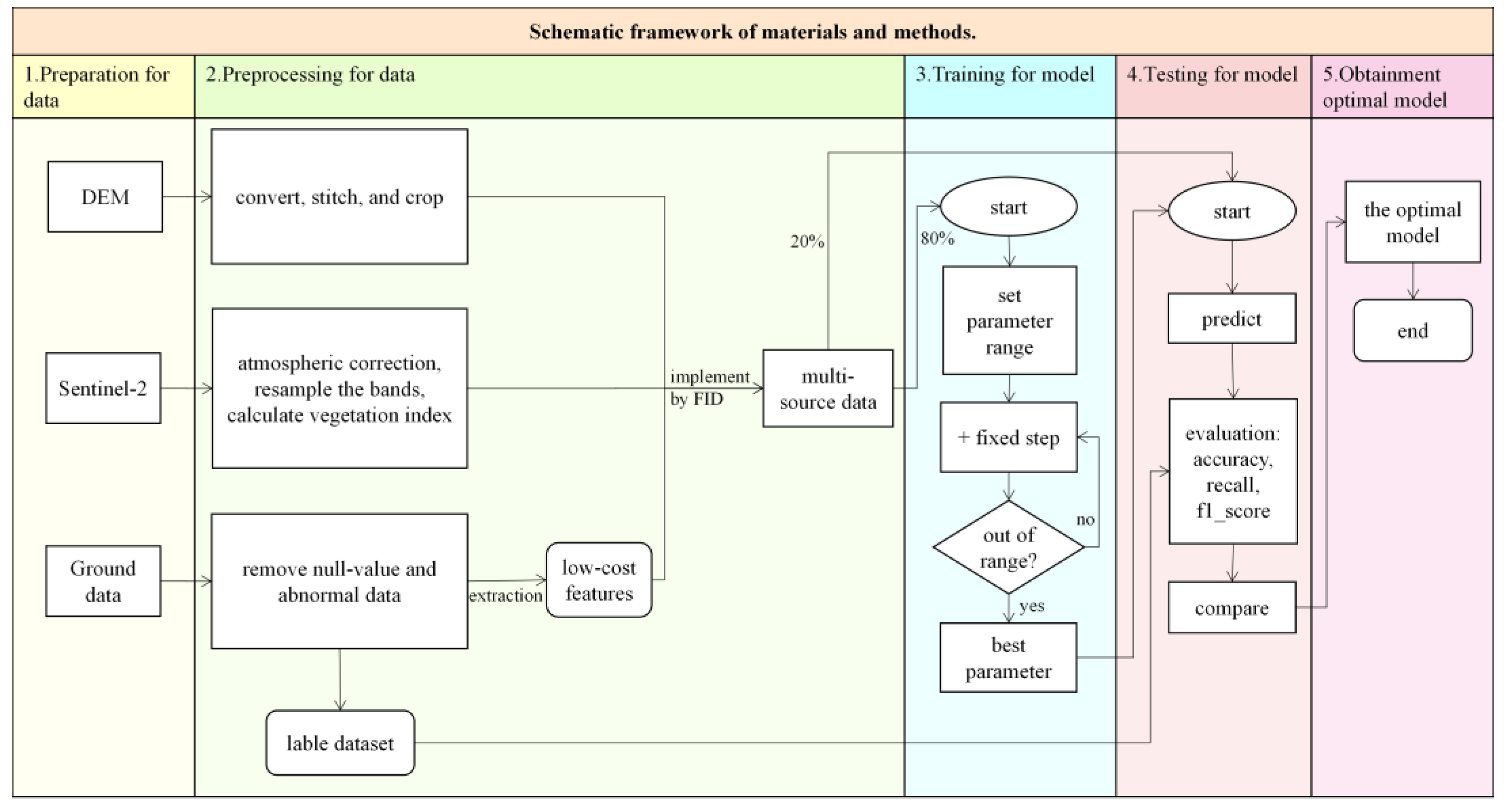
2.1. Schematic Framework of Materials and Methods

The schematic framework of the Materials and Methods of this study is shown in Figure 1, including multi-source data, preprocessing methods, models to predict forest ecological function levels.

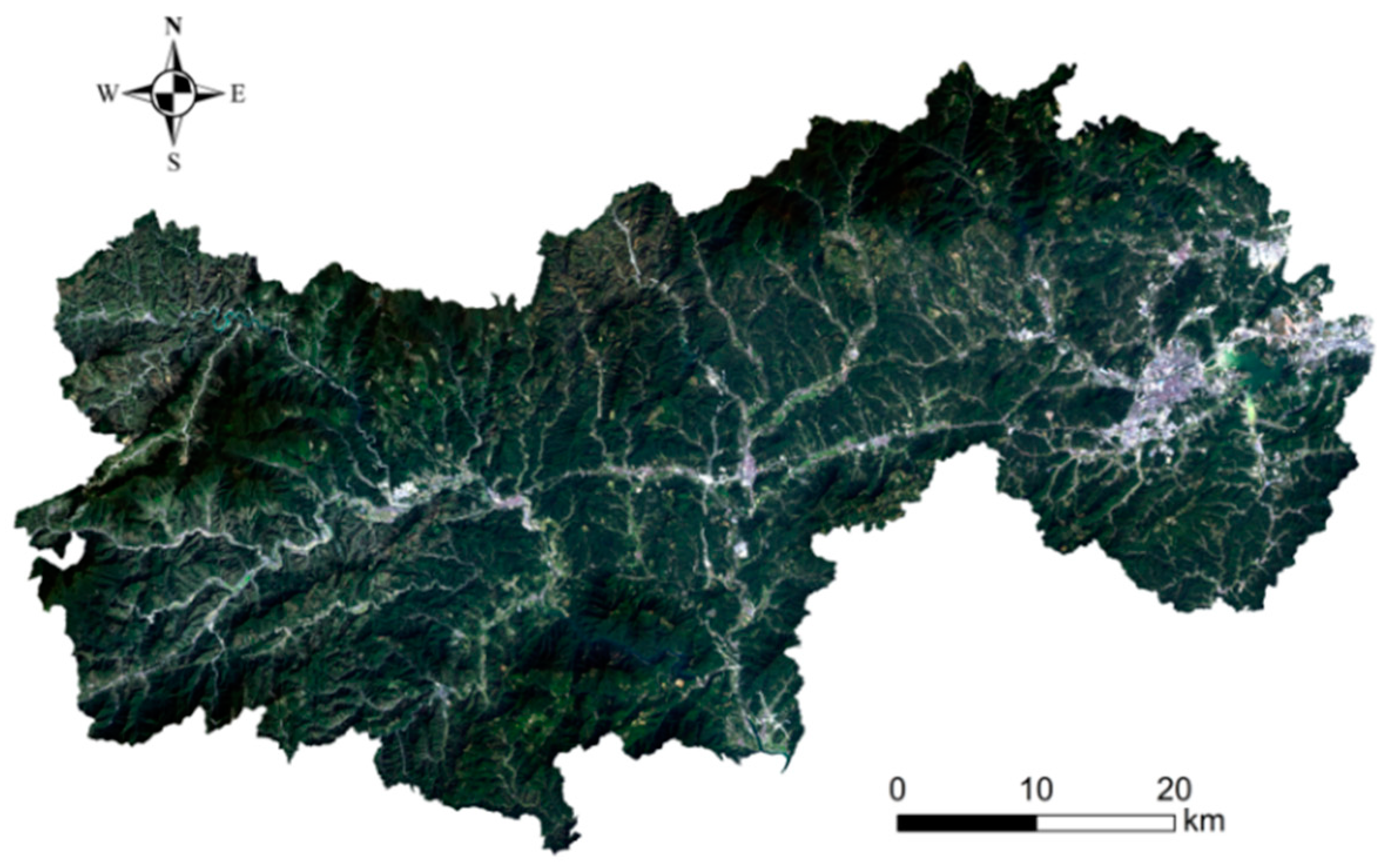
2.2. Overview of the Study Area

Lin’an District (118°51′~119°52′ E, 29°56′~30°23′ N) is located in the northwest of Zhejiang Province, with a total area of 3126.8 square kilometers, shown in Figure 2. It is in the central subtropical monsoon climate zone, rich in plant resources. As a typical southern forest city, the forestry land area of Lin’an is up to 263,868.79 hm2, with 1603.88 hm3 of forest standing stock and 81.99% of forest canopy density.

2.3. Processing of Label Dataset

According to the Technical Operation Rules for forest resources planning and design survey of Zhejiang Province of 2014 [18] and the Technical Regulations for the Continuous Inventory of Forest Resources of 2020 (GB/T 38590-2020) [19], there are eight investigation factors (Table 1), i.e., forest biomass, forest naturalness, forest community structure, tree species structure, vegetation coverage, forest canopy density, mean tree height, and thickness of dead leaves, involved into the traditional algorithm to evaluate a forest ecological function levels. Their weights were determined according to their importance to the evaluation of forest ecological functions (Table 1).
To facilitate the data standardization, the values of the above eight evaluation factors were uniformly classified into three classes, i.e., Ⅰ, Ⅱ, and Ⅲ. According to the data type and the distribution of the values, the above eight evaluation factors were divided into three categories. The first category, including vegetation coverage, canopy density, mean tree height, forest community structure, and thickness of dead leaves, was directly classified into types Ⅰ, Ⅱ, and Ⅲ (as shown in Table 1). The second category. consisting of forest naturalness and tree species structure, was classified first by the division standards of Table 2 for naturalness and Table 3 for tree species structure, and then into types of Ⅰ, Ⅱ, and Ⅲ. The third category merely included forest biomass, which was firstly calculated according to the amount of forest volume for various dominant species by equations (shown in Table 4) and then classified into types Ⅰ, Ⅱ, and Ⅲ.

2.4. Data Sources and Pre-Processing

2.4.1. Data Sources

The data sources mainly included remote sensing images and Digital Elevation Model and ground survey data. The remote sensing images from the satellite Sentinel-2 (with 13 Bands, a spatial resolution of 10 m, 20 m, and 60 m) and DEM (with a spatial resolution of 30 m) with a format of ASTER GDEM, were all downloaded from the International Science and Technology Data Mirror of the Computer Network Information Centre of the Chinese Academy of Sciences (www.gscloud.cn) on 27 September 2021. The ground data were obtained from the forest resources planning and design survey provided by the Lin’an District Forestry Bureau in 2019.

2.4.2. Data Pre-Processing

(1)
Forest Resources Planning and Design Survey Data
The original data of forest resource planning and design survey consist of 119,792 sub-compartments. To eliminate erroneous data, two steps were taken. Firstly, the data with non-forest, zero volume, and null value of forest ecological function level were removed. Secondly, according to the Pauta criterion [21], the abnormal data exceeding the mean (u) ± three times the standard deviation (3σ) were also removed. Consequently, 47,596 valid samples were retained (Table 5), consisting of 26 dominant tree species, that is, broad-leaved mixed forest, horsetail pine, fir, coniferous mixed forest, coniferous mixed forest, oak, other hard broad-leaved forest, maple, camphor, yellow pine, etc.
(2)
Extraction and processing of characteristic factors based on images from remote sensing and DEM
For the Sentinel-2 remote sensing images, Sen2Cor® (v2.8, European Space Agency, Paris, France) was used for atmospheric correction, and SNAP® (v6.0, European Space Agency, Paris, France) was exploited to resample the bands (band1, band5, band6, band7, band8A, band9, band10, band11, and band12) to fuse the lower-resolution images of 20 m and 60 m with higher-resolution images of 10 m by the nearest neighbor method. After that, by the operations of image mosaic and clipping in ArcGIS® (v10.8, Environmental Systems Research Institute, Inc., Redlands, CA, USA), a valid and complete remote sensing image of the Lin’an District (Figure 3) was produced.
The characteristic factors extracted from the Sentinel-2 optical remote sensing images consisted of two main types: original factors and derived factors. The former consisted of 13 bands [22,23,24]. There were three bands, namely, Band1 for the coastal band, Band9 for the water vapor band, and Band10 for the cirrus band, which were not relevant to the experiment and were removed. Therefore, the remaining ten original bands (as shown in Table 6) and eleven vegetation indices-derived factors (as shown in Table 7), that is, a total of 21 spectral feature factors, were used as independent variables.
In this study, the remote sensing images and DEM were preprocessed by converting, stitching, and cropping in ArcGIS. The three topographic factors—elevation, slope, and aspect—were obtained from DEM images (Figure 4), with a spatial resolution of 30 m.

2.5. Extraction of Feature Factors from Ground Survey Data

Even if the forest Resources Planning and Design Survey data have authenticity and reliability, many factors, such as forest biomass, vegetation coverage, forest canopy density, and mean tree height, with very high investigation costs, are not suitable for evaluating forest ecological function levels. Therefore, the eight factors (shown in Table 1) which were traditionally used to compute forest ecological function levels were removed, and unrelated factors such as county code and county name were also removed. After that, 36 variables remained. To further reduce the dimensionality of the features and improve the efficiency of the model, the feature importance was ranked (as shown in Figure 5). Furthermore, five feature factors, that is, QI_YUAN, LING_ZU, NL, YOU_SHI_SZ, and LIN_ZHON, were selected as independent variables of the model from top to bottom.

2.6. Multi-Source Data Integration

A total of 29 evaluation factors (as shown in Table 7) were involved in the study, including 10 spectral bands, 11 vegetation indices, 5 ground survey factors, and 3 topographic factors. The integration of the multi-source data was implemented according to the FID.
Finally, the dataset was randomly divided into a training set with 80% of the samples for modeling and a test set with 20% of the samples for testing.

2.7. Methods

2.7.1. Grid SearchCV

To prevent overfitting and underfitting, a hyper-parameter optimization method—grid search (Grid SearchCV [25])—was used to select the optimal hyper-parameter values for the three models. Grid SearchCV allows performing hyperparameter tuning in order to determine the optimal values for a given model. Specifically, based on a specified parameter range and a validation dataset, the parameters are gradually adjusted based on a pre-set step size, and finally the optimal parameter value was selected with the highest accuracy.

2.7.2. Random Forest (RF)

Random forest [26,27] is a collection of multiple decision tree algorithms with random sampling, which is a combination of Breiman’s “bagging” idea and a random selection of features. The procedure consists in making a precise prediction by taking the average or mode of the output of multiple decision trees (shown in Figure 6). Typically, the greater the decision trees’ number, the more precise the output and the greater the overhead. In our study, to balance accuracy and overhead, the default number of decision trees was set to 100, and the parameter range of the grid search was set to 100–500 with a step size of 5. The final experimental results showed that when the number of subtrees reached 200, the increase in the number of subtrees had a minimal effect on the model enhancement. Therefore, the optimal parameter value was finally set to 200. Also, the maximum number of features was set to 195, which was the square root of the number of training samples (47,596 * 0.8).

2.7.3. Light Gradient Boosting Machine (LightGBM)

The Light Gradient Boosting Machine, XGBoost, and Catboost are lifting algorithms [28]. For the LightGBM, during the training process, the decision tree algorithm of Histogram was adopted, which greatly reduced the calculation amount of the model. Meanwhile, the leaf-wise growth strategy (shown in Figure 7) was introduced into the growth process of the subtree, which reduced the splitting of invalid nodes.
There are three hyperparameters in LightGBM that need to be determined through the grid search method, namely, n_estimators, max_depth, and learning_rate. Here, n_estimators is the maximum number of base learners, max_depth is the maximum depth of the tree, and learning_rate indicates the magnitude of each parameter update. Correspondingly, the parameter ranges were set to [100, 300], [2, 10], and [0.05, 0.2], with step sizes of 5, 1, and 0.01, respectively. Finally, the optimal values of the three parameters were 200 for n_estimators, 3 for max_depth, and 0.1 for learning_rate, respectively.

2.7.4. CatBoost

CatBoost [29,30] is a GBDT algorithm based on a symmetric binary tree, which can automatically process category-based features and effectively solve gradient bias and prediction shift problems and has excellent accuracy and generalization capabilities. In addition, CatBoost combines multiple categorical features by adding a priori distributed modified Greedy TS approach to reduce the effect of noise and low-frequency categorical data on the data distribution (as calculated in Equation (1)).
X σ p , k = p 1 j = 1 [ X σ j , k = X σ p , k ] Y σ j + a × p p 1 j = 1 [ X σ j , k = X σ p , k ] + a
where a is a weighting factor greater than 0; p is the priori.
The default value of n_estimators in CatBoost package we used was 500, which was already large enough. For the other two parameters, tree depth and learning rate, their ranges were set to [5, 12] and [0.05, 0.2], with step sizes of 1 and 0.01, respectively. Consequently, the optimal tree depth was 11, and the learning rate was 0.05.

2.7.5. Performance Metrics

The performance metrics of the model are generally calculated based on a confusion matrix [31], as shown in Table 8. Here, a i j denotes the number of samples, the measured value is denoted by i , and the predicted value is denoted by j , N is the total number of samples, k is the number of target categories, and a i + = j a i j , a + j = i a i j .
Furthermore, the performance of the predicted results was evaluated by accuracy (Formulas (3)), recall (Formulas (5)), and F1_score (Formulas (8)).
a c c u r a c y i = a i i N
a c c u r a c y = i = 1 k a c c u r a c y i
r e c a l l i = a i i a + i
r e c a l l = i = 1 k r e c a l l i
p r e c i s i o n i = a i i a i +
F 1 _ s c o r e i = 2 p r e c i s i o n i r e c a l l i p r e c i s i o n i + r e c a l l i
F 1 _ s c o r e = i = 1 k F 1 _ s c o r e i

3. Results

3.1. Labeling of the Data

The quantification scores for Type I, II, and III in Table 1 were assigned to 1, 2, and 3, respectively [32], and the composite score of forest ecological functions were calculated according to Formula (9) [19]
Y = i = 1 8 W i X i
where Y is the composite score of the forest, X i is the standardized score of the i-th evaluation factor, and W i is the weight of the i-th evaluation factor.
Hence, the ecological function index was calculated according to the composite score and is represented by Equation (10)
K = 1 Y
where K is the the ecological function index with a value less than or equal to 1. The larger the value of K , the better the forest’s ecological function.
Further, according to the values of K , the ecological function levels were divided into three groups, i.e., Good, Medium, and Poor (as shown in Table 9).
Consequently, the classification results based on Equation (10) acted as the labeled data and were plotted in Figure 8. As shown, 10,844 forest subcompartments were graded as “good”, 36,365 forest subcompartments were graded as “medium”, and 386 forest subcompartments were graded as “poor”. In terms of area, the ecological function levels of “good”, “medium”, and “poor” were 59,094.3 hectares, 92,011.9 hectares, and 487.6 hectares, respectively, accounting for 38.98%, 60.70%, and 0.32% of the total area of forest land, respectively. The average forest ecological function index of forested land in Lin’an was 0.63, which was only 0.04 lower than the good ecological function index of 0.67, and the overall ecological function was at a medium, tending to good, level.
There was an upward tendency for forest ecological function levels from east to west, which was consistent with the zoning of construction land in Lin’an District, with more urban construction land to the east and more ecological forest areas to the west. The extent to which the experimental results were consistent with the actual situation from the cross-reference map of the focus areas (Figure 9) was determined. For example, the two national nature reserves in Figure 9a,b corresponded to areas where the ecological function of the forest was rated as “good” on a large scale and, partly, as “medium”, with no areas rated as “poor”. Closer to urban areas, there was a greater chance of a “poor” forest ecological function level (as shown in Figure 9c). To some extent, this reflected the impact of human activities on the levels of forest ecological function. The regions with lower human activity often had higher levels of forest ecological function, while the regions with higher human activity had lower levels of forest ecological function.

3.2. Design of the Data Scheme

Four data combination schemes (as shown in Table 10)—A, B, C, and D—were designed according to the three data sources.

3.3. Testing Results

The results of the optimal hyperparameters for three models were obtained by grid search (Section 2.7 for details), as shown in Table 11. Furthermore, the four different data combination schemes (shown in Table 10) were modeled and analyzed using the random forest, LightGBM, and CatBoost algorithms, and the experimental results are shown in Table 12.
Comparing the performance metrics of the four data schemes in the three models in Table 12, the data scheme A (single-data combination scheme) had the worst performance, with an overall accuracy rate of only 0.46~0.47 and a classification accuracy of 0.32~0.35 for the “poor” category samples. However, the data scheme D (multi-source-data combination scheme) performed the best, with an overall accuracy rate of 0.76~0.82. The accuracy of the “good”, “medium”, and “poor” categories reached 0.73~0.76, 0.89~0.90, and 0.64~0.80, respectively, and the F1 score was 0.58~0.62. When comparing the data scheme B (after adding the DEM data to scheme A) with A, it was found that the DEM had an insignificant contribution to the model, with an overall accuracy improvement of only 0.01~0.02, and the accuracy of the “good”, “medium”, and “poor” categories, respectively, improved by 0.01~0.16, 0~0.01, and 0.01~0.07. However, when comparing the data scheme C (after adding the ground survey data to scheme A) with A, it was found that the addition of the forest resource planning and design survey data made a significant positive contribution to the model, with an overall accuracy improvement of 0.26~0.36, significantly improving the performance metrics of “good”, “medium”, and “poor” categories, respectively.
Ultimately, the RF-D executed the optimal program with overall accuracy of 0.82, recall of 0.66, and F1 score of 0.62, and the classification accuracy was significantly improved, especially for the small sample category of “poor”.

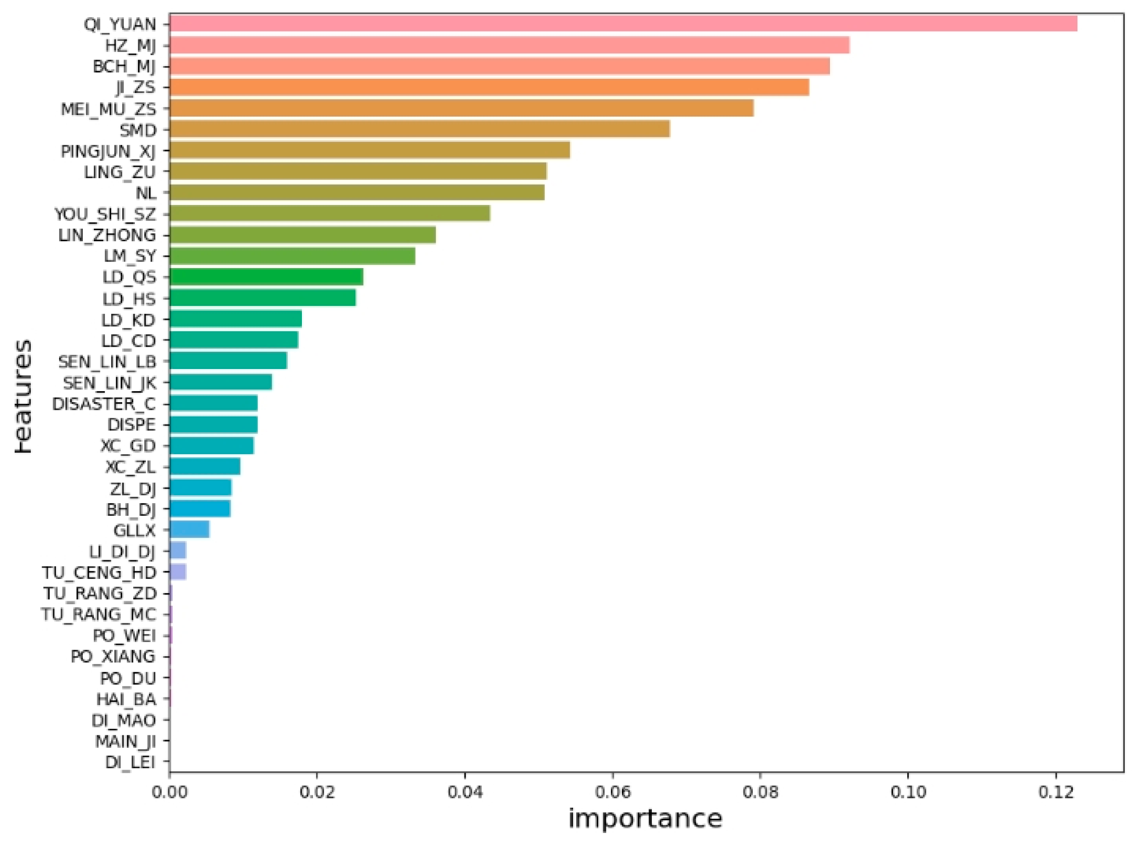
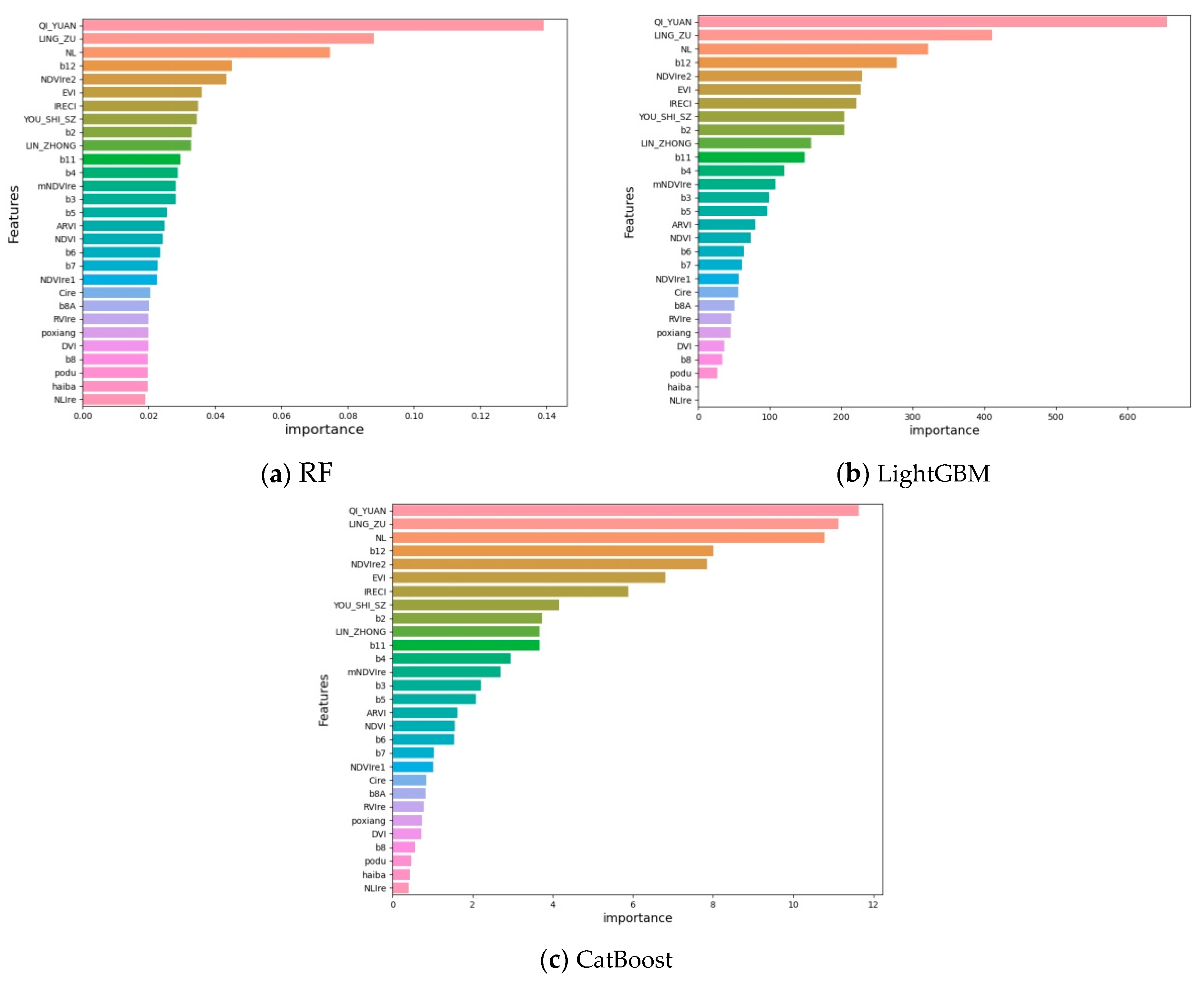
3.4. Ranking of Features’ Importance

Based on the optimal data scheme D, the performance metrics (as shown in Table 12) were calculated by the three machine learning algorithms of RF, LightGBM, and CatBoost, and the ranking of the feature importance was obtained and shown in Figure 10.
As shown in Figure 10, there were five factors from the ground survey data that led to a higher ranking of feature importance and played an important role in the model. Nevertheless, there were three factors from the DEM data with a lower ranking of feature importance that played an unimportant role in the model, which is consistent with the results in Table 11. In the optical remote sensing data, the factors of b12, NDVIre2, EVI, IRECI, b2, b11, and b4 ranked relatively high in the model.

4. Discussion

4.1. Performance Metrics

Even if many studies have been aimed to the forest ecological function rating methodology, some deficiencies still exist, as reported below.
(1)
The evaluation indicators are heavily influenced by foresters’ experience
In the evaluation of forest ecological functions, due to many qualitative indicators such as forest naturalness, tree species structure, and thickness of dead leaves, the original way of obtaining data is heavily influenced by foresters’ experience, which makes it difficult to establish an objective indicator system and may lead to inconsistent forest ecological function levels evaluated by different foresters for the same forest stand [33,34].
(2)
High cost of data acquisition for evaluation indicators
The data of the eight evaluation factors (forest naturalness, forest community structure, tree species structure, vegetation coverage, forest canopy density, mean tree height, and thickness of dead leaves) used to calculate the forest ecological function levels are obtained from ground surveys, which leads to high acquisition costs and time consumption [35].
The proposed evaluation method combined the advantages of multiple sources of data and machine learning algorithms to effectively reduce the human influence on the evaluation system and save data acquisition expenses and time. Specifically, the addition of remote sensing data effectively reduced the influence of human subjective experiences and increased the frequency of data acquisition. The costs of acquiring remote sensing data are also much lower than that of ground surveys [36], especially in areas that are difficult to access by humans, such as deep forests and cliffs.

4.2. Complementarity of Multi-Source Data

As machine learning algorithms are data-driven, variations in the data could greatly affect the accuracy of a classification [37]. When providing insufficient data, such as for data scheme A (merely optical remote sensing data from Sentinel-2), poor results were obtained (overall accuracy of 0.46~0.47 for scheme A in Table 11). Due to influences by environmental conditions such as different angles and intensities of sunlight, topography, water content, and other factors, it is possible that the same object may have different spectrums, and different objects may have the same spectrum [38,39]. For instance, the spectral information for the same vegetation on sunny and shady slopes could be different, and the height of lower vegetation is easily obscured by shadows. This tends to increase the errors during training. Complementarity of multiple sources of data is generally used to address this problem.
Compared to the data scheme A, the data scheme D (addition of DEM data and some ground survey data) significantly increased the overall accuracy by 0.29~0.36, with the accuracy rates for the “good”, “medium”, and “poor” categories increasing by 0.12~0.19, 0.09~0.1, and 0.32~0.48, respectively. The addition of DEM data complements vertical structure parameters which are lacking in optical remote sensing data [40], allowing areas of deciduous trees to be distinguished from areas of vegetation with similar spectral characteristics (e.g., high-density grassland) [41], which in turn has an impact on the accuracy of the results. The addition of ground survey data further complements the growth status information for the vegetation—such as the age of trees that can lead to changes in their growth rate—thereby improving the accuracy of the model.

4.3. The Feasibility of Machine Learning

Different from the traditional statistical methods used by Huafu Liu et al. [42], Hailong Yin et al. [43], and Kassim et al. [17], this paper exploited a machine learning algorithm to develop a comprehensive model to evaluate forest ecological function levels, which has a higher flexibility and faster processing speed for high-dimensional data with more complex relationships among feature factors. Most indicators are non-linearly related to forest ecological function levels, including ground survey factors and spectral characteristics. For instance, with the increasing NL, the forest ecological function levels increase first and then decrease. Machine learning algorithms are non-linear approximations to an objective function, different from than the traditional comprehensive evaluation methods bound to a linear function, such as the scoring method, principal component analysis, etc. Therefore, their powerful fitting ability could make the predicted results closer to the reality and improve the evaluation accuracy of the model.
The Random Forest showed the best performance among the above three models, with an overall accuracy of 0.82 and an F1 score of 0.62. As a non-linear, parametric classifier, Random Forest is robust with non-equilibrium data and can randomly generate multiple decision trees to form a forest, effectively avoiding overfitting [44,45]. It allows the fusion of high-dimensional data from multiple sources [46] and has a high tolerance for missing values and outliers, so that it can effectively reduce the interference of noise in the data. In addition, it can automatically determine the importance of variables, which in turn improves its accuracy and usability.

4.4. Limitations of this Study

This study, based on the multi-source data of Sentinel-2 remote sensing images and DEM and partial data from the forest resource planning and design survey, as well as the three machine learning algorithms RF, LightGBM, and CatBoost, evaluated the forest ecological function levels. Overall, our results may promote research on the evaluation of forest ecological function levels. However, the 10 m resolution of the Sentinel-2 images may limit a further improvement of the performance metrics. If higher-resolution images can be acquired in the future, such as remote sensing images from Gaofen series satellites or UAV images, it will be possible to further increase the performance of our model and even further reduce the participation of ground survey indicators. On the other hand, from the perspective of research methods, deep learning algorithms such as YOLO are also worth a try in the future.

5. Conclusions

Optical remote sensing data, DEM data, and forest resource planning and design survey data were used in this study to evaluate the forest ecological function levels of Lin’an District using three machine learning algorithms, i.e., RF, LightGBM, and CatBoost.
In the three models, Random Forest was the best-performing model, with an overall accuracy rate of 0.82 (the accuracy rates for the “good”, “medium”, and “poor” categories being 0.76, 0.89, and 0.83, respectively) and with an F1 score of 0.62.
The multi-source data significantly improved the performance metrics. Furthermore, the acquisition of ground survey data such as QI_YUAN, LING_ZU, LIN_ZHONG, YOU_SHI_SZ, and NL, was achieved at lower costs than those required for the traditional eight indicators of forest biomass, forest naturalness, forest community structure, tree species structure, vegetation coverage, forest canopy density, mean tree-height, and thickness of dead leaves.
If more data sources are used, such as higher-resolution remote sensing images, LiDAR remote sensing images, etc., the estimation performance might further improve in the future.

Author Contributions

Conceptualization, D.W.; Formal analysis, S.L.; data curation, L.Y.; Funding acquisition, D.W. and X.Z.; Methodology, X.Z.; Resources, L.Y.; Writing—original draft, N.F.; writing—review and editing, L.Y. All authors have read and agreed to the published version of the manuscript.

Funding

This research was financially supported by the Zhejiang Forestry Science and Technology Project (2023SY08), the National Natural Science Foundation of China (Grant No. 42001354), and the Natural Science Foundation of Zhejiang Province (Grant No. LQ19D010011).

Data Availability Statement

The remote sensing data can be found here: [https://scihub.copernicus.eu/ (accessed on 27 September 2021)]. The DEM data can be found here: [www.gscloud.cn (accessed on 13 December 2021)]. The ground survey data are not publicly available (for policy reasons, these data are kept confidential).

Conflicts of Interest

The authors declare no conflict of interest.

References

  1. Liu, Y.; Wang, S.; Chen, Z.; Tu, S. Research on the Response of Ecosystem Service Function to Landscape Pattern Changes Caused by Land Use Transition: A Case Study of the Guangxi Zhuang Autonomous Region, China. Land 2022, 11, 752. [Google Scholar] [CrossRef]
  2. Tang, Y.; Shao, Q.; Liu, J.; Zhang, H.; Yang, F.; Cao, W.; Wu, D.; Gong, G. Did Ecological Restoration Hit Its Mark? Monitoring and Assessing Ecological Changes in the Grain for Green Program Region Using Multi-source Satellite Images. Remote Sens. 2019, 11, 358. [Google Scholar] [CrossRef] [Green Version]
  3. Holling, C.S. Simplifying the complex: The paradigms of ecological function and structure. Eur. J. Oper. Res. 1987, 30, 139–146. [Google Scholar] [CrossRef]
  4. Aerts, R.; Honnay, O. Forest restoration, biodiversity and ecosystem functioning. BMC Ecol. 2011, 11, 29. [Google Scholar] [CrossRef] [Green Version]
  5. Brodie, J.F.; Redford, K.H.; Doak, D.F. Ecological Function Analysis: Incorporating Species Roles into Conservation. Trends Ecol. Evol. 2018, 33, 840–850. [Google Scholar] [CrossRef]
  6. Shen, W.; Li, M.; Huang, C.; Wei, A. Quantifying Live Aboveground Biomass and Forest Disturbance of Mountainous Natural and Plantation Forests in Northern Guangdong, China, Based on Multi-Temporal Landsat, PALSAR and Field Plot Data. Remote Sens. 2016, 8, 595. [Google Scholar] [CrossRef] [Green Version]
  7. Rizky, P.M.; Safe’i, R.; Kaskoyo, H.; Febryano, I.G. Forestry Value for Health Status: An Ecological Review. IOP Conf. Ser. Earth Environ. Sci. 2022, 995, 012002. [Google Scholar] [CrossRef]
  8. Ma, L.; Han, H.R. Evaluation of the forest ecosystem health in Beijing area. For. Stud. China 2007, 2, 157–163. [Google Scholar] [CrossRef]
  9. Fang, X.M. Evaluation of ecological functions of forests in the Aojiang River Basin. For. Surv. Des. 2022, 1, 36–39+61. [Google Scholar]
  10. Du, Q.; Ji, B.Y.; Xu, J. Research on forest ecological function evaluation based on forest quantity, quality and spatial distribution. Zhejiang For. Sci. Technol. 2013, 33, 46–50. [Google Scholar]
  11. Lausch, A.; Borg, E.; Bumberger, J.; Dietrich, P.; Heurich, M.; Huth, A.; Jung, A.; Klenke, R.; Knapp, S.; Mollenhauer, H.; et al. Understanding Forest Health with Remote Sensing, Part III: Requirements for a Scalable Multi-Source Forest Health Monitoring Network Based on Data Science Approaches. Remote Sens. 2018, 10, 1120. [Google Scholar] [CrossRef] [Green Version]
  12. Wang, D.L.; Zhang, X.; Yang, Q.; Zhang, X.Y.; Gong, J.Q.; Dong, H. Evaluation of forest ecological functions in Sanjiuzi Forestry Bureau. Jilin For. Sci. Technol. 2022, 51, 34–37. [Google Scholar]
  13. Yang, J.; Dai, G.; Wang, S. China’s National Monitoring Program on Ecological Functions of Forests: An Analysis of the Protocol and Initial Results. Forests 2015, 6, 809–826. [Google Scholar] [CrossRef]
  14. Liu, L.X.; Zhu, S.W. Evaluation of forest ecological functions in Beijing Jingxi Forestry Management Office. Green Technol. 2022, 24, 152–155. [Google Scholar]
  15. Zhang, X.W.; Zheng, C.M.; Tang, X.J.; Zhang, W.D. Comprehensive index assessment of forest ecological functions in Shanghai. Subtrop. Soil Water Conserv. 2015, 27, 34–37. [Google Scholar]
  16. Wang, X.Z.; Tan, L.L.; Fan, J.C. Performance Evaluation of Mangrove Species Classification Based on Multi-Source Remote Sensing Data Using Extremely Randomized Trees in Fucheng Town, Leizhou City, Guangdong Province. Remote Sens. 2023, 15, 1386. [Google Scholar] [CrossRef]
  17. Abd Rahman Kassim, M.A.M.; Faidi, M.A.; Omar, H. A tool for assessing ecological status of forest ecosystem. IOP Conf. Ser. Earth Environ. Sci. 2016, 37, 012026. [Google Scholar]
  18. Relevant Attachments to the Technical Regulations for Category 2 Investigation in Zhejiang Province in 2014. Available online: https://wenku.baidu.com/view/441978e3b80d6c85ec3a87c24028915f804d848a.html (accessed on 28 September 2021).
  19. GB/T 38590-2020; Technical Regulations for Continuous Inventory of Forest Resources. China National Standard Publishing House: Beijing, China, 2020; pp. 1–48.
  20. Fang, J.Y.; Wang, G.G.; Liu, G.H.; Xu, S.L. Forest biomass of China: An estimate based on the biomass-volume relationship. Ecol. Appl. 1998, 8, 1084–1091. [Google Scholar]
  21. Liu, Y.; Fan, Z.P.; You, T.H.; Zhang, W.Y. Large group decision-making (LGDM) with the participators from multiple subgroups of stakeholders: A method considering both the collective evaluation and the fairness of the alternative. Comput. Ind. Eng. 2018, 122, 262–272. [Google Scholar] [CrossRef]
  22. Keshta, A.E.; Riter, J.C.A.; Shaltout, K.H.; Baldwin, A.H.; Kearney, M.; Sharaf El-Din, A.; Eid, E.M. Loss of Coastal Wetlands in Lake Burullus, Egypt: A GIS and Remote-Sensing Study. Sustainability 2022, 14, 4980. [Google Scholar] [CrossRef]
  23. Ebodé, V.B. Land Surface Temperature Variation in Response to Land Use Modes Changes: The Case of Mefou River Sub-Basin (Southern Cameroon). Sustainability 2023, 15, 864. [Google Scholar] [CrossRef]
  24. Fernandez-Beltran, R.; Baidar, T.; Kang, J.; Pla, F. Rice-Yield Prediction with Multi-Temporal Sentinel-2 Data and 3D CNN: A Case Study in Nepal. Remote Sens. 2021, 13, 1391. [Google Scholar] [CrossRef]
  25. Sumathi, B. Grid search tuning of hyperparameters in random forest classifier for customer feedback sentiment prediction. Int. J. Adv. Comput. Sci. Appl. 2020, 11, 173–178. [Google Scholar]
  26. Yoshida, Y.; Yuda, E. Workout Detection by Wearable Device Data Using Machine Learning. Appl. Sci. 2023, 13, 4280. [Google Scholar] [CrossRef]
  27. Xiao, S.; Laurie, A.C. Classification of Australian Native Forest Species Using Hyperspectral Remote Sensing and Machine-Learning Classification Algorithms. IEEE J. Sel. Top. Appl. Earth Obs. Remote Sens. 2014, 7, 2481–2489. [Google Scholar]
  28. Han, P.; Zhai, Y.; Liu, W.; Lin, H.; An, Q.; Zhang, Q.; Ding, S.; Zhang, D.; Pan, Z.; Nie, X. Dissection of Hyperspectral Reflectance to Estimate Photosynthetic Characteristics in Upland Cotton (Gossypium hirsutum L.) under Different Nitrogen Fertilizer Application Based on Machine Learning Algorithms. Plants 2023, 12, 455. [Google Scholar] [CrossRef]
  29. Chang, W.; Wang, X.; Yang, J.; Qin, T. An Improved CatBoost-Based Classification Model for Ecological Suitability of Blueberries. Sensors 2023, 23, 1811. [Google Scholar] [CrossRef]
  30. Li, H.; Zhang, G.; Zhong, Q.; Xing, L.; Du, H. Prediction of Urban Forest Aboveground Carbon Using Machine Learning Based on Landsat 8 and Sentinel-2: A Case Study of Shanghai, China. Remote Sens. 2023, 15, 284. [Google Scholar] [CrossRef]
  31. Foody, G.M. Global and Local Assessment of Image Classification Quality on an Overall and Per-Class Basis without Ground Reference Data. Remote Sens. 2022, 14, 5380. [Google Scholar] [CrossRef]
  32. Yuan, Y.; Liu, Z.G.; Dong, L.B. GIS-based evaluation and analysis of forest ecological function level of Pangu forestry field in Daxinganling. J. Cent. South Univ. For. Sci. Technol. 2016, 36, 108–114. [Google Scholar]
  33. Stewart, D.H. Data capture in forestry research. J. R. Stat. Soc. 1968, 18, 377–411. [Google Scholar] [CrossRef]
  34. Olga, M.; Maria, T. The effect of expertise on the quality of forest standards implementation: The case of FSC forest certification in Russia. For. Policy Econ. 2009, 11, 422–428. [Google Scholar]
  35. Dube, T.; Onisimo, M.; Cletah, S.; Sam, A.A.; Tsitsi, B. Remote sensing of aboveground forest biomass: A review. Trop. Ecol. 2016, 57, 125–132. [Google Scholar]
  36. White, J.C.; Coops, N.C.; Wulder, M.A.; Vastaranta, M.; Hilker, T.; Tompalski, P. Remote sensing technologies for enhancing forest inventories: A review. Can. J. Remote Sens. 2016, 42, 619–641. [Google Scholar] [CrossRef] [Green Version]
  37. Hou, Z.S.; Wang, Z. From model-based control to data-driven control: Survey, classification and perspective. Inf. Sci. 2013, 235, 3–35. [Google Scholar] [CrossRef]
  38. Liu, Y.; Chen, X.; Qiu, Y.; Hao, J.; Yang, J.; Li, L. Mapping snow avalanche debris by object-based classification in mountainous regions from Sentinel-1 images and causative indices. Catena 2021, 206, 105559. [Google Scholar] [CrossRef]
  39. Yi, Z.; Jia, L.; Chen, Q. Crop Classification Using Multi-Temporal Sentinel-2 Data in the Shiyang River Basin of China. Remote Sens. 2020, 12, 4052. [Google Scholar] [CrossRef]
  40. Wu, F.; Ren, Y.F.; Wang, X.K. Application of Multi-Source Data for Mapping Plantation Based on Random Forest Algorithm in North China. Remote Sens. 2022, 14, 4946. [Google Scholar] [CrossRef]
  41. Masayasu, M.; Toshiharu, K.; Tsuyoshi, A. Potential of ASTER DEM for Forest Ecological Research. J. Remote Sens. Soc. Jpn. 2007, 27, 39–45. [Google Scholar]
  42. Liu, H.F.; Qin, O.C.; Meng, H.L.; Lan, H.B. Evaluation of forest ecological functions in Maolan Reserve. Inn. Mong. For. Surv. Des. 2021, 44, 59–63. [Google Scholar]
  43. Yin, H.L.; Zhang, Z.W.; Song, W.; Zhang, Z.W.; Wu, L.Q.; Deng, T.; Zhang, Q. Evaluation of forest ecological function level in Sehanba North Mandian Forest. J. Beijing For. Univ. 2023, 45, 89–98. [Google Scholar]
  44. Pes, B. Learning from High-Dimensional and Class-Imbalanced Datasets Using Random Forests. Information 2021, 12, 286. [Google Scholar] [CrossRef]
  45. Orynbaikyzy, A.; Gessner, U.; Mack, B.; Conrad, C. Crop Type Classification Using Fusion of Sentinel-1 and Sentinel-2 Data: Assessing the Impact of Feature Selection, Optical Data Availability, and Parcel Sizes on the Accuracies. Remote Sens. 2020, 12, 2779. [Google Scholar] [CrossRef]
  46. Shaeela, A.; Muhammad, K.H.; Ramzan, T. Overview and comparative study of dimensionality reduction techniques for high dimensional data. Inf. Fusion 2020, 59, 44–58. [Google Scholar]
Figure 1. Schematic framework of Materials and Methods.
Forests 14 01630 g001
Figure 2. Location map of Lin’an District.
Forests 14 01630 g002
Figure 3. Remote sensing image from Sentinel-2 of Lin’an District.
Forests 14 01630 g003
Figure 4. DEM images of Lin’an District.
Forests 14 01630 g004
Figure 5. Ranking the feature importance of 36 variables.
Forests 14 01630 g005
Figure 6. Random forest schematic.
Forests 14 01630 g006
Figure 7. Leaf-wise growth strategy.
Forests 14 01630 g007
Figure 8. Distribution of forest ecological function levels in Lin’an.
Forests 14 01630 g008
Figure 9. Cross-reference map of the focus areas. (a) Qingliang Peak National Nature Reserve; (b) Tianmu Mountain National Nature Reserve; (c) Lin’an urban area.
Forests 14 01630 g009
Figure 10. Ranking the importance of the features based on the multi-source data scheme D. (a) Ranking the importance of the features by RF; (b) ranking the importance of the features by LightGBM; (c) ranking the importance of the features by CatBoost.
Forests 14 01630 g010
Table 1. Factors to evaluate forest ecological function levels.
CodeFactorsClassification StandardsWeightReferences
1Forest biomass (t/hm2)≥15050~149<500.20[19]
2Forest naturalness1, 23, 450.15
3Forest community structure1230.15
4Tree species structure6, 73, 4, 51, 20.15
5Vegetation coverage (%)≥7050~69<500.10
6Canopy density≥0.700.40~0.690.20~0.390.10
7Mean tree height/m≥15.05.0~14.9<5.00.10
8Thickness of dead leaves1230.05
Table 2. Criteria and codes for the classification of naturalness in the continuous inventory of forest resources.
NaturalnessDivision StandardCodeReferences
Forest types are pristine or in a largely untouched state, with little human influence.1[19]
Natural forest types with obvious human interference or secondary forest types in the later stage of succession, mainly consisting of tree species with high adaptability at the top level of zonality.2
A secondary forest type with great human disturbance, in the late stage of secondary succession. In addition to pioneer species, top-level species can also be seen.3
Highly disturbed by humans, succession retrograde, is in an extremely fragile secondary forest stage.4
Highly and continuously disturbed by humans, with the destruction of almost all zonal forest types, in the late stage of difficult-to-recover retrograde succession.5
Table 3. Criteria and codes for the classification of forest species structure.
Tree Species Structure TypeDivision StandardCodeReferences
Pure coniferous forests, where the volume of individual coniferous species is greater than or equal to 90% of the total volume.1[19]
Pure broadleaved forests, where the volume of individual broadleaved species is greater than or equal to 90% of the total volume.2
Relatively pure coniferous forest, where the volume of individual coniferous species is greater than or equal to 65% and less than 90% of the total volume.3
Relatively pure broad-leaved forests, where the volume of individual broad-leaved species is greater than or equal to 65% and less than 90% of the total volume.4
Mixed coniferous forests, where the volume of total coniferous species is greater than or equal to 65% of the total volume.5
Mixed coniferous and broad-leaved forests, where the volume of total coniferous species or total broad-leaved species is greater than or equal to 35% and less than 65% of the total volume.6
Broad-leaved mixed forests, where the volume of total broad-leaved species is greater than or equal to 65% of the total volume.7
Table 4. Biomass models of major tree species and vegetation types.
CodeTree Species/Vegetation TypeBiomass ModelReferences
1Cunninghamia lanceolataW = 0.3999 V + 22.5410[20]
2P. massonianaW = 0.5101 V + 1.0451
3Other pine and conifer tree species (besides P. massoniana, Tsuga, Cryptomeria, and Keteleeria), coniferous mixed forestW = 0.5168 V + 33.2378
4CypressW = 0.6129 V + 46.1451
5Mixed conifer and deciduous forestsW = 0.8019 V + 12.2799
6BetulaW = 0.9644 V + 0.8485
7Deciduous oaksW = 1.3288 V – 3.8999
8EucalyptusW = 1.0357 V + 8.0591
9Mixed deciduous and SassafrasW = 0.6255 V + 91.0013
10Tsuga, Cryptomeria, KeteleeriaW = 0.4158 V + 41.3318
Note: W is the biomass of forest stand measured in t/hm2, V is the forest volume per hectare measured in m3/hm2.
Table 5. Number of experimental samples.
Number of Original SamplesNumber of Valid SamplesNumber of Tree Species
119,79247,59626
Table 6. Vegetation index formula.
CodeVegetation IndexFormula
1Atmospherically resistant vegetation index (ARVI)ARVI = (NIR – (2 * R) + B)/(NIR + (2 * R) + B)
2Enhanced vegetation index (EVI)EVI = 2.5 × (NIR − R)/(NIR + 6 × R − 7.5 × B + 1)
3Differential environmental vegetation index (DVI)DVI = NIR − R
4Normalized vegetation index (NDVI)NDVI = (NIR − R)/(NIR + R)
5Ratio red-edge vegetation index (RVIre)RVIre = NIR/Re
6Inverted red-edge chlorophyll index (IRECI)IRECI = (Re3 − R)/(Re1 − Re2)
7Normalized red-edge vegetation index1 (NDVIre1)NDVIre1 = (NIR − Re1)/(NIR + Re1)
8Normalized red-edge vegetation index2 (NDVIre2)NDVIre2 = (NIR − Re2)/(NIR + Re2)
9Non-linear red-edge index (NLIre)NLIre = ((NIR * NIR) − Re1)/((NIR * NIR) + Re1)
10Improved normalized red-edge vegetation index (mNDVIre)mNDVIre = (NIR − Re1)/(NIR + Re1 − 2 * B)
11Red-edge chlorophyll index (CIre)CIre = (NIR/Re1) − 1
Note: R represents the red band, B represents the blue band, NIR represents the near-infrared band, and Re represents the red-edge band.
Table 7. Evaluation factors.
No.Factor NameExplanationSource of Data
1Band 2BuleSentinel-2
2Band 3Green
3Band 4Red
4Band 5VNIR1
5Band 6VNIR2
6Band 7VNIR3
7Band 8NIR
8Band 8ANarrow NIR
9Band 11SWIR 1
10Band 12SWIR 2
11HAI_BAElevationDEM
12PO_DUSlope
13PO_XIANGAspect
14LIN_ZHONGForest categoryForest Resources Planning and Design Survey Data
15QI_YUANForest origin
16YOU_SHI_SZDominant species
17NLTree age
18LING_ZUTree age group
19–29Refer to Table 6Vegetation indices generated from optical remote sensing images
Table 8. Confusion matrix for multi-classification models.
Confusion MatrixPredicted Value
Category 1Category 2Category kTotal
Measured valueCategory 1 a 11 a 21 a 1 k a 1 +
Category 2 a 21 a 22 a 1 k a 2 +
Category k a k 1 a k 2 a k k a 3 +
Total a + 1 a + 2 a + 3 N
Table 9. Criteria and codes for rating forest ecological functions.
Ecological Function LevelComprehensive Score Value (Y)Forest Ecological Function Index (K)CodeReferences
Good<1.5>0.66671[19]
Medium1.5~2.40.6667~0.41672
Poor≥2.5≤0.43
Table 10. Data combination schemes.
Data Combination SchemeData Source
ASentinel-2
BSentinel-2, DEM
CSentinel-2, forest resource planning and design survey data
DSentinel-2, DEM, forest resource planning and design survey data
Table 11. Combinations of optimal hyperparameters for three models.
ModelOptimal Values of Hyperparameters
RFn_estimators = 200, max_features = 195
LightGBMn_estimators = 200, max_depth = 3, learning_rate = 0.1
CatBoostn_estimators = 500, depth = 11, learning_rate = 0.05
Table 12. Performance of the three models based on the four data combination schemes.
ProgramOverall Accuracy RateCategory Accuracy RateRecallF1 Score
GoodMediumPoor
RF-A0.460.570.800.350.390.39
RF-B0.470.620.800.400.400.41
RF-C0.820.730.890.800.540.57
RF-D0.820.760.890.830.660.62
LightGBM-A0.470.610.800.320.410.40
LightGBM-B0.470.620.800.330.400.41
LightGBM-C0.730.710.900.580.520.55
LightGBM-D0.760.730.900.640.610.58
CatBoost-A0.460.590.800.350.420.41
CatBoost-B0.480.620.810.420.420.43
CatBoost-C0.730.730.900.570.550.56
CatBoost-D0.820.750.900.800.630.58
Disclaimer/Publisher’s Note: The statements, opinions and data contained in all publications are solely those of the individual author(s) and contributor(s) and not of MDPI and/or the editor(s). MDPI and/or the editor(s) disclaim responsibility for any injury to people or property resulting from any ideas, methods, instructions or products referred to in the content.

