Abstract
Leaf spot disease and brown spot disease are common diseases affecting maple leaves. Accurate and efficient detection of these diseases is crucial for maintaining the photosynthetic efficiency and growth quality of maple leaves. However, existing segmentation methods for plant diseases often fail to accurately and rapidly detect disease areas on plant leaves. This paper presents a novel solution to accurately and efficiently detect common diseases in maple leaves. We propose a deep learning approach based on an enhanced version of DeepLabV3+ specifically designed for detecting common diseases in maple leaves. To construct the maple leaf spot dataset, we employed image annotation and data enhancement techniques. Our method incorporates the CBAM-FF module to fuse gradual features and deep features, enhancing the detection performance. Furthermore, we leverage the SANet attention mechanism to improve the feature extraction capabilities of the MobileNetV2 backbone network for spot features. The utilization of the focal loss function further enhances the detection accuracy of the affected areas. Experimental results demonstrate the effectiveness of our improved algorithm, achieving a mean intersection over union (MIoU) of 90.23% and a mean pixel accuracy (MPA) of 94.75%. Notably, our method outperforms traditional semantic segmentation methods commonly used for plant diseases, such as DeeplabV3+, Unet, Segnet, and others. The proposed approach significantly enhances the segmentation performance for detecting diseased spots on Liquidambar formosana leaves. Additionally, based on pixel statistics, the segmented lesion image is graded for accurate detection.
1. Introduction
Due to the continuous expansion of maple planting areas, the problems of maple pests and diseases have also become evident. Especially in recent years, more severe cases of maple pests and diseases have occurred in multiple provinces and cities in China, seriously affecting the original ornamental value and robust growth characteristics of maple trees [1,2]. In the actual cultivation of maple gardens, common diseases mainly include leaf spot disease, brown spot disease, and others. These diseases mostly affect the leaves of maples, resulting in a decreased photosynthetic efficiency and diminished growth quality [3,4]. Therefore, accurately identifying the types and extent of disease damage on maple leaves can enable maple garden managers to implement corresponding preventive and control measures promptly, which greatly benefits the well-being of maple trees.
Many research papers have been published on traditional methods, both domestically and internationally, particularly in the field of plant leaf disease segmentation. P.B. MallikarjunA et al. [5] proposed a segmentation algorithm for tobacco seedling leaf lesions. Firstly, they used contrast stretching transformation and morphological operations (such as erosion and expansion) to approximate lesion extraction. Then, they refined the extracted results by using the CIELAB color model for color segmentation. Finally, the performance of the segmentation algorithm was evaluated using parameters such as MOL, MUS, MOS, etc. Ma et al. [6] proposed a new image processing method for segmenting greenhouse vegetable leaf disease images collected under real field conditions using color information and regional growth. Firstly, they proposed a comprehensive color feature and its detection method. The comprehensive color feature (CCF) was composed of 2017 color components, including the excess red index (ExR), the H component, and the L × a × b color space in the HSV color space. This approach achieved the segmentation of disease spots and backgrounds.
Due to the inability of traditional image segmentation techniques to effectively handle complex environments, they cannot meet the requirements of plant disease grading detection in this article. Machine learning methods can achieve satisfactory segmentation results using small sample sizes, but these methods require multiple image preprocessing steps and are relatively complex to execute [7,8,9]. Additionally, machine learning-based segmentation methods have relatively weak adaptability to unstructured environments, requiring researchers to manually design feature extraction and classifiers, which makes the work more difficult.
With the improvement of computer hardware performance, deep learning has developed rapidly, and many researchers have applied it to plant disease image segmentation. KHAN K et al. [10] proposed an end-to-end semantic leaf segmentation model for plant disease recognition. The model uses a depth convolutional neural network based on semantic segmentation. The model detects foreground (leaf) and background (non-leaf) areas through SS and also estimates information about how much area of a particular leaf is affected by disease. WSPANIALY P et al. [11] used an improved U-Net neural network to segment spots in tomato leaves. In order to achieve the effect of multi-scale feature extraction, the authors made modifications to the encoder structure of the U-Net network. Through experiments, it has been proven that using multi-scale feature extraction technology can significantly improve segmentation accuracy. Additionally, this improved network can effectively capture global features without increasing memory consumption due to repeated cascading operations. Bhagat Sandesh et al. [12] proposed a novel encoder–decoder architecture called EffUnet for blade segmentation and counting. This architecture uses EfficientNet-B4 as the encoder for precise feature extraction, and the redesigned skip connection and residual block of the decoder utilize the encoder output, which helps to solve the problem of information degradation. The architecture introduces a horizontal output layer to aggregate low-level features from the decoder to high-level features, thereby improving segmentation performance. In KOMATSUNA, MSU-PID, and CVPPP data, on the set, the proposed method is superior to U-Net, UNet++, and Residual-Unet. Many current semantic segmentation technologies rely on CNN networks as the core. However, due to their limitations and continuous global pooling, they can lead to the omission of much key contextual information. In the early days, people tried to use conditional random fields [13,14] to obtain key context information. However, due to their high computing costs, they have not been widely used in current image semantic analysis technologies.
At present, many scholars recognize that modeling long-term dependencies can be implemented through two different techniques. One is based on adaptive models [15,16], which can save a great deal of memory and estimate various relationships in images more quickly. Another approach is a feature-based pyramid model, which can extract more global contextual information from images [17,18,19]. However, using a pyramid model can only capture local matrices and cannot capture the mutual influence between larger-sized pixels in a larger range of images.
The attention mechanism is an important research topic in the field of deep learning. In the field of image semantic segmentation, the introduction of the attention mechanism in semantic segmentation models can strengthen the feature information of the target region or region of interest. That is accomplished by assigning more weight to this information while simultaneously suppressing feature information or useless information in regions of interest to the model in image semantic segmentation. This improves the expression ability of feature information [20,21,22].
This article improves the accuracy of maple leaf patch segmentation by combining the attention mechanism with the DeeplabV3+ network. The study focuses on disease spot segmentation of maple leaves captured in the maple forest of Zhejiang Agricultural and Forestry University. Due to the direct fusion of different feature layers in the DeepLabV3+ model decoder, the segmentation accuracy of the model is affected. This paper constructs a feature fusion module based on CBAM, which is placed in the decoder of the DeepLabV3+ network. This module can fuse the semantic information of deep features and shallow features and improve the feature expression ability. The attention mechanism is added behind the backbone network to improve the segmentation accuracy of the model for disease spots by assigning different weights. The focal loss function can assign different weights to the lesion and the background, improving the accuracy of the model’s segmentation of the lesion area. The experimental results show that the model proposed in this article can meet the requirements of mean intersection over union (MIoU), pixel accuracy (PA), and mean pixel accuracy (MPA) and has a good segmentation effect on lesions.
2. Materials and Methods
2.1. Construction of Semantic Segmentation Datasets
Images of sick patches on maple leaves were captured from the maple grove at the Zhejiang Agricultural and Forestry University’s Donghu Campus for this experimental investigation. The investigated region, which is on the northwest of Zhejiang Province, has a typical seasonal climate with high temperatures and an atmosphere that are appropriate to maple trees growing healthily. The image collecting was conducted between May and July 2021 due to environmental factors like natural light and shooting equipment that affect the quality of the maple trees’ image capture. The photos were taken with an iPhone 7 in the morning, noon, and evening at a distance of 10 to 15 centimetres. In order to provide a more true presentation of the actual environmental situation, the collection also includes maple tree disease spot photographs that were taken in both gloomy and sunny settings. The pixel dimensions of each image are 4032 3024.
2.1.1. Composition and Examples of Lesion Dataset
A total of 1010 laboratory simple background and real scene lesion images were selected from the collected images to create the dataset named SLSD (Sweetgum Leaf Spot Dataset). SLSD consists of 568 simple backgrounds and 442 real scenes, further divided into brown spot disease and leaf spot disease. Examples of various types of leaves are shown in Figure 1.
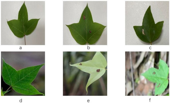
Figure 1.
Example Image of Lesion. (a) Images of healthy maple leaves in simple scenes. (b) Images of maple leaf spot disease in simple scenes. (c)Images of maple brown spot disease in simple scenes. (d) Images of healthy maple leaves in real scenes. (e) Images of maple leaf spot disease in real scenes. (f) Images of maple brown spot disease in real scenes.
Figure 1 displays representative images of maple leaves from six categories in the dataset. Portions (a) and (d) depict healthy leaf images of maples in simple and real scenarios, respectively. Portions (b) and (e) represent leaf spot disease images of maples in simple and real scenarios, while (c) and (f) represent leaf spot disease images of maples in simple and real scenarios, respectively.
According to Table 1, there are significant differences in the number of original images for the six types of images. Since the captured image data only include a single leaf, the number of image data that meets the requirements also varies. However, in order to improve the segmentation accuracy of lesions, this article adopts data augmentation technology to mitigate the negative impact on the model performance caused by category differences. At the same time, in order to accurately determine the accuracy of the grading, all image data have been subjected to disease grading.

Table 1.
Number of Images of Each Type of Lesion.
Labelling of the leaf and diseased spot locations was handled precisely with the LabelMe program. The original image and the labelled images produced after labelling are shown in Figure 2 and Figure 3, respectively. In Figure 2, the maple tree’s leaf area and the area affected by the leaf spot disease are depicted in red and green, respectively, while in Figure 3, the leaf area and the area affected by the leaf spot disease are depicted in red and yellow, respectively.
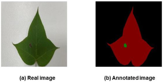
Figure 2.
Labeling of Leaf Spot Disease Images.
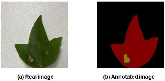
Figure 3.
Image Annotation of Brown Spot Disease.
2.1.2. Data Preprocessing
Adopting effective preprocessing techniques can not only accelerate the training process of convolutional neural networks but also help improve the segmentation accuracy and generalization ability of the model. Given that the input feature range of the CNN algorithm is extremely wide, exceeding its acceptable range will affect the accuracy of the algorithm [23]. Therefore, this article adopts a normalization method to accelerate the accuracy of the CNN algorithm and better capture the differences between images. The normalization method in this article is as follows: normalize the data by subtracting the channel mean and dividing it by the channel standard deviation, with all pixel values within the range of [–1, 1] [24].
To better apply the CNN model, this paper uses data enhancement technology to simulate the environmental conditions when photographing Liquidambar formosana leaves. This technique effectively reduces the risk of overfitting. By using three techniques: angle interference, light interference, and noise interference, the dataset’s capacity is increased. Some examples of enhanced datasets are shown in Figure 4.
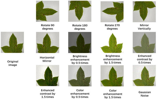
Figure 4.
Examples of Partial Data Enhancement Processing.
In real-world situations, fresh images can be added to the model continuously, considerably enhancing the model’s generalization performance by utilizing ImageDataGenerator to input training sets into the model and modifying the associated parameters to rotate and deform the images.
2.1.3. Dataset Partitioning
In this study, the SLSD dataset, which contains 1010 images, was used for all convolutional neural network training and testing. The training, verification, and test datasets for the SLSD algorithm are all included. Different uses are made of these three databases. The network model is trained using the training dataset, verified using the verification dataset to fine-tune the network model’s hyperparameters, and tested using the test dataset to see how well the network model generalizes.
It is crucial to make sure that all three datasets have both simple background images and complicated background images in order to separate the datasets based on the lesion category. The following steps are involved in the division process:
First, training datasets, validation datasets, and test datasets are created from the original photos in the following ratio: 6:2:2.
Secondly, only the training dataset is increased, leaving the other two types of datasets untouched. The data augmentation methods described in Section 2.1.2 are utilized for network training.
Thirdly, the performance of the segmentation network was assessed using the average of the findings from five experiments. There are 7878, 202, and 202 photos in the training set, validation set, and test set, respectively.
2.2. Improved DeepLabV3+ Semantic Segmentation Algorithm for Sweetgum Leaf Lesions
The DeepLabV3+ model performs well on the SLSD dataset, but there are still some challenges to overcome. Firstly, in order to achieve higher segmentation accuracy, a Modified Aligned Xception network with a large number of parameters was selected as the backbone feature extraction network for the encoder part. This increased the difficulty of network training and resulted in a decrease in network training speed and slow convergence. Additionally, as the spatial dimension of the input data continues to shrink, valuable feature information may be omitted during the feature extraction process of the encoder. Furthermore, direct input of shallow network information into the decoder will result in poor patch segmentation performance. By redesigning the DeepLabV3+ model, its segmentation performance can be significantly optimized, and its original shortcomings can be overcome.
To improve the segmentation performance of the model and address the aforementioned shortcomings, this article made the following improvements to the traditional DeepLabV3+ model structure:
- Replacing it with a lightweight MobileNetV2 network, which is much smaller than the original. This can effectively save resources and significantly accelerate the calculation speed of the model.
- Introducing SANet behind the backbone feature extraction network to solve the problem of precision decline caused by replacing the backbone network. This helps in training a better segmentation model.
- Introducing the CBAM-FF module to the decoder to improve the segmentation effect of the model on lesions and enhance segmentation accuracy.
The HAB-DeepLabV3+ network structure proposed in this article is shown in Figure 5.
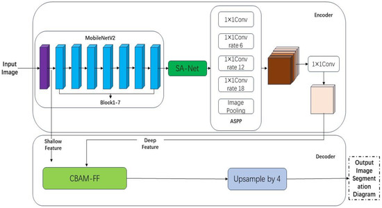
Figure 5.
HAB-DeepLabV3+ Network Architecture.
2.3. CBAM-FF Feature Fusion Module
CBAM [25] starts with two scopes: channel and spatial. It introduces spatial attention and channel attention as two analytical dimensions to achieve a sequential attention structure from channel to space. The spatial attention module (SAM) enables neural networks to focus more on the pixel regions in the image that play a decisive role in disease segmentation, while ignoring irrelevant regions. The channel attention module (CAM) is used to handle the allocation relationship of feature map channels. Simultaneously, the allocation of attention to these two dimensions enhances the performance improvement effect of the attention mechanism on the model. The CBAM structure is shown in Figure 6.
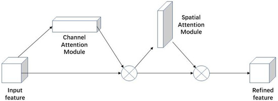
Figure 6.
CBAM Structure Diagram [25]. The module has two sequential sub-modules: channel and spatial. The intermediate feature map is adaptively refined through the module (CBAM) at every convolutional block of deep networks.
The classic DeepLabV3+ network directly fuses the shallow feature layer with the deep feature layer of quadruple upsampling during segmentation, without considering the problem of feature alignment at different levels. Convolutional neural networks expand the perception range by downsampling feature maps, thereby reducing the resolution of deep features and affecting the accurate positioning of targets. However, they can still provide strong semantic information, while shallow features have rich spatial information but a low semantic level. Due to the different content of the two types of information, directly fusing them together may lead to semantic inconsistency. Therefore, this article introduces CBAM-FF, which can fuse features from different levels and perceptual ranges. By assigning different weight coefficients to the feature map, we can extract important features related to disease spot information, suppressing the complex background, and improving the network robustness of this paper. As shown in Figure 7, the feature fusion module based on CBAM (referred to as CBAM-FF hereinafter) is constructed.
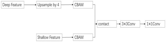
Figure 7.
Feature Fusion Module.
As shown in Figure 8, the channel attention mechanism extracts spatial information from features through MaxPool and AvgPool. It generates the sum of two spatial context features, and then inputs these two features into a network composed of a multilayer perceptron (MLP) with a hidden layer for operation and addition. Finally, it obtains the channel attention M_C through the sigmoid function operation. The specific calculation is shown in Equation (1).
where: represents the activation function, W0 RC/r C, and W1 RC C/r. Note that the MLP weights W0 and W1 are shared for the two inputs, and the ReLU activation function is applied after W0.
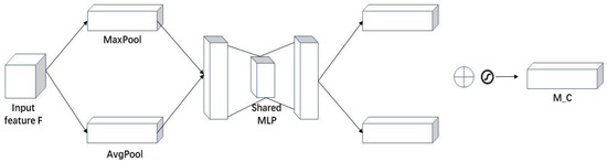
Figure 8.
Structure diagram of CAM. The channel sub-module utilizes both max-pooling outputs and average-pooling outputs with a shared network.
Spatial attention, as a supplement to channel attention, focuses on the positional information within the same channel. As shown in Figure 9, the spatial attention input feature F1 = C H W is averaged and maximally pooled to obtain F1avg = 1 H W and F1max = 1 H W. These results are then concatenated based on channels to obtain a feature map of F1avg+max= 2 H W. The spatial attention matrix M is obtained through a sigmoid function operation, denoted by M_S.
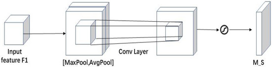
Figure 9.
SAM Structure Diagram. The spatial sub-module utilizes similar two outputs that are pooled along the channel axis and forward them to a convolution layer.
The calculation is shown in (2).
where: represents the activation function, and represents the convolution operation with a filter size of 7 7.
2.4. Backbone Feature Extraction Network
The research on lightweight deep learning neural networks has extremely important value, as lightweight models can save computer resources and overcome storage limitations. The lightweight neural network MobileNetV2 replaces the original backbone network of the modified aligned Xception model to achieve lightweight segmentation for the leaf spot model.
MobileNet is a lightweight deep neural network proposed by Google for embedded devices such as smartphones. MobileNetV2 [26] is an upgraded version of MobileNetV1 [27], typically activated by a ReLU after convolution. In MobileNetV1, ReLU6 is used, with a maximum output limit of 6. However, MobileNetV2 has removed the final output ReLU6 and directly outputs linearly. The reverse residual structure of the MobileNetV2 network consists of three parts. Firstly, it employs 1 1 convolutions to increase the dimensionality of input features, followed by 3 3 depth separable convolutions (DSC) for feature extraction, and then uses 1 1 convolutions for size reduction. Assuming the input feature map is m n 16 and the desired output is 32 channels, the convolutional kernel should be 16 3 3 32. It can be decomposed into a depth convolution, resulting in a feature map of 16 channels, followed by a point-by-point convolution to obtain the final output feature map. If standard convolution is used, the computational cost is m × n × 16 × 3 × 3 × 32 = m × n × 4608, while with DSC, the computational cost is m × n × 16 × 3 × 3 + m × n × 16 × 1 × 1 × 32 = m × n × 656. Compared to traditional convolution methods, deep separable convolution can significantly reduce computational complexity.
Unlike the previous narrow and fat residual structure, MobileNetV2 utilizes an inverted residual structure. As shown in Figure 10 below, a point-by-point convolution is used to expand the number of channels before the depth convolution to reduce feature loss, and the ReLU6 activation function is applied between convolutions. Finally, another point-by-point convolution is used to reduce dimensionality, enabling it to match the number of channels in the shortcut connection. To address the issue of useful information loss at low latitudes in ReLU6, the linear activation function is used as a replacement. The structural parameters of MobileNetV2 are presented in Table 2, where “t” represents the expansion factor, “C” denotes the depth of the output feature matrix, “N” signifies the number of Bottleneck repetitions (referring to the inverted residual structure), and “S” represents the stride distance.
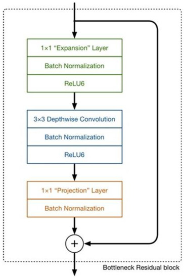
Figure 10.
Main Components of MobileNetV2.
Table 2.
MobileNetV2 Structure Parameter Table.
2.5. SANet Attention Mechanism
In order to address the problem of decreased segmentation accuracy caused by the lightweight improvement of the model, this paper introduces SANet in the backbone feature extraction network section. SANet [28] integrates feature space domain and channel domain information through the ShuffleAttention (SA) module, and SANet is divided into three parts: feature grouping, mixed attention mechanism, and feature aggregation. The specific structure is shown in Figure 11.
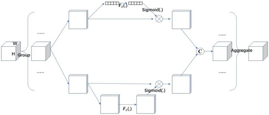
Figure 11.
SANet Structure Diagram [28].
Firstly, in the feature grouping section, SANet divides the input feature map X into multiple sub-features along the channel dimension. Then, in the mixed attention mechanism section, each sub-feature is divided into two parallel branches to learn attention features in the channel domain and spatial domain, respectively. Finally, in the feature aggregation section, each sub-feature is aggregated to obtain a feature map with spatial and channel domain information. SANet uses “channel segmentation” to process each group of sub-features in parallel. For the channel attention branches, GAP is used to generate channel statistics, and then a pair of parameters is used to scale and shift the channel vector. For the spatial attention branches, group norms are used to generate spatial statistical information, and then a compact feature of the channel branches is created. These two branches are then connected together. Finally, “channel shuffle” is used to achieve information exchange between different sub-features.
2.6. Optimization of Loss Function
The same sort of illness spots have varying sizes and shapes according to the SLSD dataset. These spots present a problem in the semantic segmentation task of maple leaf disease spots, and using the cross-entropy loss function can improve the model’s precision in identifying the disease spot area. As a result, the focal loss is developed to improve the segmentation accuracy of the model for illness spots by optimizing the loss function by including weight components. In Formula (3), the precise shape of the focal loss is displayed.
In Formula (3), is a simple/difficult regulatory factor, and is also the focusing parameter. When the t of is close to 0, it indicates that there is inaccurate category prediction, while is approaching 1. Here and are 2 and 0.25, respectively.
2.7. Evaluation Indicators
The evaluation indicators used in the experimental study are mean intersection over union (MIoU), pixel accuracy (PA), and mean pixel accuracy (MPA).
In the study of semantic segmentation, the intersection and union ratio represents the ratio of the intersection and union of the true labels and predicted values for each class. MIoU is a method used to measure the average intersection and union ratio for each category in a dataset. It calculates the ratio of the true value and predicted value for each category and combines these categories to obtain the average value for each category. The calculation formula is shown in Equation (4).
PA is an indicator used to measure the accuracy of predictions, which can be calculated using Formula (5).
With the aid of MPA, it is possible to determine the percentage of pixels that belong to each category’s accurate grouping, as well as the average of all properly organized categories. In (6), the computation formula is displayed.
Among them, is the total number of categories. Pij represents the number of pixels that originally belonged to class i but were predicted as class j. Pii represents the number of correctly predicted pixels, while Pij and Pji represent false positives and false negatives, respectively.
3. Results
3.1. Experimental Setup
- Experimental Platform Configuration
The platform settings for this experiment are shown in Table 3.
Table 3.
Experimental Platform Configuration.
- 2.
- Experimental Hyperparameter Setting
In order to improve the generalization performance and convergence speed of the model, the pre-training parameters of the backbone network on ImageNet were used. During model training, the image input size is 256 256, and the epoch is adjusted to 50 to better identify more features. Select the best hyperparameter combination and the best optimization algorithm. Select Adam for all model optimizations, adjust the initial value of loss to 0.001, and perform real-time detection on the epoch. If there are no significant fluctuations in the loss data, adjust the learning efficiency of the optimizer to 50%.
3.2. The Experimental Process
Based on the findings presented in Table 4, it becomes evident that the selection of hyperparameter combinations significantly affects the segmentation performance of the DeepLabV3+ network in maple leaf spot segmentation tasks.
Table 4.
Comparison of hyperparameter Performance of DeepLabV3+ Network.
Nonetheless, the overall performance of multiple hyperparameter combinations remains consistently excellent, with minimal variation. This observation indicates the remarkable stability of the DeepLabV3+ network when addressing maple leaf spot segmentation. Notably, the optimal segmentation performance is achieved when the learning rate is set to 0.0001, accompanied by Adam batch size values of 16.
Figure 12 and Figure 13 show the training results of the DeepLabV3+ network model and the proposed liquidambar leaf disease spot model HAB-DeeplabV3+. The red is the DeepLabV3+ network training process, and the gray is the HAB-DeeplabV3+ network training process. When the DeepLabV3+ network is iterated more than 70 times, the loss value also fluctuates significantly. When the number of iterations of the HAB-DeeplabV3+ network exceeds 70 times, the loss value has become stable, and the accuracy increases with the increase of iterations, and finally gradually stabilizes.
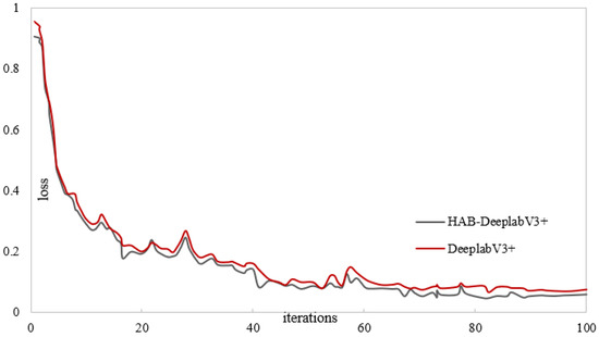
Figure 12.
Loss value change curve.
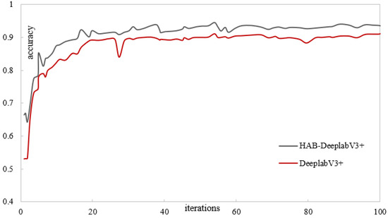
Figure 13.
Accuracy value change curve 3.3. Comparative experiments on the segmentation accuracy of models for different lesions.
The training process of the network first undergoes a freeze training operation (i.e., only the decoding layer participates in the training), maintaining the encoding layer’s unchanged parameters during feature extraction. Finally, a comprehensive training operation is carried out, with both the decoding layer and the encoding layer participating in the training. If the loss value of the training set does not change within 10 epochs, the training early stop operation is executed, that is, the training network is stopped.
To compare the segmentation performance of the HAB-DeeplabV3+model proposed in this article for maple leaf disease in different backgrounds, the best performing model was selected from the five obtained models for analysis. Table 5 compares DeeplabV3+ and HAB DeeplabV3+ in the four categories of PA and IoU in the dataset used. From the table, it can be seen that compared with DeeplabV3+, HAB DeeplabV3+has a 6.8% increase in PA and 12.1% increase in IoU for leaf spot segmentation under complex backgrounds, and a 7.7% increase in PA and 8.7% increase in IoU for brown spot segmentation under real complex backgrounds. It is more pronounced for the improvement of lesions under two simple backgrounds.
Table 5.
Comparison of segmentation accuracy of lesions.
3.3. Disease Grading Detection Based on Pixel Statistics
3.3.1. Classification and Detection Methods for Lesions
Due to the lack of a clear grading standard for the degree of leaf spot disease in maple leaves, in order to more accurately analyze the degree of leaf spot disease in maple leaves, this article referred to the <<Classification Standard for Corn Brown Spot Disease>> (DB13/T 1732-2013) formulated in accordance with GB/T 1.1-2019 to develop a grading parameter standard for maple leaf spot disease. This article is based on the principle of pixel statistics and uses Python to achieve the statistics of the lesion area. The leaves are divided into four levels, namely: healthy leaves, Level 1, Level 2, and Level 3. The criteria for grading leaf lesions are shown in Table 6.
Table 6.
Classification of Maple Leaf Disease Spots.
Where k is the proportion of the lesion area to the entire image, and its principal calculation formula is shown in (7).
In the formula, Ascab represents the area of the lesion area, Aimage represents the area of the entire leaf, Rscab represents the lesion area, and Rimage represents a partial area of the leaf.
3.3.2. Comparative Experiment on Grading Detection
Based on the hierarchical leaf brown spot data set, this section has set up comparative experiments. The network models include the DeepLabV3+model with ResNet101 as the backbone network, the DeepLabV3+model with MobileNetV2 as the backbone network, CBAM-FF+DV3+, and HAB-DeepLabV3+. The experimental results of the models’ identification accuracy for different grades of lesions are shown in Table 7. The CBAM-FF+DV3+ in the table represents the introduction of the CBAM-FF module into the DeeplabV3+ network model, and HAB DeepLabv3+ is the method proposed in this article.
Table 7.
Comparison of Accuracy of Different Models.
From Table 7, it can be seen that all models in the experiment have the highest recognition accuracy for healthy leaves and Level 1 categories because healthy leaves do not contain diseased spots or have small diseased spot areas, resulting in low segmentation accuracy and high recognition accuracy. As shown in Figure 14, the comparison of the segmentation accuracy of each model for graded lesions is shown.
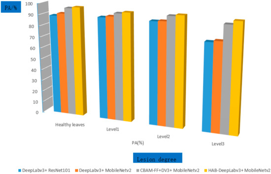
Figure 14.
Comparison of Model Accuracy.
It can be more clearly seen from Figure 14 and Table 7 that the HAB DeeplabV3+ proposed in this article has improved the accuracy for healthy leaves and Level 1 by 1.1% and 1.2%, respectively, compared to DeeplabV3+, CBAM-FF+DeeplabV3+ and has also improved the accuracy for Level 2 and Level 3. Overall, the HAB-DeeplabV3+ proposed in this article has the best recognition accuracy for healthy leaves, Level 1, Level 2, and Level 3.
4. Discussion
4.1. Comparative Experiment on Different Placement Positions of Modules
In order to evaluate the performance of the proposed CBAM-FF feature fusion module in the maple leaf spot segmentation task, the SLSD dataset was used to conduct experiments in the DeepLabV3+ segmentation network with modified aligned Xception as the backbone network. Using the same dataset partitioning method, each network only undergoes one training and model testing. Experimental comparisons were conducted on the placement positions of CBAM, CBAM-FF, and other two modules in the decoder. The experimental software and hardware configurations remain consistent with those outlined in Section 3.3.2.
Within the decoder, two distinct positions exist for module placement. The first position corresponds to the output location of the DCNN in the decoder, while the second position represents the entry point where the DCNN output enters the decoder through parallel hole convolution. CBAM-FF module adds the attention mechanism in two positions at the same time, and the experiment verifies the performance of the CBAM-FF module by adding the attention mechanism to different positions. The conducted experiments are as follows:
Experiment 1: CBAM is placed in position 1.
Experiment 2: CBAM is placed in position 2.
Experiment 3: A CBAM-FF module is added to the decoder.
The impact of modules on segmentation performance is shown in Table 8.
Table 8.
Impact of modules on segmentation performance.
From Table 8, it can be seen that when CBAM is placed at the output position of DCNN in the decoder, MIoU increases by 1.3%, reaching 86.87%. When CBAM is placed at the position where DCNN output enters the decoder through parallel hole convolution, MIoU further increases to 86.61%. When the CBAM-FF module was introduced into the decoder, MIoU increased by 3.5% to 88.74%, while MPA also improved to some extent. Therefore, it can be concluded that adding CBAM-FF to the decoder can better enhance the MloU of the DeepLabV3+ network in the semantic segmentation task of maple leaf disease spots than simply introducing CBAM.
4.2. The Impact of SANet on Segmentation Performance
In order to verify the performance of the added SANet in the maple leaf spot segmentation task, the SLSD dataset was used to conduct experiments in the DeepLabV3+ segmentation network with MobileNetV2 as the backbone network. Using the same dataset partitioning method, each network only undergoes one training and model testing.
The ECANet [29], SENet [30], and SANet attention mechanisms are all plug and play modules. The SENet attention mechanism can focus on the weight of each channel for the input feature layer. ECANet is an improved version of SENet, which removes the fully connected layer from the previous generation and learns directly through convolution on the features after global average pooling. Each group of experiments placed attention mechanism modules at the same position as the encoder. Experiment 1 represented the DeeplabV3+ semantic segmentation network with the CBAM-FF module added, Experiment 2 represented ECANet placement, Experiment 3 represented SENet placement, and Experiment 4 represented SANet placement. Comparative experiments were conducted on the three attention mechanism modules, and the experimental results are shown in Table 9.
Table 9.
Comparison of experimental results for inserting various modules.
From Table 9, it can be seen that when adding the ECANet module to the encoder, the MIoU increased by 0.9% to 88.37%. When adding the SENet module to the encoder, the MIoU increased by 0.8%. When adding the SANet module to the encoder, the MIoU increased by 1.8% to 89.16%. This indicates that SANet has better performance and higher segmentation accuracy compared to other attention modules.
4.3. Ablation Experiment
The effectiveness of replacing backbone networks, CBAM-FF, and SANet can be evaluated by setting four sets of ablation experiments on the SLSD dataset. Train each group of networks only once and simulate and evaluate their results. Set the batch size and epoch to 16 and 0.0001, respectively, and epoch to 50. At the same time, real-time checks will be conducted on the loss. If there are no changes to the loss values in the two epochs, adjust them to 50%. Experimental comparisons were conducted on the placement positions of CBAM, CBAM-FF, and other two modules in the decoder. The experimental results are shown in Table 10.
Table 10.
Results of ablation experiment.
Experiment 1: Based on the classic Deeplab 3+ network structure, replace the backbone feature extraction network with a MobileNetV2 network;
Experiment 2: Based on Experiment 1, introduce SANet after the backbone feature network;
Experiment 3: On the basis of Experiment 2, add a CBAM-FF module to the decoder section;
Experiment 4: Add focal loss function on the basis of Experiment 3.
According to the results of the ablation experiment, the model size of Experiment 1 reached 25.7 M, indicating the effectiveness of replacing the classic DeeplabV3+ backbone feature extraction network with MobileNetV2. Experiment 2 and Experiment 3 have improved the MPA and MIou of the classic DeeplabV3+, while Experiment 2 has improved the MPA and MIou by 1.3% and 1.9%, respectively. Adding SANet not only improves the accuracy of the model, but also has no impact on the size of the model. The MPA and MIou of Experiment 3 increased by 2.3% and 3.2%, respectively, indicating that the addition of CBAM-FF module significantly improved the segmentation accuracy of the network model. From the results of Experiment 4, the optimization of loss function improves the segmentation accuracy of the model for the diseased area and effectively solves the problem of low segmentation accuracy caused by the imbalance of data samples in the network training process.
4.4. Comparison of Different Segmentation Methods
In order to further verify the segmentation performance of the HAB DeeplabV3+model, the method in this paper is compared with the semantic segmentation models commonly used for plant disease such as the classic DeeplabV3+ [31], U-Net [32], SegNet [33], SEMD [34], and the comparison results are shown in Table 11. From Table 5 and Table 11, it can be seen that the model proposed in this paper has the best accuracy in lesion segmentation.
Table 11.
Comparison of evaluation indicators for different segmentation models.
According to the experimental results in Table 11, the MPA of HAB DeeplabV3+is 94.75%, which is 3.4% higher than the classic DeeplabV3+. The MIoU of the algorithm proposed in this article is 90.23%, which is an improvement of 4.55% compared to the classic DeeplabV3+. In terms of parameter quantity, the HAB DeeplabV3+ in this article reduces 27.75 M, 6.75 M, and 11.75 M compared to DeeplabV3+, U-Net, and SegNet, respectively.
The experimental data show that replacing MobilenetV2 in this article reduces the number of parameters in the model and achieves lightweighting of the model. This article introduces the CBAM-FF module and SANet, respectively, which change the expression of features and enhance their expression ability.
This article also visualized the segmentation effects of the four algorithms, as shown in Figure 15. From the comparison, it can be seen that the classic DeeplabV3+ and HAB-DeeplabV3+ have higher recognition accuracy for the edge of diseased areas compared to U-Net and SegNet. Due to the fact that DeeplabV3+ contains different rates of Atrous Convolution in the encoding section for feature extraction, it can enhance the recognition ability for objects of different sizes and have the ability to recover the feature information of the area edge. Compared with the classic DeeplabV3+, HAB-DeeplabV3+ has improved edge recognition of lesion areas. Compared with U-Net and SegNet, it has better segmentation performance for lesion areas. This proves that adding the CBAM-FF module and SANet can enhance the ability to extract lesion areas and edge information features.
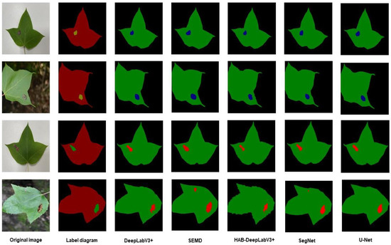
Figure 15.
Comparison of segmentation effects.
5. Conclusions
In this study, we proposed an improved disease spot segmentation method based on the DeeplabV3+ network. Our approach introduced a CBAM-FF feature fusion module and an attention mechanism in the backbone feature extraction network and decoder parts, respectively, to enhance the model’s feature extraction capability. We also employed the focal loss function to improve the segmentation accuracy of the model for lesion areas by emphasizing the learning of lesion samples. Additionally, we replaced the modified aligned Xception network used for backbone feature extraction with a MobileNetV2 network to reduce the computational complexity of the model’s parameters.
Experimental evaluations were conducted on the SLSD dataset, and the results demonstrated the effectiveness of our proposed HAB DeeplabV3+ network model. Compared to the classic DeeplabV3+ model, our model achieved a notable improvement with a 3.4% increase in mean pixel accuracy (MPA), a 4.55% increase in mean intersection over union (MIoU), and a reduction of 27.75 M model parameters. These results indicate that our method can effectively segment the diseased areas of maple leaves.
However, it should be noted that the segmentation performance on other plant leaf lesion images remains unknown. In future work, we plan to conduct pre-training on other plant leaf lesion datasets to achieve segmentation and detection of different lesions in real environments. By further expanding the scope of our approach, we aim to provide a comprehensive solution for detecting and segmenting various plant leaf diseases.
Author Contributions
Methodology, P.W.; Resources, G.W. and L.M.; Data curation, C.K.; Writing—original draft, M.C. (Maodong Cai); Writing—review & editing, P.W. and M.C. (Musenge Chola); Project administration, X.Y.; Funding acquisition, L.M. All authors have read and agreed to the published version of the manuscript.
Funding
This research received no external funding.
Data Availability Statement
Not available.
Conflicts of Interest
The authors declare no conflict of interest.
References
- Liu, D.; Yang, H.; Gong, Y.; Chen, Q. A Recognition Method of Crop Diseases and Insect Pests Based on Transfer Learning and Convolution Neural Network. Math. Probl. Eng. 2022, 2022, 1470541. [Google Scholar] [CrossRef]
- Khakimov, A.; Salakhutdinov, I.; Omolikov, A.; Utaganov, S. Traditional and current-prospective methods of agricultural plant diseases detection: A review. IOP Conf. Ser. Earth Environ. Sci. 2022, 951, 012002. [Google Scholar] [CrossRef]
- Li, Y.; Wan, Y.; Lin, W.; Ernstsons, A.; Gao, L. Estimating Potential Distribution of Sweetgum Pest Acanthotomicus suncei and Potential Economic Losses in Nursery Stock and Urban Areas in China. Insects 2021, 12, 155. [Google Scholar] [CrossRef] [PubMed]
- Mao, Y.; Zheng, X.; Chen, F. First report of leaf spot disease caused by Corynespora cassiicola on American sweetgum (Liquidambar styraciflua L.) in China. Plant Dis. 2021; Online ahead of print. [Google Scholar]
- Mallikarjuna, P.B.; Guru, D.S. Fusion of Texture Features and SBS Method for Classification of Tobacco Leaves for Automatic Harvesting. Lect. Notes Electr. Eng. 2013, 213, 115–126. [Google Scholar]
- Ma, J.; Du, K.; Zhang, L.; Zheng, F.; Chu, J.; Sun, Z. A segmentation method for greenhouse vegetable foliar disease spots images using color information and region growing. Comput. Electron. Agric. 2017, 142 Pt 1, 110–117. [Google Scholar] [CrossRef]
- Pan, T.-t.; Chyngyz, E.; Sun, D.-W.; Paliwal, J.; Pu, H. Pathogenetic process monitoring and early detection of pear black spot disease caused by Alternaria alternata using hyperspectral imaging. Postharvest Biol. Technol. 2019, 154, 96–104. [Google Scholar] [CrossRef]
- Appeltans, S.; Pieters, J.G.; Mouazen, A.M. Detection of leek white tip disease under field conditions using hyperspectral proximal sensing and supervised machine learning. Comput. Electron. Agric. 2021, 190, 106453. [Google Scholar] [CrossRef]
- Singh, V. Sunflower leaf diseases detection using image segmentation based on particle swarm optimization. Artif. Intell. Agric. 2019, 3, 62–68. [Google Scholar] [CrossRef]
- Khan, K.; Khan, R.U.; Albattah, W.; Qamar, A.M. End-to-End Semantic Leaf Segmentation Framework for Plants Disease Classification. Complexity 2022, 2022, 1168700. [Google Scholar] [CrossRef]
- Wspanialy, P. A detection and severity estimation system for generic diseases of tomato greenhouse plants. Comput. Electron. Agric. 2020, 178, 105701. [Google Scholar] [CrossRef]
- Bhagat, S.; Kokare, M.; Haswani, V.; Hambarde, P.; Kamble, R. Eff-UNet++: A novel architecture for plant leaf segmentation and counting. Ecol. Inform. Int. J. Ecoinform. Comput. Ecol. 2022, 68, 101583. [Google Scholar] [CrossRef]
- Wei, F.; Li, W.; Ma, B.; Yan, Z.; Zhi, W.; Zhang, L.; Xian, D.; He, Y.; Deng, X.; Chen, Y.; et al. Local CRF and oxytocin receptors correlate with female experience-driven avoidance change and hippocampal neuronal plasticity. Neurochem. Int. 2023, 163, 105485. [Google Scholar] [CrossRef] [PubMed]
- Warjri, S.; Pakray, P.; Lyngdoh, S.A.; Maji, A.K. Part-of-speech (POS) tagging using conditional random field (CRF) model for Khasi corpora. Int. J. Speech Technol. 2021, 24, 853–864. [Google Scholar] [CrossRef]
- Lin, B.; Fan, X.; Guo, Z. Self-attention module in a multi-scale improved U-net (SAM-MIU-net) motivating high-performance polarization scattering imaging. Opt. Express 2023, 31, 3046–3058. [Google Scholar] [CrossRef]
- Wang, Z.; Li, J.; Song, G.; Li, T. Faster Speed: Refining Self-Attention Module for Image Reconstruction. arXiv 2019, arXiv:1905.08008. [Google Scholar]
- Shang, J.; Wang, J.; Liu, S.; Wang, C.; Zheng, B. Small Target Detection Algorithm for UAV Aerial Photography Based on Improved YOLOv5s. Electronics 2023, 12, 2434. [Google Scholar] [CrossRef]
- Li, R.; Wang, L.; Zhang, C.; Duan, C. A2-FPN for semantic segmentation of fine-resolution remotely sensed images. Int. J. Remote Sens. 2022, 43, 1131–1155. [Google Scholar] [CrossRef]
- Wan, W.; Luo, X.; Ma, L.; Xie, S. Side-path FPN-based multi-scale object detection. Int. J. Comput. Sci. Eng. 2022, 25, 1. [Google Scholar] [CrossRef]
- Cai, F.; Hu, Q.; Zhou, R.; Xiong, N. REEGAT: RoBERTa Entity Embedding and Graph Attention Networks Enhanced Sentence Representation for Relation Extraction. Electronics 2023, 12, 2429. [Google Scholar] [CrossRef]
- Gong, Y.; Wang, F.; Lv, Y.; Liu, C.; Li, T. Automatic Sleep Staging Using BiRNN with Data Augmentation and Label Redirection. Electronics 2023, 12, 2394. [Google Scholar] [CrossRef]
- Aboussaleh, I.; Riffi, J.; Fazazy, K.E.; Mahraz, M.A.; Tairi, H. Efficient U-Net Architecture with Multiple Encoders and Attention Mechanism Decoders for Brain Tumor Segmentation. Diagnostics 2023, 13, 872. [Google Scholar] [CrossRef] [PubMed]
- Zamani Joharestani, M.; Cao, C.; Ni, X.; Bashir, B.; Talebiesfandarani, S. PM2.5 Prediction Based on Random Forest, XGBoost, and Deep Learning Using Multisource Remote Sensing Data. Atmosphere 2019, 10, 373. [Google Scholar] [CrossRef]
- Nagasubramanian, K.; Jones, S.; Singh, A.K.; Sarkar, S.; Singh, A. Plant disease identification using explainable 3D deep learning on hyperspectral images. Plant Methods 2019, 15, 98. [Google Scholar] [CrossRef] [PubMed]
- Woo, S.; Park, J.; Lee, J.-Y.; Kweon, I.S. CBAM: Convolutional Block Attention Module; European Conference on Computer Vision; Springer: Cham, Switzerland, 2018. [Google Scholar]
- Sandler, M.; Howard, A.; Zhu, M.; Zhmoginov, A.; Chen, L.-C. MobileNetV2: Inverted Residuals and Linear Bottlenecks. In Proceedings of the 2018 IEEE/CVF Conference on Computer Vision and Pattern Recognition (CVPR), Salt Lake City, UT, USA, 18–23 June 2018. [Google Scholar]
- Howard, A.G.; Zhu, M.; Chen, B.; Kalenichenko, D.; Wang, W.; Weyand, T.; Andreetto, M.; Adam, H. MobileNets: Efficient Convolutional Neural Networks for Mobile Vision Applications. arXiv 2017, arXiv:1704.04861. [Google Scholar]
- Zhang, Q.-L.; Yang, Y.B. SA-Net: Shuffle Attention for Deep Convolutional Neural Networks. In Proceedings of the ICASSP 2021–2021 IEEE International Conference on Acoustics, Speech and Signal Processing (ICASSP), Toronto, ON, Canada, 6–11 June 2021. [Google Scholar]
- Wang, Q.; Wu, B.; Zhu, P.; Li, P.; Zuo, W.; Hu, Q. ECA-Net: Efficient Channel Attention for Deep Convolutional Neural Networks. In Proceedings of the 2020 IEEE/CVF Conference on Computer Vision and Pattern Recognition (CVPR), Seattle, WA, USA, 13–19 June 2020. [Google Scholar]
- Hu, J.; Shen, L.; Albanie, S.; Sun, G.; Wu, E. Squeeze-and-Excitation Networks. In IEEE Transactions on Pattern Analysis and Machine Intelligence; IEEE: New York, NY, USA, 2019. [Google Scholar]
- Chen, L.-C.; Zhu, Y.; Papandreou, G.; Schroff, F.; Adam, H. Encoder-Decoder with Atrous Separable Convolution for Semantic Image Segmentation; Springer: Cham, Switzerland, 2018. [Google Scholar]
- Ronneberger, O.; Fischer, P.; Brox, T. U-Net: Convolutional Networks for Biomedical Image Segmentation. In International Conference on Medical Image Computing and Computer-Assisted Intervention; Springer: Cham, Switzerland, 2015. [Google Scholar]
- Badrinarayanan, V. SegNet: A Deep Convolutional Encoder-Decoder Architecture for Image Segmentation. IEEE Trans. Pattern Anal. Mach. Intell. 2017, 39, 2481–2495. [Google Scholar]
- Shi, L.; Wang, G.; Mo, L.; Yi, X.; Wu, X.; Wu, P. Automatic Segmentation of Standing Trees from Forest Images Based on Deep Learning. Sensors 2022, 22, 6663. [Google Scholar] [CrossRef]


Disclaimer/Publisher’s Note: The statements, opinions and data contained in all publications are solely those of the individual author(s) and contributor(s) and not of MDPI and/or the editor(s). MDPI and/or the editor(s) disclaim responsibility for any injury to people or property resulting from any ideas, methods, instructions or products referred to in the content. |
© 2023 by the authors. Licensee MDPI, Basel, Switzerland. This article is an open access article distributed under the terms and conditions of the Creative Commons Attribution (CC BY) license (https://creativecommons.org/licenses/by/4.0/).