Article

ICSF: An Improved Cloth Simulation Filtering Algorithm for Airborne LiDAR Data Based on Morphological Operations

1
State Key Laboratory of Information Engineering in Surveying, Mapping and Remote Sensing, Wuhan University, Wuhan 430079, China
2
Key Laboratory of Mine Environmental Monitoring and Improving around Poyang Lake of Ministry of Natural Resources, East China University of Technology, Nanchang 330013, China
3
Wuhan Botanical Garden, Chinese Academy of Sciences, Wuhan 430074, China
4
School of Surveying and Geoinformation Engineering, East China University of Technology, Nanchang 330013, China
5
College of Resources and Environment, Xingtai University, Xingtai 054001, China
6
Xingtai Key Laboratory of Geo-Information and Remote Sensing Technology Application, Xingtai 054001, China
*
Author to whom correspondence should be addressed.
Forests 2023, 14(8), 1520; https://doi.org/10.3390/f14081520
Submission received: 20 June 2023 / Revised: 18 July 2023 / Accepted: 20 July 2023 / Published: 26 July 2023
(This article belongs to the Special Issue Application of Laser Scanning Technology in Forestry)

Abstract

:
Ground filtering is an essential step in airborne light detection and ranging (LiDAR) data processing in various applications. The cloth simulation filtering (CSF) algorithm has gained popularity because of its ease of use advantage. However, CSF has limitations in topographically and environmentally complex areas. Therefore, an improved CSF (ICSF) algorithm was developed in this study. ICSF uses morphological closing operations to initialize the cloth, and estimates the cloth rigidness for providing a more accurate reference terrain in various terrain characteristics. Moreover, terrain-adaptive height difference thresholds are developed for better filtering of airborne LiDAR point clouds. The performance of ICSF was assessed using International Society for Photogrammetry and Remote Sensing urban and rural samples and Open Topography forested samples. Results showed that ICSF can improve the filtering accuracy of CSF in the samples with various terrain and non-ground object characteristics, while maintaining the ease of use advantage of CSF. In urban and rural samples, ICSF obtained an average total error of 4.03% and outperformed another eight reference algorithms in terms of accuracy and robustness. In forested samples, ICSF produced more accuracy than the well-known filtering algorithms (including the maximum slope, progressive morphology, and cloth simulation filtering algorithms), and performed better with respect to the preservation of steep slopes and discontinuities and vegetation removal. Thus, the proposed algorithm can be used as an efficient tool for LiDAR data processing.

1. Introduction

Airborne light detection and ranging (LiDAR) can quickly and accurately acquire three-dimensional structural information of landscapes, and has been widely used in various fields [1,2], e.g., terrain mapping [3,4,5,6,7], city modeling [8,9,10,11,12] and forestry inventory [13,14,15,16,17]. In almost all applications, ground filtering, i.e., distinguishing ground points from non-ground points, is a necessary step in LiDAR data processing [18,19,20]. For example, ground filtering is necessary to eliminate terrain effects in forestry application, such as tree species classification [14], tree height measurement [15] and biomass estimation [17]. Consequently, different types of filtering algorithms have been proposed in the past three decades. However, developing a filtering algorithm that is effective and easy to use in various landscapes still remains a challenge [21,22,23,24,25,26,27].
Existing filtering algorithms can be classified into three categories, i.e., slope-, morphology- and surface-based methods [28,29,30,31,32,33,34,35,36,37,38,39,40,41,42,43,44,45,46,47,48]. Slope-based methods separate LiDAR point clouds into ground and non-ground points, based on the assumption that the terrain slope changes gradually in a neighborhood, while the changes between non-ground points (e.g., buildings and vegetation points) and ground points are large. Morphology-based methods remove non-ground points according to the height differences of the morphological surfaces before and after opening operations. Surface-based methods gradually construct reference terrain using an interpolation method (e.g., triangulated irregular network (TIN)), and then select ground points based on the height differences between the points and the reference terrain. Sithole and Vosselman [3] released a well-known benchmark dataset and compared the performance of eight filtering algorithms using the dataset. They concluded that surface-based methods can achieve better results, because the methods use more context information than other filtering algorithms [3,41,46,49]. Among surface-based methods, the cloth simulation filtering (CSF) algorithm developed in recent years has received extensive attention and application because of its ease of use and integration with several types of software, e.g., CloudCompare v2.11.3, Point Cloud Magic v2.0, and 3DF Zephyr v7.0 [27].
CSF simulates the physical process of cloth covering towards an inverted (upside-down) point cloud to construct reference terrain, and then separates the point cloud into ground points and non-ground points, based on the height differences between unclassified points and the reference terrain. Specifically, a piece of horizontal cloth is placed above an inverted point cloud. Then, the shape of the cloth is simulated by an external force operation followed by an internal force operation. The external force operation is designed to move the cloth towards the inverted point cloud. The internal force operation aims to restrict the movement of the cloth to prevent the cloth from covering non-ground objects. The process is performed iteratively until the shape of the cloth no longer changes, and the cloth is considered as the reference terrain. Finally, ground points are extracted by comparing the height differences between unclassified points and the reference terrain. CSF is easy to use because users only need to set one enumeration parameter, i.e., cloth rigidness. The cloth rigidness controls the strength of internal force, and is divided into three categories: high, medium and low rigidness. These settings are usually applied to the flat terrain, slopes and raised terrain, respectively [2,13,27].
However, CSF also has limitations. First, it is difficult for cloth to cover steep slopes, where accurate reference terrain cannot be obtained to distinguish ground points from non-ground points [26]. For example, cloth particle p still cannot collide with the point q on steep slopes until the end of the simulation (Figure 1a). Second, a single cloth rigidness is unreasonable, because multiple terrain features (i.e., flat terrain, slopes and raised terrain) are usually contained in a landscape (Figure 1b) [50]. Third, the points on rugged terrain are often misclassified when using a fixed height difference threshold, since terrain slopes are not considered [26,50].
To solve these problems, Yang et al. [50] partitioned a point cloud into multiple regions, where the richness of terrain features became lower relative to in the entire scene, and thus the negative impact of cloth rigidness was reduced. In addition, the reference terrain of steep slopes was constructed using a bidirectional cloth simulation method. Finally, ground points were extracted based on adaptive height difference thresholds, which were calculated using a weighted sum of the height differences of unclassified points and their neighboring points. Wan et al. [51] proposed a terrain relief index to automatically estimate the cloth rigidness applicable to a scene. These improved algorithms improve the filtering accuracy of CSF, but sacrifice its ease of use, due to the introduction of many additional parameters.
Therefore, we aimed to develop a new improved CSF (ICSF) algorithm. The proposed algorithm is expected to not only solve the three problems of CSF, but to also maintain its ease of use advantage. Compared with the classical CSF algorithm, the main contributions of ICSF are as follows:
(1)
The cloth is initialized by morphological closing operations. The initialized cloth can cover steep slopes, where an accurate reference terrain can be obtained for filtering LiDAR point clouds.
(2)
Cloth rigidness can be set to low rigidness, since only the reference terrain of raised terrain needs to be constructed after cloth initialization. This improves the adaptability of the filtering in the landscapes containing multiple terrain features.
(3)
Ground points and non-ground points are distinguished based on the terrain-adaptive height difference thresholds with the consideration of terrain slopes. This can improve filtering accuracy on rugged terrain.

2. Methods

The flowchart of ICSF is illustrated in Figure 2. First, the cloth is initialized using morphological closing operations. Second, a reference terrain is estimated using cloth simulation that does not require a cloth rigidness setting. Finally, ground points are extracted using terrain-adaptive height difference thresholds.

2.1. Cloth Initialization

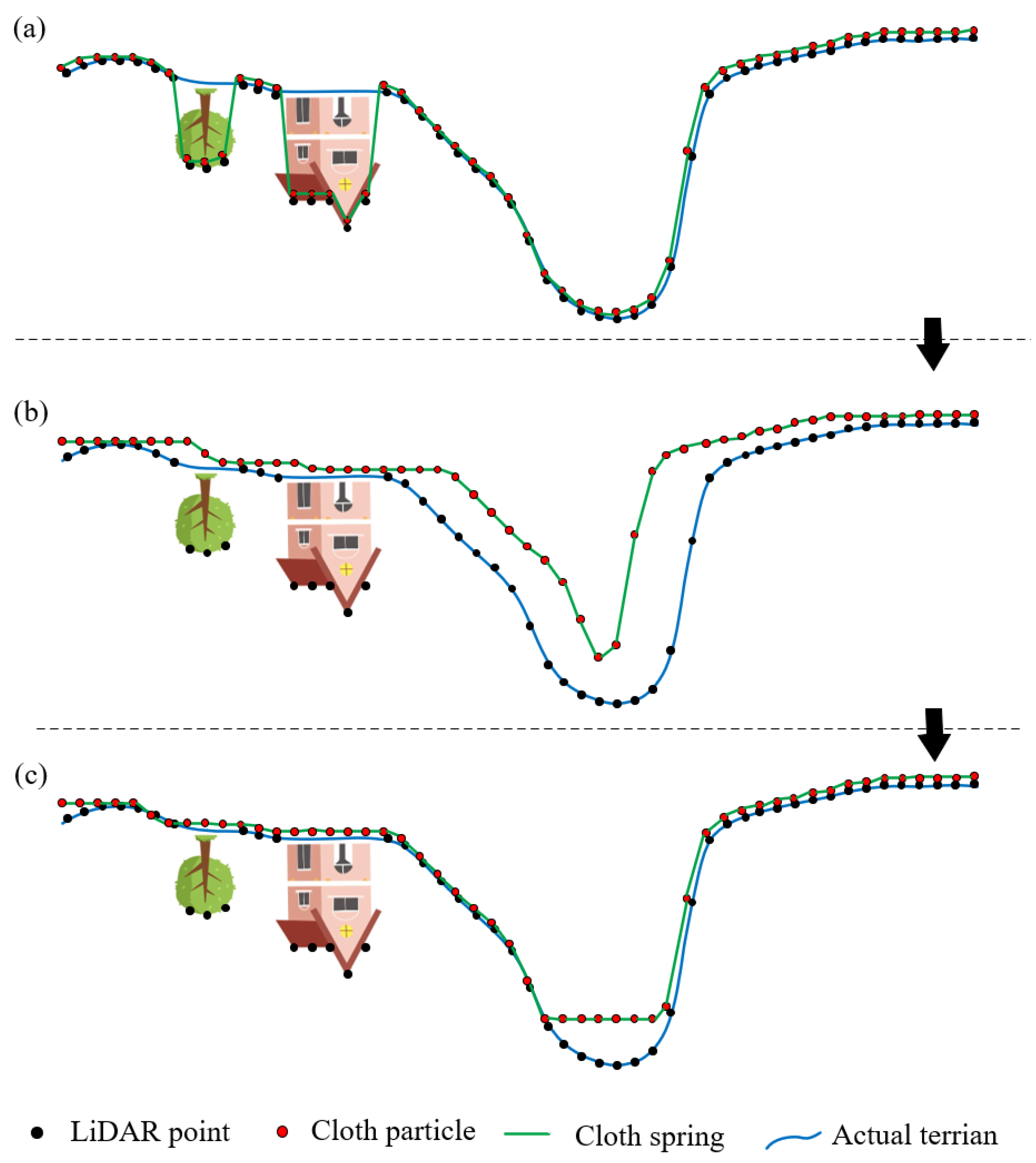
To overcome the limitation of cloth failing to cover steep slopes, we initialized the cloth using morphological closing operations. The cloth is modeled as a grid that consists of particles and springs based on the inverted point cloud. The particles are the center points of the cells in the grid, and particle values are the elevations of the highest points in the cells. The springs are established according to each particle and its eight neighboring particles (Figure 3a). Then, the cloth is initialized by morphological closing operations. The operation consists of a dilation operation D Cloth r ,   c followed by an erosion operation E Cloth r ,   c (Figure 3b,c). The two operations replace the value of a particle to the maximum and minimum values in a structuring element w, respectively [33,52]. They are expressed as:
D Cloth r ,   c = max ( r + u ,   c + v ) w ( Cloth   ( r + u ,   c + v ) ) E Cloth r ,   c = min ( r + u ,   c + v ) w ( Cloth   ( r + u ,   c + v ) )
where Cloth   ( r + u ,   c + v ) is the value of a particle within w. Note that the results of dilation operations are used as the inputs of erosion operations. The initialized cloth can cover not only flat terrain and gentle slopes, but also steep slopes (Figure 3c).

2.2. Reference Terrain Estimation

Only raised terrain in a landscape fails to be covered by cloth after initialization. The reference terrain is constructed using the cloth simulation with low rigidness. The cloth simulation consists of external force followed by internal force operations. Specifically, the value of a particle after an external force operation is defined in (2).
Cloth   ( r ,   c ) = Cloth   ( r ,   c ) s
where s represents the descending distance, which is set to 0.5 m [15]. After the external force operation, the collision detection between the particle and the point cloud is defined in (3).
δ = Cloth   ( r ,   c )   Point   ( r ,   c )
where δ represents the height difference between the cloth particle and the point cloud. Point   ( r ,   c ) is the height of the point cloud corresponding to the cloth particle. If δ is less than 0, it means that the cloth particle collides with the point cloud. The value of the cloth particle is adjusted by (4), and the property of the cloth particle is set to be unmovable.
Cloth   ( r ,   c ) = Cloth   ( r ,   c )   δ
The value of a cloth particle after the internal force operation is determined by traversing each spring of the particle. If the neighboring particle is unmovable, the value of the cloth particle is calculated by (5).
Cloth   ( r ,   c ) = Cloth   ( r ,   c ) + ( 1   1 2 ri )   ×   ( Cloth   ( r + u ,   c + v )   Cloth   ( r ,   c ) )
where ri is cloth rigidness, which is set to low rigidness, as mentioned above, i.e., ri is equal to 1. Otherwise, the cloth particle and the neighboring particle are moved in opposite directions to the same height. Note that the results of external force operations are used as the inputs of internal force operations. The simulation process is terminated if the maximum height change of all particles is small enough. The cloth after the simulation represents the reference terrain [27].

2.3. Ground Point Extraction

Ground points are extracted by comparing the height differences between unclassified points and the reference terrain. The height difference threshold is set according to local terrain slopes, and improving the adaptability of the filtering in the landscapes with rugged terrain. First, the terrain slope (θ) of each cloth particle is calculated by the following equation:
θ = a 2 + b 2 / | c |
where a, b and c are the parameters of the fitted plane (ax + by + cz + d = 0), which are constructed based on each particle and its eight neighbors using a least-squares plane fitting method. Then, the height difference thresholds from an unclassified point to its nine nearest-neighbor particles are calculated by the following equation:
H i = ε + θ   ×   d
where H i ( i = 1 ,   2 , ,   9 ) represents the height difference threshold corresponding to nine particles. d is the horizontal distance between the unclassified point and a particle. ε is the height residual, which is set to 0.2 m [53]. Finally, if the height differences between more than half of the particles and the unclassified point are less than the corresponding thresholds, the unclassified point is marked as a ground point.

3. Experiment Design and Accuracy Assessment

3.1. Data

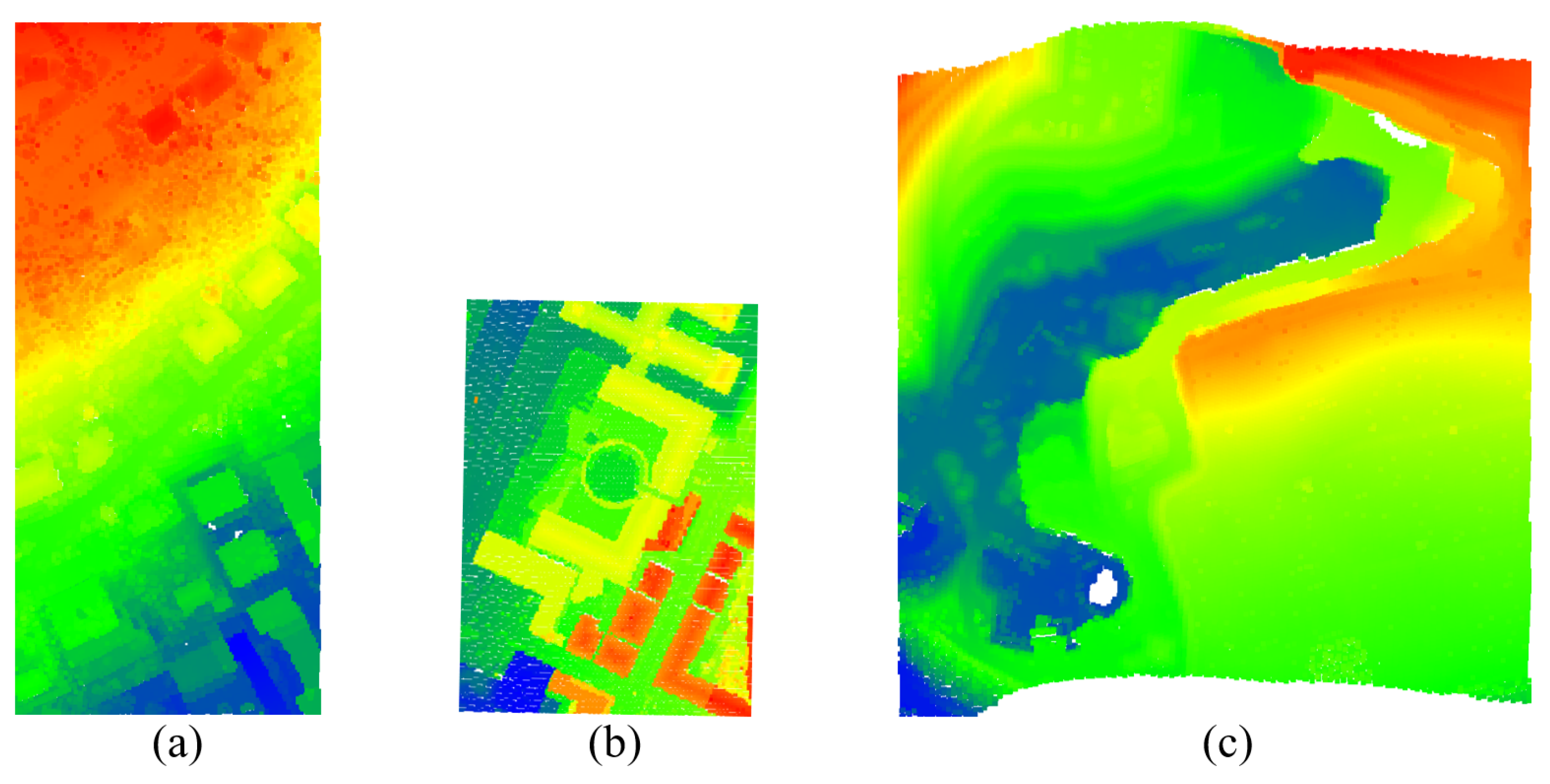
The benchmark dataset provided by International Society for Photogrammetry and Remote Sensing (ISPRS) was used to evaluate the performance of the proposed algorithm. The dataset was collected using the Optech Airborne Laser Terrain Mapping scanner in seven sites, including four urban sites (named Sites 1–4) and three rural sites (named Sites 5–7) [3]. As shown in Figure 4, non-ground objects with multiple types (e.g., buildings and vegetation) and variable sizes are contained in urban sites; the terrain (e.g., steep slopes and discontinuities) is the characteristic of rural sites. Details of each sample are listed in Table 1. The reference data was manually generated using prior knowledge and available airborne imagery.
The samples with rugged terrain and dense vegetation are limited in the ISPRS dataset. To comprehensively evaluate the performance of the proposed algorithm in different landscapes, we further tested the algorithm in four mountainous forested areas in the Open Topography dataset. All samples are presented in Figure 5. As shown in Table 2, the vegetation cover changes from 8.74% to 84.67%, and different terrain features (e.g., steep slopes, ridges, and valleys) are included in the samples. The reference data of the samples was generated by manual editing in CloudCompare software v2.11.3.

3.2. Parameter Setting

The structuring element size for initializing cloth is the only user-defined parameter. The threshold of the parameter should exceed the size of the largest object in a landscape to prevent the initialized cloth from being covered on non-ground objects. The parameter threshold in urban and rural samples was consistent with that in the literature [41], and that of the forested samples was set to 10 m.

3.3. Comparative Algorithms

In addition to CSF, eight reference algorithms published by ISRPS were used as comparative algorithms for urban and rural samples. For forested samples, the proposed algorithm was compared with the maximum slope filtering (MSF), progressive morphology filtering (PMF) and CSF algorithms, which are classical algorithms of slope-, morphology- and surface-based methods. MSF, PMF and CSF were implemented using the C++ programming language and the PCL library.

3.4. Accuracy Measures

Type I error (TI), type II error (TII) and total error (TE) were used to quantitatively assess the performance of the proposed algorithm. Type I error, type II error and total error are the proportions of ground points misclassified as non-ground points in reference ground points, non-ground points misclassified as ground points in reference non-ground points, and misclassified points in all points [28]. They are calculated by the following equations:
TI = a c
TII = b d
TE = a + b c + d
where a (b) is the number of ground (non-ground) points misclassified as non-ground (ground) points, and c (d) is the number of reference ground (non-ground) points.

4. Results and Discussion

4.1. Urban and Rural Samples

The type I, type II and total errors of ICSF are listed in Table 3. ICSF achieved an average total error of 4.03%. The total errors of ICSF did not exceed 5% in all samples except Samps 11, 23 and 53. The total errors are 9.74%, 7.4% and 6.23% in the three samples, respectively. In addition, the type II errors were large (>10%) in Samps 51, 52, 53 and 61. This is because the number of non-ground points is small, and misclassification of only a few non-ground points will produce a large type II error [26].
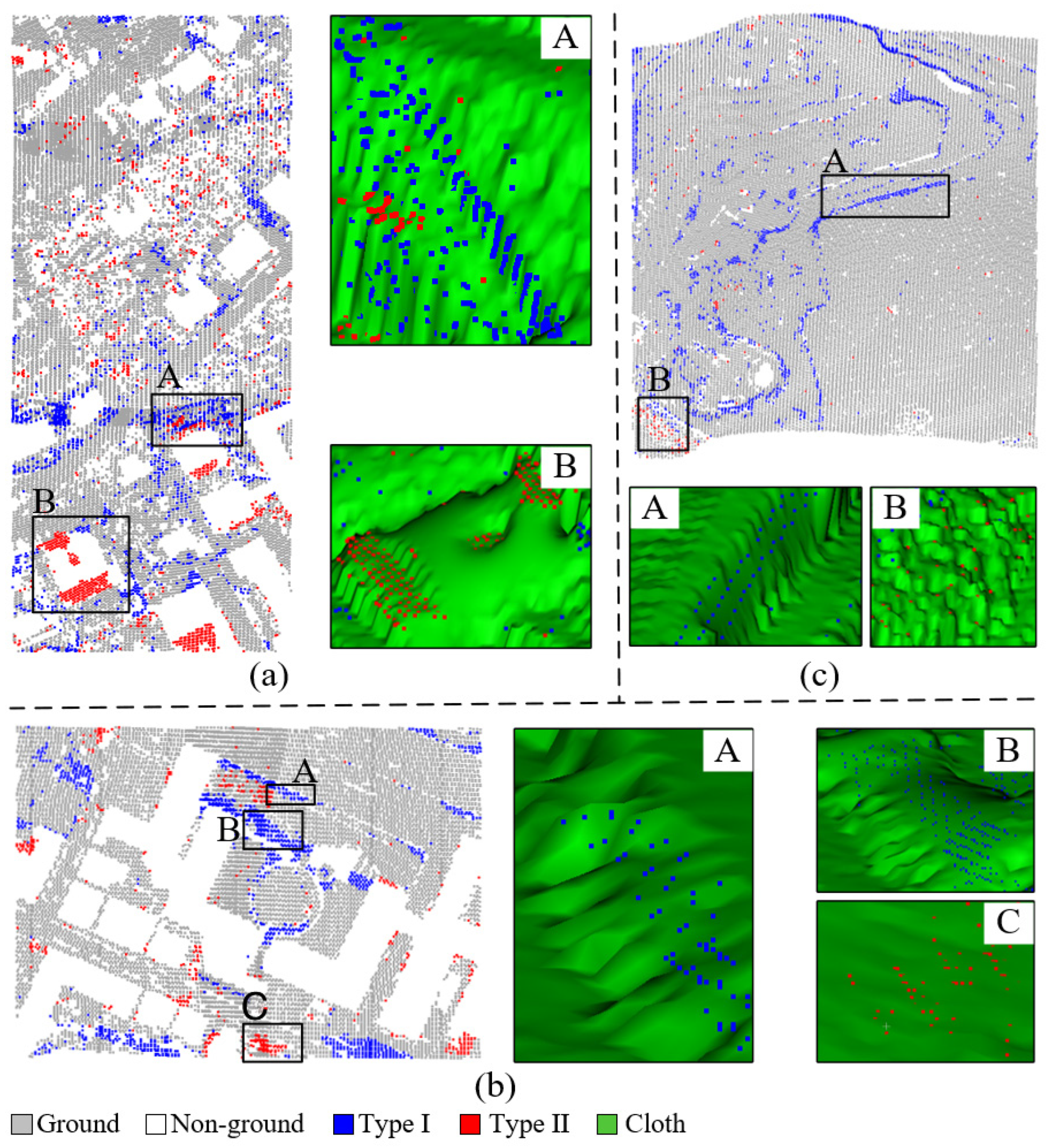
To illustrate the reason why ICSF had relatively poor results in Samps 11, 23 and 53, we visualized the distribution of their type I and II errors (Figure 6). In Samp11, the type I errors were mainly distributed on a fault scarp, as shown in the enlarged view A of Figure 6a. The slope of the fault scarp is close to 90°, which exhibits a similar character to building facades. Due to the extreme slope, the cloth cannot collide sufficiently with the fault scarp, resulting in the fault scarp not being covered by the cloth and thereby producing filtering errors. The type II errors were mainly distributed on the roof of a building, as shown in the enlarged view B of Figure 6a. The building is located on a hillside, and the height change between some parts of its roof and the hillside is not abrupt. This causes the cloth to stick to the roof, and in turn results in the roof points being misclassified as ground points [27]. In Samp23, the type I errors were distributed not only on a fault scarp, as shown in the enlarged view A of Figure 6b, but also on a raised terrain, as shown in the enlarged view B of Figure 6b. Unlike common raised terrain, the raised terrain has a large height change compared to the surrounding terrain, which exhibits a similar character to roofs of buildings. As a result, cloth cannot be collided with the raised terrain, generating inaccurate reference terrain. The ground points on the raised terrain are misclassified as non-ground points. The type II errors were mainly distributed on low non-ground objects, where the cloth was directly pasted after an external force operation. This causes the points on the low non-ground objects to be misclassified as ground points, due to inaccurate reference terrain [27]. In Samp53, the type I and II errors were mainly distributed on fault scarps and low non-ground objects, as shown in the enlarged views A and B of Figure 6c, due to the same reasons as in Samps 11 and 23.
The total errors of ICSF compared to CSF for all samples are shown in Table 4. ICSF obtained the lower type I errors in 14 of the 15 samples. In the remaining sample, the error difference between ICSF and CSF was slight, with a difference of 0.2%. This indicated that ICSF can more completely preserve the ground points than CSF. It benefits from the cloth initialization allowing the cloth to more completely cover various terrain features. ICSF generated the lower type II errors in 9 of the 15 samples, and the type II errors of the remaining samples were close to the results of CSF. Non-ground points can also be accurately removed by ICSF. This is because the terrain-adaptive thresholds ensure that the ground and non-ground points are more accurately distinguished, although cloth that more completely covers terrain increases the risk of type II errors [41]. On average, ICSF decreased the type I, type II and total errors by 39.17%, 25.91% and 39.12%, compared to CSF.
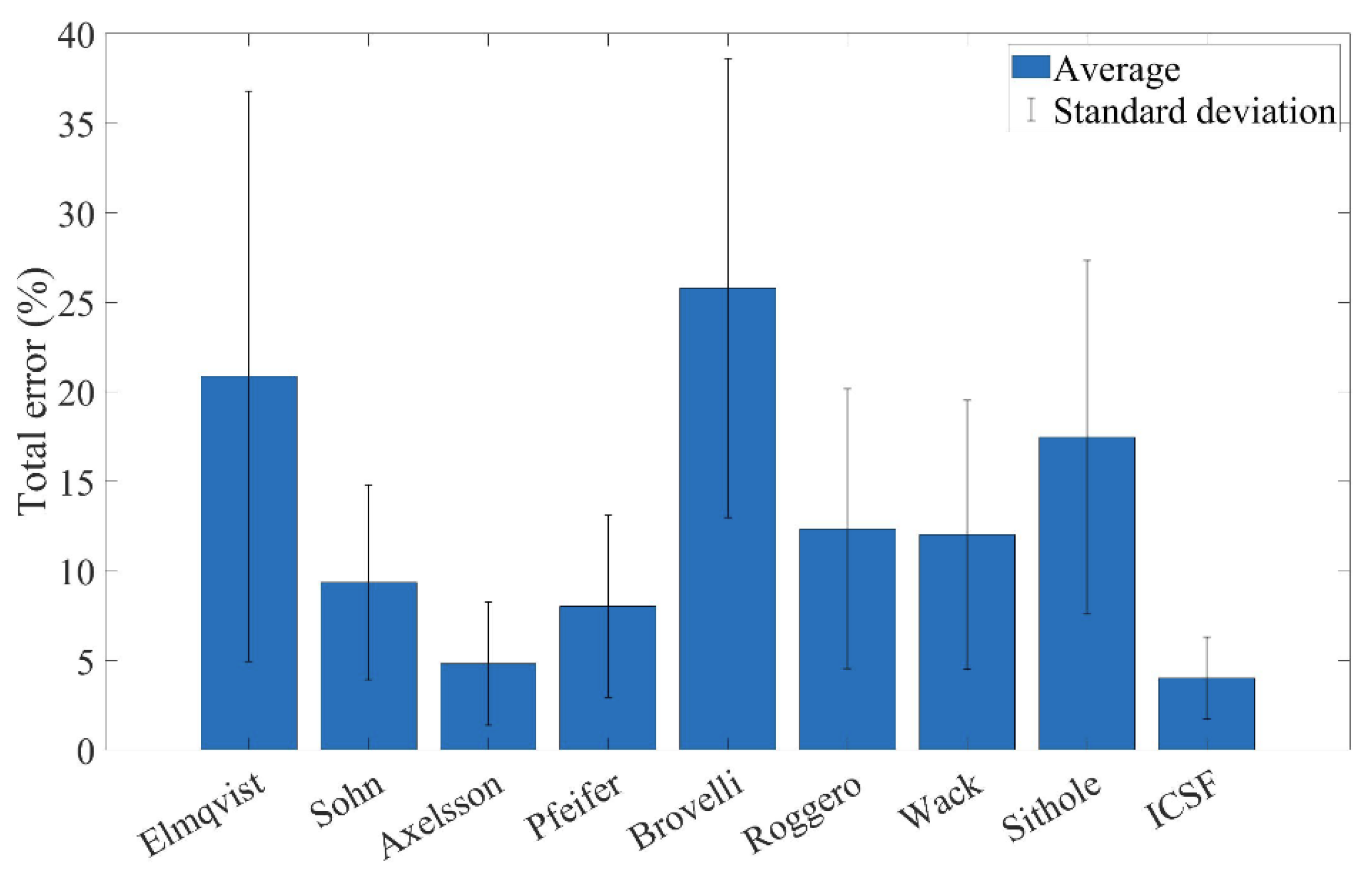
To further quantitatively evaluate the performance of ICSF, we compared the total errors with eight reference algorithms published by ISPRS. The principles of the eight algorithms are shown in Table 5, and detailed information of the algorithms can be found in [3]. As shown in Figure 7, ICSF achieved the lowest average value and standard deviation of total error, which demonstrated the superiority of ICSF in terms of accuracy and robustness. Additionally, the progressive TIN densification filtering (PTDF) algorithm proposed by Axelsson [42] performed better than other comparative methods. PTDF constructs a reference terrain using TIN, and then progressively adds ground points to update the reference terrain, based on the distances between points and the terrain. However, false ground points are not removed in PTDF, resulting in accumulated errors of reference terrain in subsequent iterations. Moreover, the local terrain with small areas cannot be accurately represented by TIN facets, since the vertical errors of LiDAR points may dominate the shape of TIN facets. The limitation of PTDF can be overcome by the internal force operation of ICSF.

4.2. Forested Samples

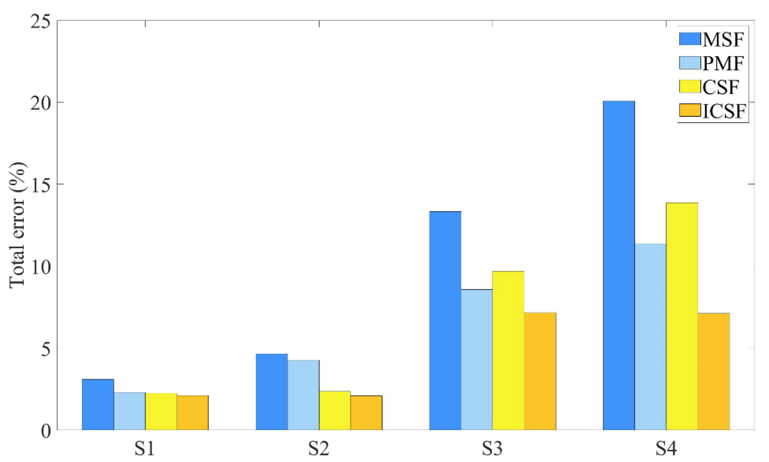
Table 6 exhibits the type I, type II and total errors of ICSF in all forested samples. We can see that ICSF produced lower total errors in S1 and S2 compared to S3 and S4. The first two samples consist of gentle slopes and dense vegetation, while the latter two samples have more complex terrain, including steep slopes and discontinuities. Overall, ICSF obtained an average total error of 4.62%.
Figure 8 shows the total errors of ICSF compared to classical filtering algorithms in the forested samples. All algorithms worked well in the samples with gentle slopes (i.e., S1 and S2), with a total error of less than 5%. ICSF obtained significantly lower total errors in the samples with steep slopes and discontinuities (i.e., S3 and S4). Overall, ICSF outperformed other filtering algorithms. More specifically, compared with MSF, PMF and CSF, ICSF reduced the average total error by 55.11%, 30.41% and 34.47%, respectively.
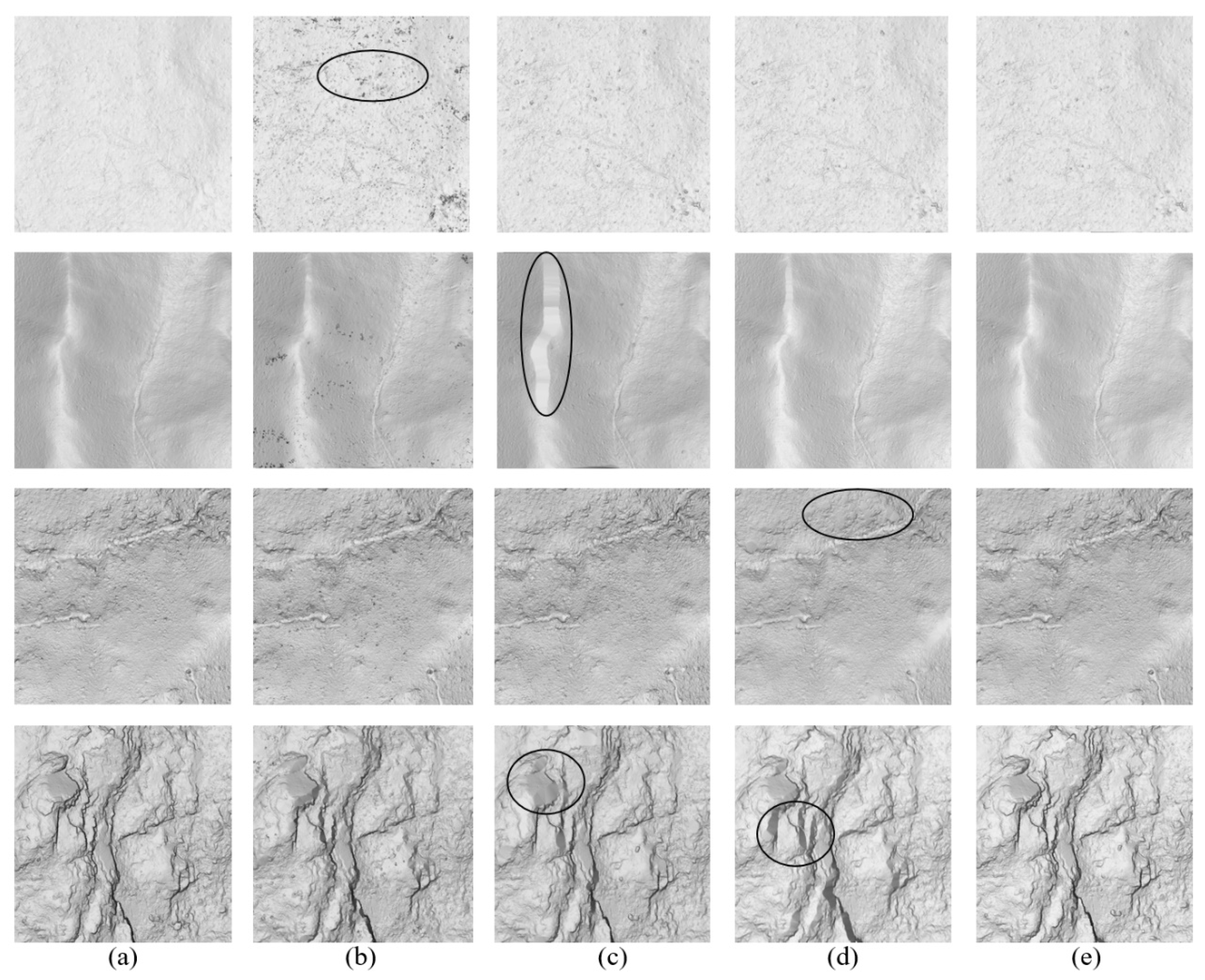
Figure 9 shows the digital terrain models (DTMs) of ICSF and classical filtering algorithms in all forested samples. PMF often misclassified vegetation points as ground points in S1 (see the ellipse in the first row of Figure 9b), because PMF considers an unclassified point as a ground point as long as there is a ground point with a threshold less than that of the unclassified point in a neighborhood [46]. On the contrary, ICSF identifies an unclassified point as a ground point when there are enough ground points around the unclassified point. Thus, ICSF can reduce the errors that occur when non-ground points are misjudged as ground points. PMF tended to misjudge ridge points as non-ground points in S2, due to erosion operations (see the ellipse in the second row of Figure 9c) [18,38]. However, ICSF can estimate the raised terrain by external force operations, thus preserving the ridge. In S3 and S4, PMF and CSF tended to smooth steep slopes (see the ellipses in the last two rows of Figure 9c,d), while ICSF can effectively estimate steep slopes through cloth initialization and external force operations, better preserving terrain details. Overall, ICSF performed better with respect to the preservation of steep slopes and discontinuities and vegetation removal.

5. Conclusions

This study aimed to improve the CSF algorithm for various areas including urban, rural and forested landscapes. Results showed that the ICSF algorithm outperformed the well-known filtering algorithms. The advantage of the ICSF algorithm lies within its ability to more completely preserve steep slopes and discontinuities, while accurately filtering out non-ground points. Moreover, ICSF can be used as a useful tool to filter airborne LiDAR data, due to its effectiveness, robustness and ease of use advantage. However, the proposed algorithm also has the limitation that the ground points on fault scarps and the building points on hillsides may be misclassified. This is essentially because these points violate the underlying assumption that the height change of terrain is gradual, while the height change between terrain and non-ground objects is abrupt. In the future, we will consider combining image data to reduce such errors.

Author Contributions

Conceptualization, S.C.; data curation, S.C.; formal analysis, S.C. and S.Y.; funding acquisition, S.C.; investigation, S.C.; methodology, S.C. and S.Y.; project administration, S.C., S.Y. and Z.H.; resources, S.C.; software, S.C.; supervision, S.Y.; validation, S.C. and S.Y.; visualization, S.C.; writing—original draft, S.C.; writing—review and editing, S.C., S.Y., Z.H. and Z.T. All authors have read and agreed to the published version of the manuscript.

Funding

This research was funded by the Open Fund of Key Laboratory of Mine Environmental Monitoring and Improving around Poyang Lake, Ministry of Natural Resources, grant number MEMI-2021-2022-03 and National Key R&D Program of China (2022YFB3903800).

Data Availability Statement

The authors do not have permission to share data.

Conflicts of Interest

The authors declare no conflict of interest.

References

  1. Wang, R.; Peethambaran, J.; Chen, D. LiDAR point clouds to 3-D urban models: A review. IEEE J. Sel. Top. Appl. Earth Obs. Remote Sens. 2018, 11, 606–627. [Google Scholar] [CrossRef]
  2. Yan, W.Y.; Shaker, A.; El-Ashmawy, N. Urban Land Cover Classification Using Airborne LiDAR Data: A Review. Remote Sens. Environ. 2015, 158, 295–310. [Google Scholar] [CrossRef]
  3. Sithole, G.; Vosselman, G. Experimental comparison of filter algorithms for bare-earth extraction from airborne laser scanning point clouds. ISPRS J. Photogramm. Remote Sens. 2004, 59, 85–101. [Google Scholar] [CrossRef]
  4. Meng, X.; Currit, N.; Zhao, K. Ground filtering algorithms for airborne LiDAR data: A review of critical issues. Remote Sens. 2010, 2, 833–860. [Google Scholar] [CrossRef] [Green Version]
  5. Chen, D.; Zhang, L.; Wang, Z.; Deng, H. A mathematical morphology-based multi-level filter of LiDAR data for generating DTMs. Sci. China Inf. Sci. 2012, 56, 1–14. [Google Scholar] [CrossRef] [Green Version]
  6. Guo, Q.; Li, W.; Yu, H.; Alvarez, O. Effects of topographic variability and LiDAR sampling density on several dem interpolation methods. Photogramm. Eng. Remote Sens. 2010, 76, 701–712. [Google Scholar] [CrossRef] [Green Version]
  7. Liu, X. Airborne LiDAR for DEM generation: Some critical issues. Prog. Phys. Geog. 2008, 32, 31–49. [Google Scholar]
  8. Wang, R. 3D building modeling using images and LiDAR: A review. Int. J. Image Data Fusion 2013, 4, 273–292. [Google Scholar] [CrossRef]
  9. Liu, K.; Ma, H.; Zhang, L.; Liang, X.; Chen, D.; Liu, Y. Roof segmentation from airborne LiDAR using octree-based hybrid region growing and boundary neighborhood verification voting. IEEE J. Sel. Top. Appl. Earth Obs. Remote Sens. 2023, 16, 2134–2146. [Google Scholar] [CrossRef]
  10. Shao, J.; Zhang, W.; Shen, A.; Mellado, N.; Cai, S.; Luo, L.; Wang, N.; Yan, G.; Zhou, G. Seed point set-based building roof extraction from airborne LiDAR point clouds using a top-down strategy. Autom. Constr. 2021, 126, 103660. [Google Scholar] [CrossRef]
  11. Sampath, A.; Shan, J. Segmentation and reconstruction of polyhedral building roofs from aerial LiDAR point clouds. IEEE Trans. Geosci. Remote Sens. 2010, 48, 1554–1567. [Google Scholar] [CrossRef]
  12. Rottensteiner, F.; Sohn, G.; Gerke, M.; Wegner, J.D.; Breitkopf, U.; Jung, J. Results of the ISPRS benchmark on urban object detection and 3D building reconstruction. ISPRS J. Photogramm. Remote Sens. 2014, 93, 256–271. [Google Scholar] [CrossRef]
  13. Cai, S.; Zhang, W.; Jin, S.; Shao, J.; Li, L.; Yu, S.; Yan, G. Improving the estimation of canopy cover from UAV-LiDAR data using a pit-free CHM-based method. Int. J. Digit. Earth 2021, 14, 1477–1492. [Google Scholar] [CrossRef]
  14. Brandtberg, T. Classifying individual tree species under leaf-off and leaf-on conditions using airborne lidar. ISPRS J. Photo-gramm. Remote Sens. 2007, 61, 325–340. [Google Scholar] [CrossRef]
  15. Hyyppä, J.; Yu, X.; Hyyppä, H.; Vastaranta, M.; Holopainen, M.; Kukko, A.; Kaartinen, H.; Jaakkola, A.; Vaaja, M.; Koskinen, J.; et al. Advances in forest inventory using airborne laser scanning. Remote Sens. 2012, 4, 1190–1207. [Google Scholar] [CrossRef] [Green Version]
  16. Dai, W.; Guan, Q.; Cai, S.; Liu, R.; Chen, R.; Liu, Q.; Chen, C.; Dong, Z. A comparison of the performances of un-manned-aerial-vehicle (UAV) and terrestrial laser scanning for forest plot canopy cover estimation in pinus massoniana forests. Remote Sens. 2022, 14, 1188. [Google Scholar] [CrossRef]
  17. Popescu, S.C. Estimating biomass of individual pine trees using airborne lidar. Biomass Bioenergy 2007, 31, 646–655. [Google Scholar] [CrossRef]
  18. Cai, S.; Yu, S. Filtering airborne LiDAR data in forested environments based on multi-directional narrow window and cloth simulation. Remote Sens. 2023, 15, 1400. [Google Scholar] [CrossRef]
  19. Bigdeli, B.; Amirkolaee, H.A.; Pahlavani, P. DTM extraction under forest canopy using LiDAR data and a modified invasive weed optimization algorithm. Remote Sens. Environ. 2018, 216, 289–300. [Google Scholar] [CrossRef]
  20. Véga, C.; Durrieu, S.; Morel, J.; Allouis, T. A sequential iterative dual-filter for Lidar terrain modeling optimized for complex forested environments. Comput. Geosci. 2012, 44, 31–41. [Google Scholar] [CrossRef]
  21. Kobler, A.; Pfeifer, N.; Ogrinc, P.; Todorovski, L.; Oštir, K.; Džeroski, S. Repetitive interpolation: A robust algorithm for DTM generation from aerial laser scanner data in forested terrain. Remote Sens. Environ. 2007, 108, 9–23. [Google Scholar] [CrossRef]
  22. Montealegre, A.L.; Lamelas, M.T.; De La Riva, J. A comparison of open-source LiDAR filtering algorithms in a mediterranean forest environment. IEEE J. Sel. Top. Appl. Earth Obs. Remote Sens. 2015, 8, 4072–4085. [Google Scholar] [CrossRef] [Green Version]
  23. Chen, Q.; Wang, H.; Zhang, H.; Sun, M.; Liu, X. A point cloud filtering approach to generating DTMs for steep mountainous areas and adjacent residential areas. Remote Sens. 2016, 8, 71. [Google Scholar] [CrossRef] [Green Version]
  24. Zhao, X.; Guo, Q.; Su, Y.; Xue, B. Improved progressive TIN densification filtering algorithm for airborne LiDAR data in forested areas. ISPRS J. Photogramm. Remote Sens. 2016, 117, 79–91. [Google Scholar] [CrossRef] [Green Version]
  25. Chen, C.; Guo, J.; Wu, H.; Li, Y.; Shi, B. Performance comparison of filtering algorithms for high-density airborne lidar point clouds over complex landscapes. Remote Sens. 2021, 13, 2663. [Google Scholar] [CrossRef]
  26. Chen, C.; Wang, M.; Chang, B.; Li, Y. Multi-level interpolation-based filter for airborne LiDAR point clouds in forested areas. IEEE Access 2020, 8, 41000–41012. [Google Scholar] [CrossRef]
  27. Zhang, W.; Qi, J.; Wan, P.; Wang, H.; Xie, D.; Wang, X.; Yan, G. An easy-to-use airborne lidar data filtering method based on cloth simulation. Remote Sens. 2016, 8, 501. [Google Scholar] [CrossRef]
  28. Vosselman, G. Slope based filtering of laser altimetry data. Int. Arch. Photogramm. Remote Sens. 2000, 33, 935–942. [Google Scholar]
  29. Meng, X.; Wang, L.; Silván-Cárdenas, J.L.; Currit, N. A multi-directional ground filtering algorithm for airborne LIDAR. ISPRS J. Photogramm. Remote Sens. 2009, 64, 117–124. [Google Scholar] [CrossRef] [Green Version]
  30. Shan, J.; Aparajithan, S. Urban DEM generation from raw lidar data. Photogramm. Eng. Remote Sens. 2005, 71, 217–226. [Google Scholar] [CrossRef] [Green Version]
  31. Chen, Z.; Gao, B.; Devereux, B. State-of-the-Art: DTM generation using airborne LIDAR data. Sensors 2017, 17, 150. [Google Scholar] [CrossRef] [Green Version]
  32. Susaki, J. Adaptive slope filtering of airborne lidar data in urban areas for digital terrain model (DTM) generation. Remote Sens. 2012, 4, 1804–1819. [Google Scholar] [CrossRef] [Green Version]
  33. Zhang, K.; Chen, S.-C.; Whitman, D.; Shyu, M.-L.; Yan, J.; Zhang, C. A progressive morphological filter for removing nonground measurements from airborne LIDAR data. IEEE Trans. Geosci. Remote Sens. 2003, 41, 872–882. [Google Scholar] [CrossRef] [Green Version]
  34. Yang, B.; Huang, R.; Dong, Z.; Zang, Y.; Li, J. Two-step adaptive extraction method for ground points and breaklines from lidar point clouds. ISPRS J. Photogramm. Remote Sens. 2016, 119, 373–389. [Google Scholar] [CrossRef]
  35. Chen, Q.; Gong, P.; Baldocchi, D.; Xie, G. Filtering airborne laser scanning data with morphological methods. Photogramm. Eng. Remote Sens. 2007, 73, 175–185. [Google Scholar] [CrossRef] [Green Version]
  36. Tan, Y.; Wang, S.; Xu, B.; Zhang, J. An improved progressive morphological filter for UAV-based photogrammetric point clouds in river bank monitoring. ISPRS J. Photogramm. Remote Sens. 2018, 146, 421–429. [Google Scholar] [CrossRef]
  37. Li, Y.; Yong, B.; Wu, H.; An, R.; Xu, H. An Improved top-hat filter with sloped brim for extracting ground points from airborne LiDAR point clouds. Remote Sens. 2014, 6, 12885–12908. [Google Scholar] [CrossRef] [Green Version]
  38. Hui, Z.; Hu, Y.; Yevenyo, Y.Z.; Yu, X. An improved morphological algorithm for filtering airborne LiDAR point cloud based on multi-level kriging interpolation. Remote Sens. 2016, 8, 35. [Google Scholar] [CrossRef] [Green Version]
  39. Mongus, D.; Lukač, N.; Žalik, B. Ground and building extraction from LiDAR data based on differential morphological profiles and locally fitted surfaces. ISPRS J. Photogramm. Remote Sens. 2014, 93, 145–156. [Google Scholar] [CrossRef]
  40. Pingel, T.J.; Clarke, K.C.; McBride, W.A. An improved simple morphological filter for the terrain classification of airborne LIDAR data. ISPRS J. Photogramm. Remote Sens. 2013, 77, 21–30. [Google Scholar] [CrossRef]
  41. Zhang, J.; Lin, X. Filtering airborne LiDAR data by embedding smoothness-constrained segmentation in progressive TIN densification. ISPRS J. Photogramm. Remote Sens. 2013, 81, 44–59. [Google Scholar] [CrossRef]
  42. Axelsson, P. DEM generation from laser scanner data using adaptive tin models. Int. Arch. Photogramm. Remote Sens. 2020, 33, 111–118. [Google Scholar]
  43. Nie, S.; Wang, C.; Dong, P.; Xi, X.; Luo, S.; Qin, H. A revised progressive TIN densification for filtering airborne LiDAR data. Measurement 2017, 104, 70–77. [Google Scholar] [CrossRef]
  44. Hu, H.; Ding, Y.; Zhu, Q.; Wu, B.; Lin, H.; Du, Z.; Zhang, Y.; Zhang, Y. An adaptive surface filter for airborne laser scanning point clouds by means of regularization and bending energy. ISPRS J. Photogramm. Remote Sens. 2014, 92, 98–111. [Google Scholar] [CrossRef]
  45. Evans, J.S.; Hudak, A.T. A multiscale curvature algorithm for classifying discrete return LiDAR in forested environments. IEEE Trans. Geosci. Remote Sens. 2007, 45, 1029–1038. [Google Scholar] [CrossRef]
  46. Chen, C.; Li, Y.; Li, W.; Dai, H. A multiresolution hierarchical classification algorithm for filtering airborne LiDAR data. ISPRS J. Photogramm. Remote Sens. 2013, 82, 1–9. [Google Scholar] [CrossRef]
  47. Meng, X.; Lin, Y.; Yan, L.; Gao, X.; Yao, Y.; Wang, C.; Luo, S. Airborne LiDAR point cloud filtering by a multilevel adaptive filter based on morphological reconstruction and thin plate spline interpolation. Electronics 2019, 8, 1153. [Google Scholar] [CrossRef] [Green Version]
  48. Wei, L.; Yang, B.; Jiang, J.; Cao, G.; Wu, M. Vegetation filtering algorithm for UAV-borne lidar point clouds: A case study in the middle-lower Yangtze River riparian zone. Int. J. Remote Sens. 2016, 38, 2991–3002. [Google Scholar] [CrossRef]
  49. Zhao, X.; Su, Y.; Li, W.; Hu, T.; Liu, J.; Guo, Q. A comparison of LiDAR filtering algorithms in vegetated mountain areas. Can. J. Remote Sens. 2018, 44, 287–298. [Google Scholar] [CrossRef]
  50. Yang, A.; Wu, Z.; Yang, F.; Su, D.; Ma, Y.; Zhao, D.; Qi, C. Filtering of airborne LiDAR bathymetry based on bidirectional cloth simulation. ISPRS J. Photogramm. Remote Sens. 2020, 163, 49–61. [Google Scholar] [CrossRef]
  51. Wan, P.; Zhang, W.; Skidmore, A.K.; Qi, J.; Jin, X.; Yan, G.; Wang, T. A simple terrain relief index for tuning slope-related parameters of LiDAR ground filtering algorithms. ISPRS J. Photogramm. Remote Sens. 2018, 143, 181–190. [Google Scholar] [CrossRef]
  52. Hui, Z.; Wang, L.; Ziggah, Y.Y.; Cai, S.; Xia, Y. Automatic morphological filtering algorithm for airborne lidar data in urban areas. Appl. Opt. 2019, 58, 1164–1173. [Google Scholar] [CrossRef] [PubMed]
  53. Hui, Z.; Jin, S.; Xia, Y.; Nie, Y.; Xie, X.; Li, N. A mean shift segmentation morphological filter for airborne LiDAR DTM extraction under forest canopy. Opt. Laser Technol. 2021, 136, 106728. [Google Scholar] [CrossRef]
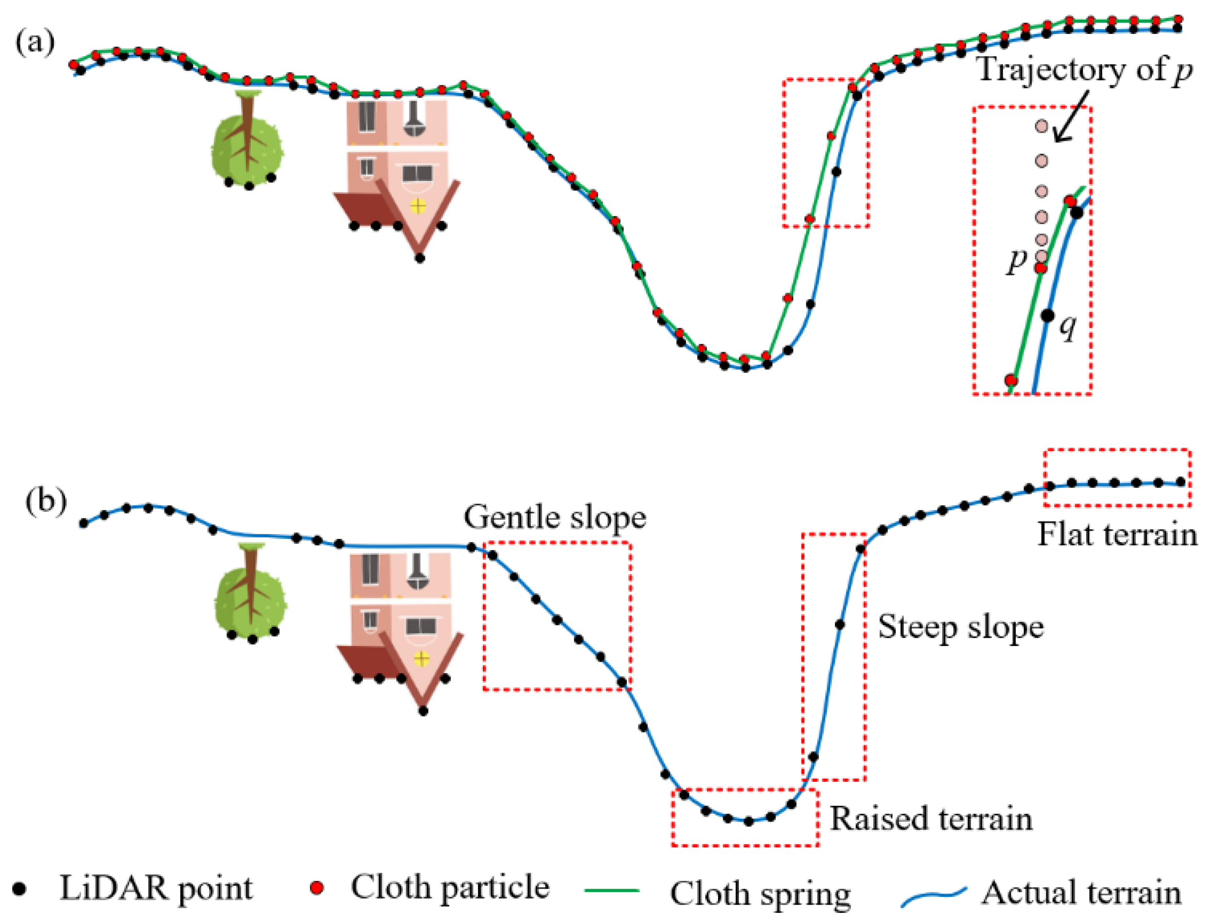
Figure 1. Limitations of CSF: (a) steep slopes cannot be covered by cloth; (b) a single cloth rigidness is not suitable for the scene containing multiple terrain features, including flat terrain, gentle slopes, steep slopes and raised terrain.
Forests 14 01520 g001
Figure 2. Flowchart of ICSF. The upper and lower parts are the main steps of the proposed algorithm and the results for each step for sample data.
Forests 14 01520 g002
Figure 3. Main steps in cloth initialization: (a) cloth modeling. The cloth is modeled as a grid consisting of particles and springs. The cloth values are the elevations of the highest points in the grid cells, and the springs are constructed based on particles and their eight neighboring particles; (b) dilation operation. The particle values are adjusted to the local maximum values; (c) erosion operation. The particle values are adjusted to the local minimum values.
Forests 14 01520 g003
Figure 4. Representative urban and rural samples: (a) Samp11; (b) Samp23; (c) Samp53. A large amount of vegetation and many buildings are distributed on the hillside for S11. Large, irregularly shaped buildings are characteristic of S23. In S53, there are many discontinuities and steep slopes on the ground surface.
Forests 14 01520 g004
Figure 5. Forested samples: (a) S1; (b) S2; (c) S3; (d) S4. The four samples are characterized by gentle slopes and dense vegetation, undulating terrain and dense vegetation, steep slopes and dense vegetation, and steep slopes and discontinuities, respectively.
Forests 14 01520 g005
Figure 6. Error distributions of ICSF in (a) Samp11, (b) Samp23 and (c) Samp53. A, B, and C represent the numbers of the enlarged figures. In the three samples, the two types of errors are mainly distributed on fault scarps and raised terrain, and low non-ground objects and building roofs, respectively.
Forests 14 01520 g006
Figure 7. Total errors compared to other published algorithms. ICSF obtained the lowest average value and standard deviation of total error for all 15 samples.
Forests 14 01520 g007
Figure 8. Total errors compared to other published algorithms in forested samples. ICSF showed greater advantage in terms of accuracy, especially in complex terrain.
Forests 14 01520 g008
Figure 9. Comparison of MSF, PMF, CSF and ICSF in terms of the preservation of steep slopes and discontinuities, and vegetation removal. DTMs generated using (a) reference data, (b) MSF, (c) PMF, (d) CSF and (e) ICSF in all forested samples. Overall, ICSF performed better in terms of the preservation of steep slopes and discontinuities and vegetation removal.
Forests 14 01520 g009
Table 1. Features and statistics of all samples in urban and rural sites.
SiteSampleFeatureReference (Points)
GroundNon-Ground
111Mixture of vegetation and buildings on hillside21,78616,224
12Mixture of vegetation and buildings26,69125,428
221Road with bridge10,0852875
22Irregular buildings and bridge22,50410,202
23Large, irregularly shaped buildings13,22311,872
24Steep slopes54342058
331Complex buildings15,55613,306
441Irregular buildings56025629
42Railway station with trains12,44330,027
551Vegetation on slopes13,9503895
52Low vegetation on slopes20,1122362
53Discontinuities and steep slopes32,9891389
54Low buildings39834625
661Discontinuities33,8541206
771Underpass and bridge13,8751770
Table 2. Features and statistics of all samples in forested sites.
SampleFeatureVegetation Cover (%)Reference (Points)
GroundNon-Ground
S1Gentle slopes and dense vegetation80.08473,5381,493,507
S2Undulating terrain and dense vegetation84.67261,242518,792
S3Steep slopes and dense vegetation 74.45514,925819,264
S4Steep slopes and discontinuities8.74298,95544,499
Table 3. Type I, type II and total errors of ICSF in urban and rural samples (%).
EnvironmentSampleTITIITE
UrbanSamp1111.557.319.74
Samp121.974.042.98
Samp210.725.981.89
Samp224.964.764.9
Samp239.984.547.4
Samp242.917.584.19
Samp310.296.343.08
Samp413.281.432.37
Samp420.973.93.04
RuralSamp510.3112.482.96
Samp523.8513.634.88
Samp535.9911.886.23
Samp540.77.494.35
Samp610.4612.270.86
Samp710.589.661.61
Average3.237.554.03
Note: I, II and TE denote the type I error, type II error and total error, respectively.
Table 4. Accuracy comparison between CSF and ICSF (%).
SampleCSFICSF
TITIITETITIITE
Samp1119.26.6613.8511.557.319.74
Samp122.994.293.631.974.042.98
Samp210.525.811.690.725.981.89
Samp227.3215.239.794.964.764.9
Samp2312.1812.712.439.984.547.4
Samp248.856.958.332.917.584.19
Samp310.4815.657.470.296.343.08
Samp413.712.212.973.281.432.37
Samp422.039.297.160.973.93.04
Samp511.1710.173.130.3112.482.96
Samp525.22216.873.8513.634.88
Samp5312.499.4312.375.9911.886.23
Samp540.988.444.990.77.494.35
Samp611.385.561.520.4612.270.86
Samp711.119.443.170.589.661.61
Average5.3110.196.623.237.554.03
Note: I, II and TE denote the type I error, type II error and total error, respectively.
Table 5. Description of comparative algorithms [3].
ParticipantFilter Description
ElmqvistActive contours
SohnRegularization method
AxelssonProgressive TIN densification
PfeiferHierarchical robust interpolation
BrovelliSpline interpolation
RoggeroModified slope-based filter
WackHierarchical modified block minimum
SitholeModified slope-based filter
Table 6. Type I, type II and total errors of ICSF in forested samples (%).
EnvironmentSampleTITIITE
ForestS10.122.752.12
S20.412.942.09
S35.148.447.17
S47.35.957.12
Average3.245.024.62
Note: I, II and TE denote the type I error, type II error and total error, respectively.
Disclaimer/Publisher’s Note: The statements, opinions and data contained in all publications are solely those of the individual author(s) and contributor(s) and not of MDPI and/or the editor(s). MDPI and/or the editor(s) disclaim responsibility for any injury to people or property resulting from any ideas, methods, instructions or products referred to in the content.