Estimation of Forest Height Using Google Earth Engine Machine Learning Combined with Single-Baseline TerraSAR-X/TanDEM-X and LiDAR

Abstract

Forest height plays a crucial role in various fields, such as forest ecology, resource management, natural disaster management, and environmental protection. In order to obtain accurate and efficient measurements of forest height over large areas, in this study, Terra Synthetic Aperture Radar-X and the TerraSAR-X Add-on for Digital Elevation Measurement (TerraSAR-X/TanDEM-X), Sentinel-2A, and Shuttle Radar Topography Mission (SRTM) data were used, and various feature combinations were established in conjunction with measurements from Light Detection and Ranging (LiDAR). Classification and regression tree (CART), gradient-boosting decision tree (GBDT), random forest (RF), and support vector machine (SVM) algorithms were employed to estimate forest height in the study area. Independent validation on the basis of LiDAR forest height samples showed the following results: (1) Regarding feature combinations, the combination of coherence and decorrelation of volume scattering provided by TerraSAR-X/TanDEM-X data outperformed the combination of backscatter coefficient and local incidence angle, as well as the combination of coherence, decorrelation of volume scattering, backscatter coefficient, and local incidence angle. The best results (R² = 0.67, RMSE = 2.89 m) were achieved with the combination of coherence and decorrelation of volume scattering using the GBDT and RF algorithms. (2) In terms of machine learning methods, the GBDT algorithm proved suitable for estimating forest height. The most effective approach for forest height mapping involved combining the GBDT algorithm with coherence, decorrelation of volume scattering, and a small amount of LiDAR forest height data, used as training data.

1. Introduction

Forestry personnel require accurate and detailed height data to monitor the health and damage status of forests, optimize afforestation processes, and estimate the general height, quantity, and value of forest stands [1]. Additionally, forest height is a crucial factor in estimating forest carbon stock and biomass. Obtaining accurate and efficient forest height information over large areas is of significant importance for forest inventory and precision management, and in carbon trading markets [2,3,4,5]. The traditional method of forest height assessment based on the sampling of standard samples is not only time consuming and labor intensive, but is also incapable of providing continuous forest height data, thus no longer meeting the requirements of modern forest resource management and ecological environmental scientific research [6]. Remote sensing technology offers an efficient alternative for estimating the structural parameters of forests at regional and global scales. Currently, the remote sensing technologies employed for regional forest height mapping primarily include Light Detection and Ranging (LiDAR), photogrammetry, and Synthetic Aperture Radar (SAR). However, the exorbitant cost of LiDAR data, coupled with the utilization of LiDAR and photogrammetry is constrained by adverse weather conditions such as clouds and fog, limiting their potential in large-scale and continuous forest height mapping [7,8]. Synthetic Aperture Radar (SAR) technology, known for its excellent penetration capability, overcomes the limitations of optical remote sensing by effectively acquiring forest information under cloudy, overcast, and nighttime conditions [9,10,11].

Currently, there are two main approaches to estimating forest height using single-baseline, single-polarization TerraSAR-X/TanDEM-X data: (1) subtracting a known high-precision Digital Elevation Model (DEM) from the Digital Surface Model (DSM) obtained from Interferometric Synthetic Aperture Radar (InSAR) to derive the height of the forest’s effective scattering centers. This height has a good correlation with the actual forest height. However, the specific position of the scattering centers is influenced by forest structure and microwave frequency, requiring calibration with field measurements for accurate estimation of forest height. This method is limited in its applicability for large-scale estimation of forest height due to its dependence on high-precision DEM [12,13]. (2) X-band Polarimetric Interferometric Synthetic Aperture Radar (PolInSAR) estimation of forest height assumes zero surface scattering contributions and average extinction coefficient within the forest, deriving forest height directly from coherence coefficients [14,15,16]. This method overlooks the contribution of surface scattering in sparsely vegetated or low-vegetation areas, and the X-band SAR signal is significantly attenuated when penetrating the vegetation layer, making the assumption of zero extinction coefficient unrealistic [17,18,19].

Machine learning algorithms, with their precise classification and regression capabilities, fewer parameter settings, and high ability to integrate multisource data, have found extensive application in a diversity of fields, including forest health [20], forest fires [21], forest change [22], and forest biomass [23]. Using forest height inversion, in 2012, Chen et al. [24] estimated forest height in a research area in Quebec, Canada, by combining LiDAR data, Quickbird imagery, and SVM Regression. In 2018, Gu et al. [25] estimated forest height in the western Greater Khingan Mountains, China, by combining geometric optical model of sloping terrain, Landsat 7 ETM+, and airborne LiDAR data using neural networks and look-up table methods. In 2018, García et al. [26] estimated forest height on the basis of LiDAR data, multispectral data, and SAR backscattering information combined with SVM. In 2020, Li et al. [27] estimated forest height using Sentinel-1, Sentinel-2, ICESat-2, and Landsat-8 data, combined with the random forest and deep learning algorithms. In 2019, Brigot et al. [28] explored the potential of combining random forest and neural networks to merge PolInSAR data with LiDAR height. In 2019, Xie et al. [29] proposed a method for merging LiDAR and multibaseline PolInSAR data to improve the estimation of forest height. In 2018, Pourshamsi et al. [30] integrated PolInSAR components and LiDAR-derived height using SVM to improve forest height estimation. In 2018, Pourshamsi et al. [31] studied the combination of polarimetric SAR parameters extracted from different decomposition techniques (H/A/Alpha) and LiDAR data, using SVM to estimate forest height, achieving good results. However, in this approach, LiDAR data must be collected from the entire SAR image range for feature combination training, and LiDAR data covering the entire SAR image are not often available, and the study only evaluated the performance of SVM. In 2021, Pourshamsi et al. [32] estimated tropical forest height based on Polarimetric Synthetic Aperture Radar (PolSAR) data and airborne LiDAR using subsets of the LiDAR data to establish the relationship between multisource data features and forest height, estimating forest height within the SAR image range [32].

Most studies evaluated the performance of optical remote sensing imagery, satellite/airborne PolInSAR data, and PolSAR data in estimating forest height. However, further evaluation regarding the performance of SAR interferometric information, scattering information, and LiDAR data combined with different machine learning algorithms for large-scale estimation of forest height is necessary. The TerraSAR-X/TanDEM-X launched by the German Aerospace Center operates in a bistatic interferometric mode, unaffected by temporal decorrelation, and provides high-quality InSAR data [33,34].

This study focuses on the research area covered by airborne LiDAR data in Guigang City, Guangxi Zhuang Autonomous Region. The main data sources used are coherence, decorrelation of volume scattering, backscatter coefficient and local incidence angle obtained from TerraSAR-X/TanDEM-X, with the selection of spectral and terrain data related to forest height as auxiliary, in combination with LiDAR forest height as samples. The performance of different machine learning algorithms in estimating forest height is compared, and the potential of interferometric, backscatter coefficient, and local incidence angle information in forest height estimation is evaluated. Finally, a high-precision spatial distribution map of forest height is generated, providing a basis for efficient forest height inversion.

2. Materials and Methods

2.1. Study Area

The study area is situated in the northwestern part of Guigang City, Guangxi Zhuang Autonomous Region, southern China (109°11′~110°39′ E, 22°39′~24°2′ N), in the midstream of the Xijiang River, which is the main stem of the Pearl River Basin. It falls within the subtropical monsoon climate zone. The terrain consists of mountainous and hilly basins, with an average elevation of 52 m. The topography is relatively gentle, with most slopes below 10 degrees. The fraction of vegetation cover is approximately 68%, dominated by eucalyptus, pine, and fir trees, among others. Figure 1 presents the study area and the different tree species within sample plots. The yellow rectangular box represents the study area boundary (coverage of airborne LiDAR data), while the red rectangular box represents the SAR data coverage (main image).

2.2. Data Acquisition and Processing

2.2.1. TerraSAR-X/TanDEM-X Data

The TerraSAR-X/TanDEM-X mission involves the close-formation flying of two X-band SAR satellites to acquire single-pass interferometric SAR data. The data are collected in a bistatic mode, where one satellite acts as both the transmitter and receiver, while the other satellite functions solely as a receiver of electromagnetic waves. This study uses descending-orbit SAR data in TerraSAR-X/TanDEM-X strip mode, acquired on 7 October 2020. The interferometric pair consists of registered master and slave complex images, which are used to calculate coherence, decorrelation of volume scattering, backscatter coefficient, and local incidence angle. The data are geocoded and resampled to a spatial resolution of 12 m. The fundamental details of the interferometric pair are displayed in

Table 1. Basic information of TerraSAR-X/TanDEM-X Data.

Acquisition Time	Height of Ambiguity (m)	Effective Baseline (m)	Incidence Angle (°)	Polarization Mode	kz (rad/m)	Resolution (Rg × Az) (m)
2020-10-07	32.7	203.4	40.6	HH	0.19	2.71 × 3.30

.

2.2.2. Sentinel-2A Data

Sentinel-2A is composed of two satellites and equipped with a Multi-Spectral Instrument (MSI), which provides spatial resolutions of 10 m, 20 m, and 60 m. Each satellite has a revisit period of 10 days. The Sentinel-2A data utilized in the study have a spatial resolution of 10 m. On the GEE platform, the corresponding image collection for Sentinel-2A is “COPERNICUS/S2_SR”. To calculate the fraction of vegetation cover (FVC), Sentinel-2A image data with cloud cover below 5% are selected within the SAR image range. Subsequently, the FVC is resampled to a spatial resolution of 12 m.

2.2.3. SRTM Data

Shuttle Radar Topography Mission (SRTM) is a DEM dataset obtained by NASA and NIMA during a space shuttle radar terrain mapping mission in the year 2000. It covers a significant portion of land areas at latitudes between 60° N and 54° S. In this study, on the GEE platform, the elevation band of the USGS/SRTMGL1_003 dataset is selected. The spatial resolution of the data was initially 30 m. Subsequently, these data were resampled to a 12 m resolution, followed by the computation of slope and aspect.

2.2.4. ESA WorldCover 10 m 2020 Data

The European Space Agency (ESA) provides the WorldCover 10 m 2020 product, which is a global land cover map for the year 2020, featuring a spatial resolution of 10 m. This product is based on data from the Sentinel-2 and Sentinel-1 satellites. The WorldCover product consists of 11 land cover categories and is part of the 5th Earth Observation Envelope Programme (EOEP-5). In this study, on the GEE cloud platform, the ESA/WorldCover/v100 dataset is selected. It is cropped according to the extent of the SAR image, downloaded locally, and resampled to a 12 m spatial resolution to obtain the forest areas.

2.2.5. Airborne LiDAR Data

(1)

Data Acquisition

The airborne LiDAR data was acquired in September 2019 using a P750 aircraft equipped with the RIEGL-VQ-1560i airborne laser scanning system. The aircraft flew at an altitude of 2500 m above the ground. The adjacent flight lines had an approximate overlap of 20%, and the minimum LiDAR point cloud density was set to be greater than or equal to 3 points per square meter. The point cloud data was processed using the RiPROCESS 1.9.1 software and a LiDAR point cloud processing system. The processing involved noise removal and classification of ground and non-ground points. This resulted in the generation of DSM and DEM with a spatial resolution of 2 m. These models were then resampled to a 12 m resolution. The LiDAR forest height was obtained by subtracting the LiDAR DEM from the LiDAR DSM, representing the true height of the forest, and used as reference height data.

(2)

Sample Point Collection

A random sampling method was employed within the ESA WorldCover forest area, with a coherence threshold of ≥0.3. The sampling spacing was set to be ≥12 m. Within the LiDAR forest height range, three different height categories were defined: (0–10 m, 10–20 m, 20–30 m). A total of 6225 sample points were selected, proportionally distributed among the height categories based on their respective proportions. These sample points accounted for approximately 15% of the entire LiDAR dataset (41,000 pixels), as shown in

Table 2. Information of sample points.

Data	Count	Maximum Value (m)	Minimum Value (m)	Average Value (m)	Standard Deviation (m)	Number of Samples in the Range of 0–10 m	Number of Samples in the Range of 10–20 m	Number of Samples in the Range of 20–30 m
LiDAR forest height sample points	6225	24.7	0.1	8.2	5.0	4193	2007	25

and Figure 2.

2.3. Methods

This study investigates the research technology roadmap, shown in Figure 3, by employing various algorithms, including CART, GBDT, RF, and SVM to estimate forest height. A comparison is made with the DSM-DEM differencing method and the SINC function modeling method.

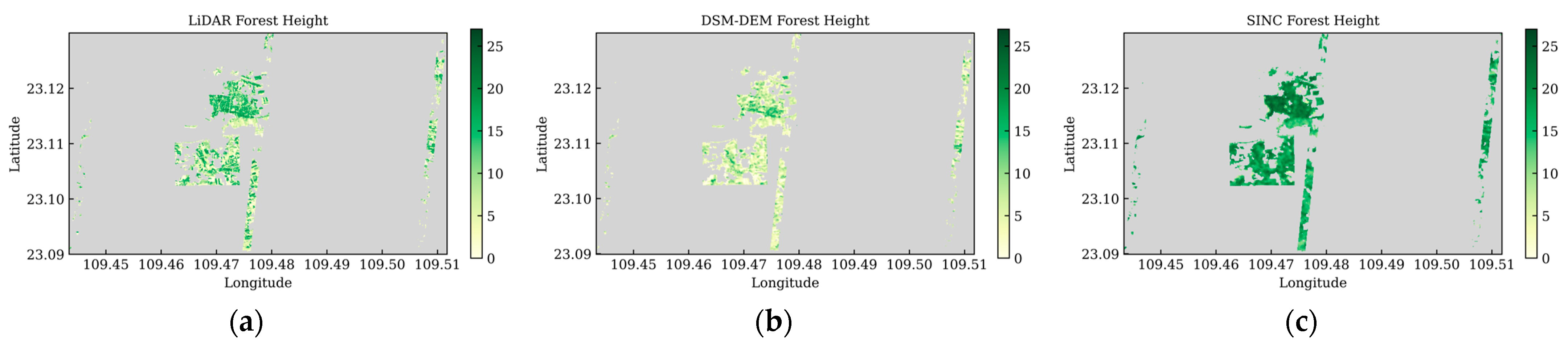
2.3.1. DSM-DEM Differencing Method

The basic workflow of the DSM-DEM differencing method is as follows:

(1)

Extract a DSM from InSAR data, which includes vegetation height.

(2)

Obtain a high-precision DEM from LiDAR data.

(3)

Co-register InSAR DSM and LiDAR DEM to the same coordinate system. Subtract the LiDAR DEM from the InSAR DSM to obtain forest height.

$$h_{phase}=DS{M}_{InSAR}-DE{M}_{LiDAR}$$

(1)

2.3.2. SINC Function Modeling Method

Random Volume over Ground (RVoG) has been widely applied in the estimation of forest height. This model establishes an effective correlation between InSAR observations and forest biophysical parameters. In the RVoG model, the observed coherence $\tilde{\gamma }\left(\omega \right)$ is represented as [35,36]:

$$\tilde{\gamma }\left(\omega \right)=e^{i{\phi }_0}\frac{{\gamma }_v+\mu \left(\omega \right)}{1+\mu \left(\omega \right)}$$

(2)

$${\gamma }_v=\frac{{\displaystyle {\int }_0^{h_v}f\left(z\right)e^{i{k}_{z}z}dz}}{{\displaystyle {\int }_0^{h_v}f\left(z\right)dz}};f\left(z\right)=e^{2\sigma z/\cos \theta }$$

(3)

$$k_z=\frac{2d\pi \Delta \theta }{\lambda \sin \theta }=\frac{2d\pi B_{\perp }}{\lambda R\sin \theta }$$

(4)

In the equation, $f\left(z\right)$ represents the vertical structure function that characterizes the medium scattering contribution. $\mu$ is the ground amplitude ratio, which is dependent on the polarization mode $\omega$. ${\phi }_0$ is the surface phase. $\sigma$ is the extinction coefficient. $h_v$ is the height of the scattering object, specifically the tree height. $\theta$ is the angle of incidence of the electromagnetic wave signal. $\Delta \theta$ represents the difference in incidence angles of the interferometric image. $\lambda$ is the radar wavelength. $R$ is the slant range. $B_{\perp }$ is the vertical baseline. $k_z$ is the effective vertical wave number [37]. In the single-site mode, d = 2, while in the dual-site mode, d = 1.

The observation information from single-baseline, single-polarization data is insufficient to support the solution of the RVoG model for forest height estimation. When the contribution of surface scattering in the X-band and forest-covered areas is neglected $\left(\mu \approx 0\right)$, the observed coherence represents the decorrelation of volume scattering ${\gamma }_v$. Additionally, assuming the extinction coefficient $\sigma$ in the forest region tends to be zero, the decorrelation of volume scattering becomes solely a function of forest height $h_v$. This model is known as the SINC function model, which is substituted into $HoA=2\pi /k_z$, where $HoA$ represents the height of ambiguity, characterizing the height sensitivity of the InSAR signal. The expression for the SINC function model is as follows [14,15]:

$$\left|{\gamma }_v\right|=SINC\left(\frac{\pi h_v}{HoA}\right)$$

(5)

The derived criterion for single-baseline TerraSAR-X/TanDEM-X InSAR coherence-based forest height estimation is as follows:

$$h_v=\frac{HoA}{\pi }\left(\pi -2\arcsin {\left|{\gamma }_v\right|}^{0.8}\right)$$

(6)

Owing to the lack of temporal baseline in the TerraSAR-X/TanDEM-X system, and the acquired SLC data being pre-processed with sub-pixel registration and range-azimuth spectrum filtering, the non-volumetric scattering in the data has been decorrelated, leaving only the ${\gamma }_{SNR}$ component [38,39,40,41]. After correction, the corrected value ${\gamma }_{\nu }$ can be obtained.

$${\gamma }_{SNR}=\frac{1}{\sqrt{1+SN{R}_{TDX}^{-1}}\sqrt{1+SN{R}_{TSX}^{-1}}}$$

(7)

$${\gamma }_{\nu }=\frac{\gamma }{{\gamma }_{SNR}}$$

(8)

In Equation (7): $SN{R}_{TDX}$ and $SN{R}_{TSX}$ represent the signal-to-noise ratio levels of the two satellites, which can be obtained from the header files.

In real-world scenarios, forests are often located in areas with varying terrains. In such cases, the propagation path of electromagnetic waves in forest scatterers is affected by the changes in the terrain, requiring an improved model for forest height inversion in hilly regions. By utilizing an external digital elevation model (DEM), the local correction of the incidence angle can be calculated for computing forest heights across the entire region. This correction is performed by evaluating the local $k_z$ based on Equation (9).

$$k_z^{\prime }=\frac{k_z\sin \theta }{\sin {\theta }^{\prime }}$$

(9)

where $\theta \prime =\theta -\alpha$.

2.3.3. Machine Learning Algorithms

(1)

CART: The CART algorithm involves splitting the sample into two smaller samples, where each non-leaf node in the tree has two branches. It is a binary recursive partitioning technique that can be used for both regression and classification tasks. The resulting tree is referred to as a regression tree [42]. The CART algorithm uses binary splitting to handle continuous data, and it selects features and performs splits based on minimizing the squared error criterion. In addition to the general advantages of decision tree models, such as simplicity and high accuracy, CART algorithm does not impose any requirements on the probability distribution of the target and predictor variables. It can also handle missing values, thus reducing bias caused by missing data [43,44]. In this study, the CART algorithm was implemented on the GEE cloud platform. The default values are null for maxNodes and 1 for minLeafPopulation.

(2)

GBDT: GBDT is a boosting algorithm for ensemble learning proposed by Friedman [45]. Its training process is conducted in a sequential manner, where the training of weak learners is ordered. Each weak learner learns based on the previous learner’s performance. GBDT typically uses decision trees as the base weak classifiers. The main idea behind GBDT is that each decision tree is constructed along the gradient direction of the previously built residual reduction. In other words, each new tree is built to reduce the residual of all previous trees in the direction of the gradient. This algorithm obtains a decision tree at each training iteration, and the trained decision trees are iteratively combined to form a strong learner [46,47,48,49]. In this study, the GBDT algorithm was implemented on the GEE cloud platform. Through iterative experiments, the following specific parameter settings were found: ntree = 160, shrinkage = 0.07.

(3)

RF: RF is a tree-based algorithm composed of many decision trees or regression trees, where each tree relies on the values of randomly sampled vectors and all trees have the same distribution in the data [50,51,52,53]. When using the RF algorithm on the GEE platform, only two parameters need to be set: the number of trees to generate (ntree) and the number of inverse variables used to split each node (Mtry). Through iterative experiments, ntree was set to 220 to avoid overfitting while ensuring accuracy. Mtry was configured with the default setting, which corresponds to the square root of the input feature variables’ number. The default value of null was assigned to maxNodes, while the default value of 1 was assigned to minLeafPopulation.

(4)

SVM: SVM is a novel algorithm based on statistical theory proposed by Vapnik. It is commonly used for small-sample nonlinear problems [54]. The principle can be understood as extending linearly inseparable data into a multidimensional space and using hyperplanes for classification. By finding the minimum structured risk, it enhances the generalization ability of feature combinations, thereby achieving the goal of obtaining effective statistical patterns even with limited statistical samples [55,56,57,58]. In this study, the implementation of the SVM algorithm was done on the GEE cloud platform. For the parameter settings of the SVM algorithm, the widely recognized radial basis function is used as the SVM’s kernel function.

2.3.4. Feature Combination and Performance Evaluation

To evaluate the ability to estimate forest height using interferometric, backscatter coefficient, and local incidence angle information, three feature combinations were established: Feature Combination A (FC_A), Feature Combination B (FC_B), and Feature Combination C (FC_C). The variation in local incidence angle can influence the intensity of backscatter coefficient. Therefore, in the subsequent sections, we combine backscatter coefficients and local incidence angles as a set of features. The variable feature set consists of coherence, decorrelation of volume scattering, backscatter coefficient, local incidence angle, fraction of vegetation cover, slope, aspect, and elevation. The three feature combinations are summarized in

Table 3. Feature combinations of interferometric, backscatter coefficient, and local incidence angle information.

Feature Combination	Features
A	Interferometric features (coherence, decorrelation of volume scattering)
	Spectral features (fraction of vegetation cover)
	Topographic features (slope, aspect, elevation)
B	(backscatter coefficient, local incidence angle)
	Spectral features (fraction of vegetation cover)
	Topographic features (slope, aspect, elevation)
C	Interferometric features (coherence, decorrelation of volume scattering)
	(backscatter coefficient, local incidence angle)
	Spectral features (fraction of vegetation cover)
	Topographic features (slope, aspect, elevation)

.

To assess the accuracy of forest height estimation, the following procedures were carried out on the GEE platform: randomColumn() was employed to add a random attribute to the sample points, and the sample point data were randomly divided into two groups: 80% of the sample points were used for training, while the remaining 20% were used for validation. The coefficient of determination (R²) and root mean square error (RMSE) were used to evaluate the accuracy of the feature combinations.

3. Results

3.1. Validation of Forest Height Estimation Accuracy

In order to assess the impact of different methods on forest height estimation, the following analysis is conducted on the results of forest height estimation using the DSM-DEM differencing method, the SINC function modeling method, feature combinations A, B, and C. Figure 4 and Figure 5 display the forest height obtained from LiDAR data, the DSM-DEM differencing method, and the SINC function modeling method. Figure 6, Figure 7, Figure 8, Figure 9, Figure 10 and Figure 11 display the forest height predicted by regression using different feature combinations and algorithms.

3.1.1. DSM-DEM Differencing Method and SINC Function Modeling Method

Figure 4b,c respectively depict the forest height estimated by the DSM-DEM differencing method and the SINC function modeling method. The DSM-DEM differencing method exhibits a certain degree of underestimation in forest height estimation, while the SINC function modeling method shows a noticeable overestimation. The forest height distribution acquired through the DSM-DEM differencing method aligns more accurately with the LiDAR forest height in terms of details.

Figure 5 presents the validation scatter plots for the DSM-DEM differencing method and the SINC function modeling method, with R² values of 0.38 and 0.23, respectively. The corresponding RMSE values are 4.34 m and 11.43 m. Both methods yield unsatisfactory estimation results. The scatter plot of the DSM-DEM differencing method appears more dispersed compared to the SINC function modeling method, and the underestimation becomes more evident as the forest height increases. The scatter plot of the SINC function modeling method appears relatively concentrated, but it exhibits significant overestimation at lower forest heights, resulting in a larger deviation from the LiDAR forest height.

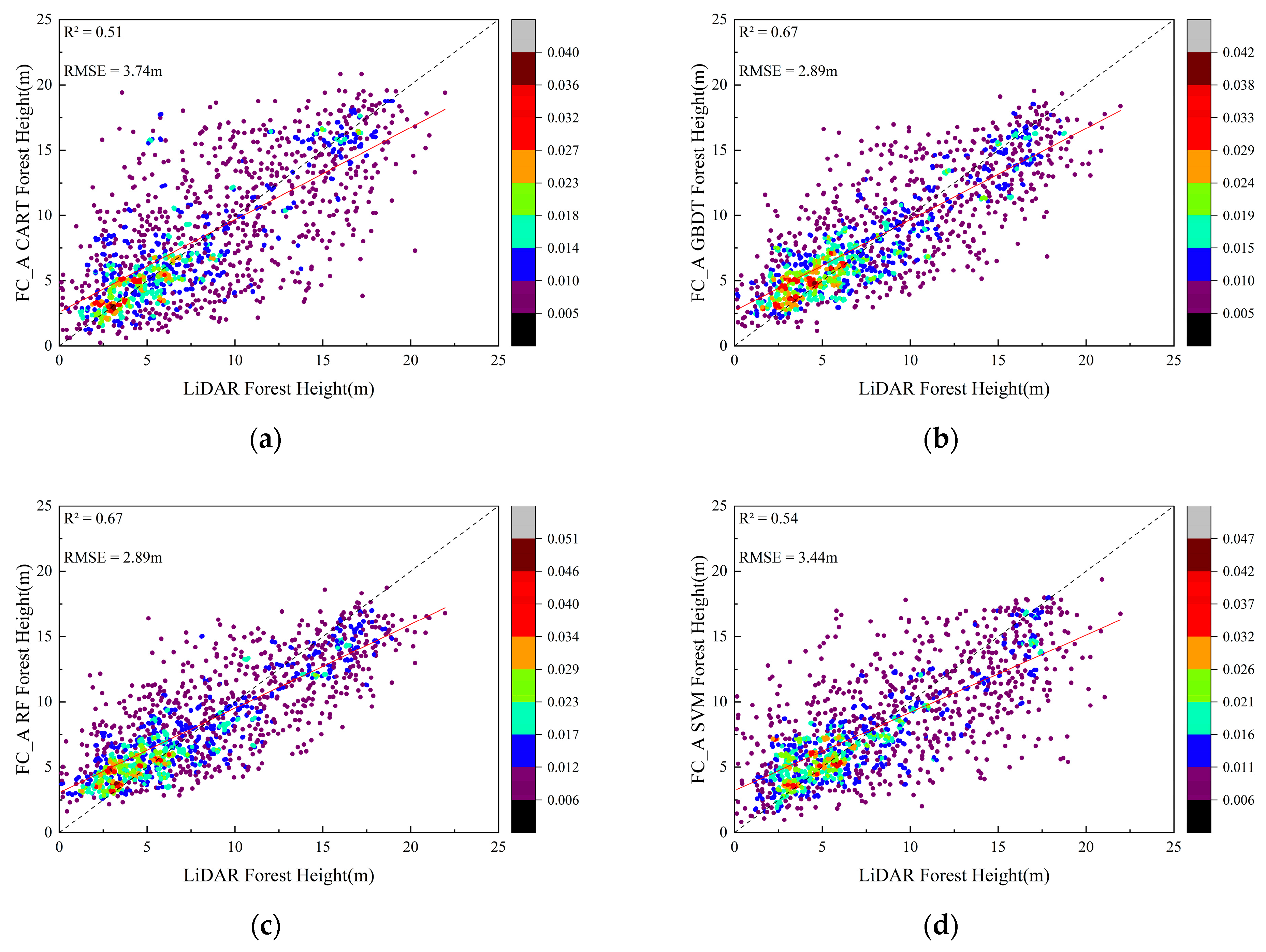
3.1.2. Feature Combination A

Figure 6 presents the forest height estimated by the CART, GBDT, RF, and SVM algorithms for feature combination A. The four forest height estimation results show good consistency with LiDAR-derived forest height. Among them, the forest height distribution estimated by the CART algorithm is closest to the LiDAR-derived forest height, while the RF algorithm exhibits significant underestimation compared to LiDAR-derived forest height. All algorithms exhibit varying degrees of underestimation in their estimation results.

Figure 7 displays the validation scatter plots for each algorithm. Overall, the forest height estimation accuracy is relatively good, with R² values of 0.51, 0.67, 0.67, and 0.54 for CART, GBDT, RF, and SVM algorithms, respectively. The corresponding RMSE values are 3.74 m, 2.89 m, 2.89 m, and 3.44 m. The scatter plot of the CART algorithm shows more scattering compared to the other three machine learning algorithms. GBDT and RF algorithms perform well in estimating the heights of low trees (0–7.5 m) and medium to high trees (15 m and above), while all machine learning algorithms exhibit some scattering in the estimation results for trees ranging from 7.5 m to 15 m. A certain overestimation is observed when LiDAR-derived forest height is close to 0 m, and as LiDAR-derived forest height increases, the underestimation becomes more pronounced for all machine learning algorithms. In general, GBDT and RF algorithms demonstrate better estimation accuracy, while the CART algorithm shows poorer estimation results.

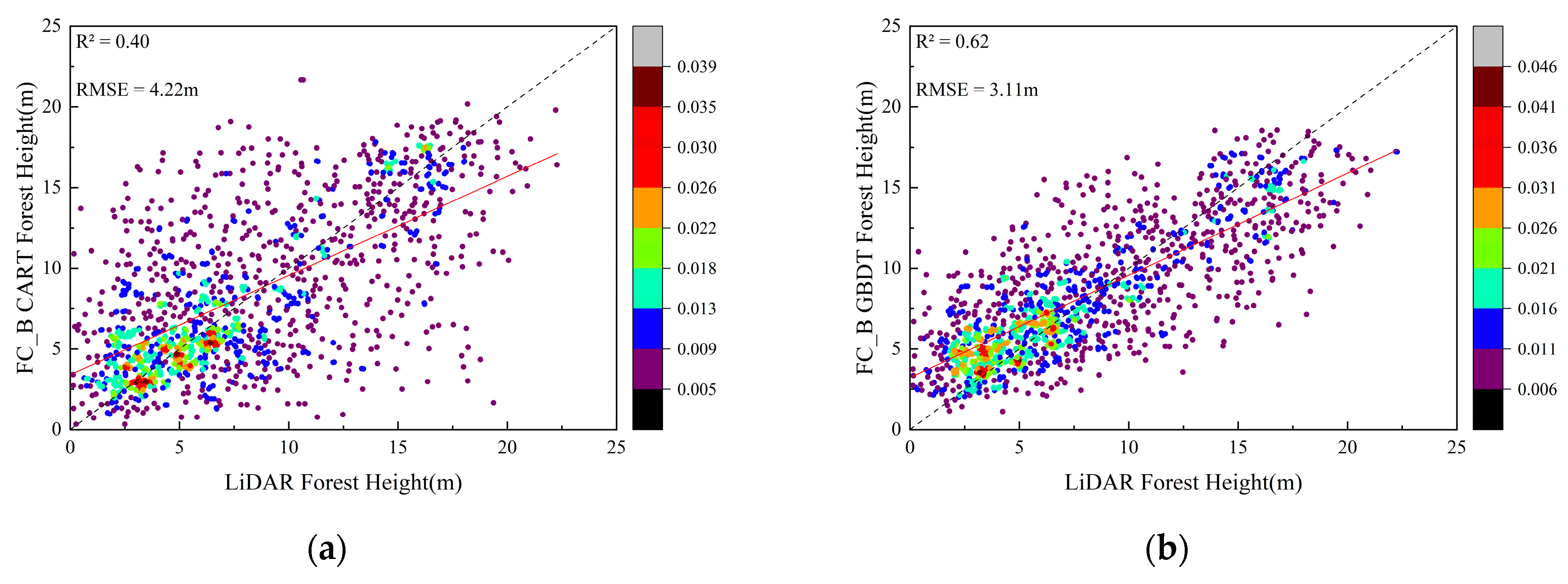
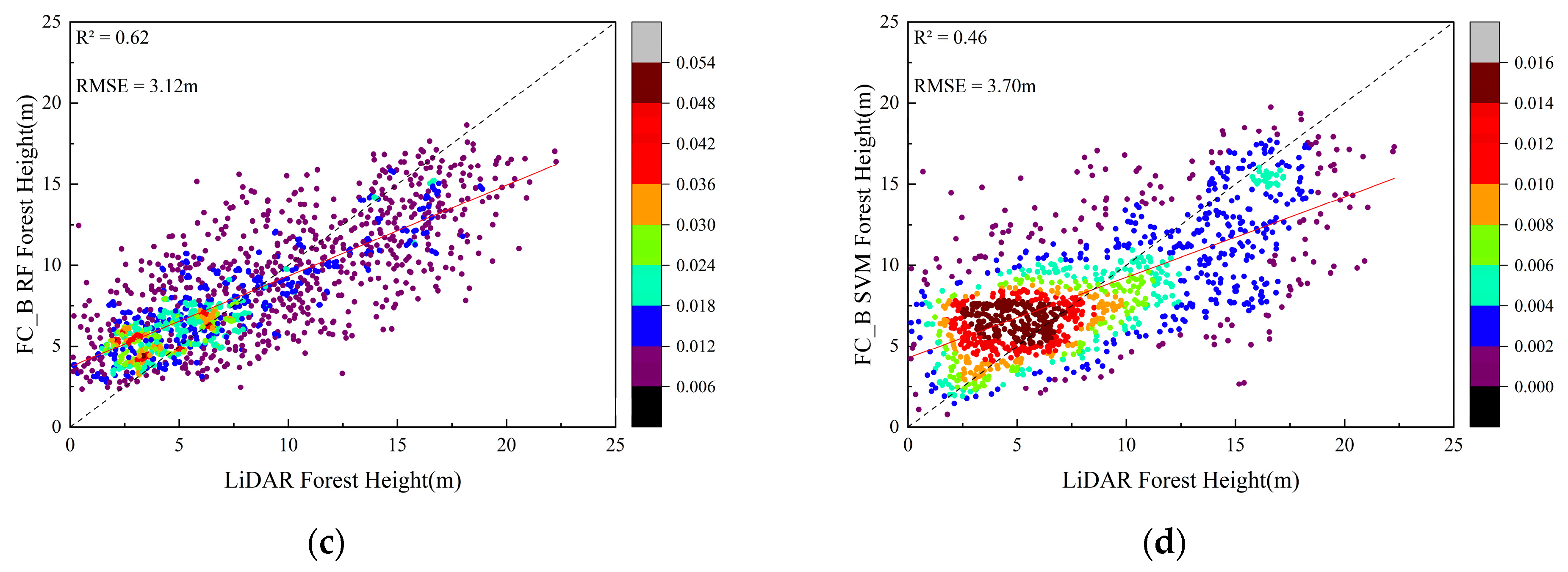
3.1.3. Feature Combination B

Figure 8 displays the estimated forest height using different algorithms for feature combination B. It can be observed that the forest height distribution estimated by the CART algorithm is closest to the LiDAR forest height, while the RF algorithm consistently underestimates the forest height compared to LiDAR measurements. All algorithms exhibit varying degrees of underestimation in their estimations.

Figure 9 presents the validation scatter plots for each algorithm. The R² values for CART, GBDT, RF, and SVM algorithms are 0.40, 0.62, 0.62, and 0.46, respectively. The corresponding RMSE values are 4.22 m, 3.11 m, 3.12 m, and 3.70 m. Compared to feature combination A, the accuracy of forest height estimation decreases when using feature combination B with different machine learning algorithms. Specifically, the CART and SVM algorithms show a significant decrease in accuracy, with R² decreasing by 0.11 and 0.08, respectively, and RMSE increasing by 0.48 m and 0.26 m, respectively. The scatter plot of the CART algorithm exhibits a greater dispersion compared to feature combination A, while the scatter plot of the SVM algorithm is concentrated in the range of shorter trees with a noticeable overestimation. In the range of medium to tall trees, all machine learning algorithms exhibit underestimation. Overall, the GBDT and RF algorithms demonstrate better accuracy in forest height estimation, while the CART and SVM algorithms perform relatively poorly.

3.1.4. Feature Combination C

Figure 10 presents the estimated forest height for feature combination C using different algorithms, and the validation scatter plots for each algorithm are shown in Figure 11. The R² values for CART, GBDT, RF, and SVM algorithms are 0.43, 0.65, 0.63, and 0.49, respectively. The corresponding RMSE values are 4.10 m, 2.91 m, 2.99 m, and 3.55 m.

From the different feature combinations, it can be observed that when estimating forest height, using feature combination B alone results in the poorest accuracy. The accuracy improves when combining backscatter coefficient, local incidence angle with interferometric information (feature combination C), compared to feature combination B alone. Compared to interferometric information alone (feature combination A), feature combinations A and C show similar accuracy when using the GBDT and RF algorithms (RMSE increases by no more than 10 cm). However, when using the CART and SVM algorithms, feature combination A performs significantly better than feature combination C in terms of estimation accuracy.

Generally, when inverting forest parameters, various machine learning algorithms are utilized to ascertain the capability of these algorithms in estimating forest height based on interferometric, backscatter coefficient, and local incidence angle data. The aim is not only to compare the performance of different algorithms but also to illustrate that interferometric, backscatter coefficient, and local incidence angle information can be effectively employed for forest height estimation, independent of any specific algorithm.

3.2. Large-Scale Forest Height Mapping

Based on the comprehensive analysis above, the machine learning algorithm exhibits higher estimation accuracy compared to the DSM-DEM differencing method and the SINC function modeling method. Among the feature combinations A, B, and C, the GBDT algorithm consistently produces the best forest height estimation results (with the RF algorithm demonstrating similar estimation accuracy with feature combination A). In this study, the merging of combination A and the GBDT algorithm was employed to generate a spatial distribution map of forest heights from SAR imagery (Figure 12a). It can be observed that different forest stands exhibit significant spatial variability across the image.

Figure 12b,c present a comparison between selected representative regions from Figure 12a and optical remote sensing imagery from Google Earth, respectively. Figure 12b is located in a mountainous area, where two distinct bare areas are visible (indicating forest heights of 0 m). It can be noted that the forest height estimates obtained using the merging of combination A and the GBDT algorithm closely approximate zero in these two areas. This suggests that the merging of combination A and the GBDT algorithm provides the ability to discriminate land features and estimate forest heights in areas not included in the training dataset. Figure 12c is situated near a lake and predominantly consists of regularly shaped plantation forests. The forest height estimates and contours derived from the merging of combination A and the GBDT algorithm closely resemble the characteristics of the plantation forests, thereby demonstrating the effectiveness of this method.

4. Discussion

4.1. Deviation in Forest Height Estimation

Compared to the DSM-DEM differencing method and the SINC function modeling method, the forest height estimates from various machine learning algorithms outperform these two conventional methods in terms of accuracy. In order to better compare the forest height results obtained from different methods, height difference maps (Figure 13) were generated by subtracting the forest height estimates from each method with LiDAR-derived forest height.

In the DSM-DEM differencing method, a phenomenon of height underestimation is evident (with 66% of the height differences being negative), indicating a certain penetration capability of the X-band in the forest canopy. In the SINC function modeling method, a phenomenon of height overestimation is more pronounced (with 94% of the height differences being positive), suggesting that the SINC function modeling method may not accurately capture the spatial distribution characteristics of tree branches and canopies when applied to trees with specific shapes, such as eucalyptus trees (which are dominant species in the study area).

In feature combination A, similar proportions of height underestimation and overestimation are observed across all algorithms (approximately −19 to +15 m). In feature combinations B and C, the extent of height underestimation and overestimation increases for the RF and SVM algorithms, while the CART and GBDT algorithms exhibit smaller variations in height underestimation and overestimation. Among the feature combinations A, B, and C, the GBDT algorithm shows the smallest height difference compared to LiDAR-derived forest height, indicating that it not only exhibits the best consistency with LiDAR-derived forest height, but also has the smallest height deviation.

Since the training samples mostly come from the 0–10 m and 10–20 m height ranges, with few samples near 0 m or in the 20–30 m range (due to non-proportional sampling according to the distribution range of LiDAR-derived forest height in the study area), all algorithms achieve effective estimates within the 0–20 m height range. However, they tend to overestimate the forest height near 0 m and underestimate it significantly in the 20–30 m range compared to LiDAR-derived forest height. This indicates that the performance of algorithms depends on the input of training samples. It is advisable to select sample sites with consistent sample sizes across different height ranges and densities to mitigate overestimation or underestimation effects of algorithms and achieve better estimation results.

4.2. Comparison of Forest Height Estimation Methods

In the subtropical region, when eucalyptus trees are dominant species, the DSM-DEM differencing method and the SINC function modeling method exhibit significant deviations from the actual forest height. However, combining interferometric information, backscatter coefficient, local incidence angle information, and machine learning algorithms yielded better results (

Table 4. Comparison of forest height estimation performance between DSM-DEM and SINC.

	DSM-DEM	SINC
R2	0.38	0.23
RMSE (m)	4.34	11.43

and

Table 5. Comparison of forest height estimation performance using different feature combinations and machine learning algorithms.

Feature Combination	CART		GBDT		RF		SVM
	R2	RMSE (m)	R2	RMSE (m)	R2	RMSE (m)	R2	RMSE (m)
A	0.51	3.74	0.67	2.89	0.67	2.89	0.54	3.44
B	0.40	4.22	0.62	3.11	0.62	3.12	0.46	3.70
C	0.43	4.10	0.65	2.91	0.63	2.99	0.49	3.55

).

The DSM-DEM differencing method tends to underestimate the forest height to some extent. Despite the X-band being a short-wave SAR band, it still exhibits certain penetration capabilities for the forest canopy. The estimated height obtained by this method represents the height of the effective scattering center, which is lower than the actual forest height.

The SINC function modeling method shows the largest deviation in estimation results. The reasons for this could be as follows: Eucalyptus trees typically have large horizontal canopy areas, exhibiting a flat or expanded shape. This broad canopy shape may result in multiple scattering events within the canopy, making it difficult for the SINC function modeling method to accurately distinguish the contributions of different scattering processes. This may lead to an overestimation of tree height by the model, since it cannot accurately explain the reflection and scattering processes within the canopy. Additionally, variations in cloud cover, precipitation, and atmospheric humidity, as well as instrument errors, electromagnetic interference, and signal attenuation during transmission in the subtropical region, may cause attenuation or scattering of radar signals, leading to a decrease in the coherence quality of the image. The SINC function modeling method has higher requirements in terms of data quality. In such cases, forest height estimation based on the SINC function modeling method may not yield satisfactory results.

TerraSAR-X/TanDEM-X provides coherence, decorrelation of volume scattering, backscatter coefficient, and local incidence angle. They are used to establish combinations of features for forest height estimation (feature combination A, feature combination B, and feature combination C). This allows the effective comparison of the strengths and weaknesses of interferometric, backscatter coefficient, and local incidence angle information in estimating forest height. When using feature combinations A and B as feature datasets, the former four machine learning algorithms achieved higher R² values and lower RMSE values, whereas the latter achieved lower R² values and higher RMSE values. When estimating forest height using feature combination C, the accuracy improved for feature combination B, while the accuracy of feature combination A did not improve, and even decreased, indicating that interferometric information has better estimation effects compared to backscatter coefficient, local incidence angle information.

When trees have uneven distributions of branches and trunks, as well as complex architectural and hierarchical structures, combining interferometric information, backscatter coefficient, local incidence angle information, and machine learning algorithms can achieve better results in estimating forest height.

4.3. Machine Learning Algorithm Variable Analysis

In order to assess the sensitivity of input features on forest height estimation, in this study, an analysis of feature importance was conducted (Figure 14). It can be observed that the sensitivity of input features varies across different feature combinations. Based on their importance ranking, the four most important features in each feature combination using the RF algorithm are as follows:

Feature Combination A: Fraction of vegetation cover, coherence, decorrelation of volume scattering, elevation.

Feature Combination B: Fraction of vegetation cover, backscatter coefficient, elevation, local incidence angle.

Feature Combination C: Fraction of vegetation cover, coherence, backscatter coefficient, decorrelation of volume scattering.

It can be seen that fraction of vegetation cover is the most significant factor influencing forest height estimation in all feature combinations, followed by interferometric, backscatter coefficient, and local incidence angle information. Terrain slope and aspect have a relatively smaller impact on forest height estimation.

Many studies have found that forest height estimation is influenced by terrain factors. In regions with significant topographic variations, changes in local incidence angle cause variations in effective vertical wavenumber and height ambiguity, thereby affecting forest height estimation [18,19]. In this study, the influence of terrain factors on forest height estimation is relatively small, due to the limited topographic variations in the study area. However, this influence should not be completely ignored.

In addition to terrain features, this study also incorporates spectral features (fraction of vegetation cover). Previous research has shown that fraction of vegetation cover affects the penetration depth of the X-band through the forest canopy, and there is a certain correlation between forest height and penetration depth, thus impacting forest height estimation. In this study, fraction of vegetation cover has a significant impact on forest height estimation due to the presence of different tree species in the study area, each with varying crown shapes and densities. Fraction of vegetation cover also varies within the same tree species due to differences in tree age and spacing. Therefore, the roles of terrain features and spectral features in forest height estimation should not be overlooked.

4.4. Limitations and Prospects

The TerraSAR-X/TanDEM-X data applied in this study were acquired using a single baseline and single polarization, which is the primary data acquisition mode of the current TerraSAR-X/TanDEM-X system. Compared to multi-baseline and full-polarization data, single-baseline and single-polarization data provide limited information, thus limiting the analysis of more comprehensive interferometric and polarization information.

Machine learning regression inversion methods are often regarded as black box models, and their results may lack interpretability of the physical processes. In future research, the interpretability of machine learning can be improved by selecting relevant features to the research question, employing machine learning models with high interpretability, and utilizing visualization methods to present the results of the models.

When airborne LiDAR data point cloud density is low, it can pose challenges in generating DSM and DEM through point cloud processing. Typically, interpolation methods are employed to estimate the values of DSM and DEM for sparse point cloud grid cells. Furthermore, using airborne LiDAR forest height data as a reference has certain limitations, as LiDAR-derived forest height is also subject to inherent errors during computation. In future research, it is advisable to utilize forest inventory data specific to the study year or ground measurement data from selected sample plots whenever possible [59,60].

5. Conclusions

This study provides evaluates the performance of forest height estimation using various algorithms, including CART, GBDT, RF, and SVM, with TerraSAR-X/TanDEM-X data as the primary data source. The main conclusions are as follows:

(1)

The estimation accuracy of different feature combinations and machine learning algorithms is superior to DSM-DEM differencing and SINC function modeling methods.

(2)

Modeling based on interferometric information demonstrates better estimation accuracy compared to modeling based on backscatter coefficient, local incidence angle information, or a combination of interferometric information and backscatter coefficient and local incidence angle information across all machine learning algorithms.

(3)

GBDT and RF algorithms both achieve accurate forest height estimation. GBDT exhibits higher precision, with R² values of 0.67, 0.62, and 0.65, and corresponding RMSE values of 2.89 m, 3.11 m, and 2.91 m for feature combinations A, B, and C, respectively.

(4)

Interferometric information combined with machine learning algorithms has great potential in forest height estimation. The method proposed in this study allows the cost-effective estimation of forest height over large areas.

References

1. Vatandaslar, C.; Narin, O.G.; Abdikan, S. Retrieval of forest height information using spaceborne LiDAR data: A comparison of GEDI and ICESat-2 missions for Crimean pine (Pinus nigra) stands. Trees 2023, 37, 717–731. [Google Scholar] [CrossRef]
2. Chen, E.; Li, Z.; Pang, Y.; Tian, X. Average tree height extraction technique based on polarimetric synthetic aperture radar interferometry. For. Sci. 2007, 66–70+145. [Google Scholar]
3. Pan, Y.; Birdsey, R.A.; Fang, J.; Houghton, R.; Kauppi, P.E.; Kurz, W.A.; Phillips, O.L.; Shvidenko, A.; Lewis, S.L.; Canadell, J.G.; et al. A large and persistent carbon sink in the world’s forests. Science 2011, 333, 988–993. [Google Scholar] [CrossRef] [PubMed]
4. Nikhil, S.; Danumah, J.H.; Saha, S.; Prasad, M.K.; Rajaneesh, A.; Mammen, P.C.; Ajin, R.S.; Kuriakose, S.L. Application of GIS and AHP method in forest fire risk zone mapping: A study of the Parambikulam tiger reserve, Kerala, India. J. Geovis. Spat. Anal. 2021, 5, 14. [Google Scholar] [CrossRef]
5. Amrutha, K.; Danumah, J.H.; Nikhil, S.; Saha, S.; Rajaneesh, A.; Mammen, P.C.; Ajin, R.S.; Kuriakose, S.L. Demarcation of forest fire risk zones in Silent Valley National Park and the effectiveness of forest management regime. J. Geovis. Spat. Anal. 2022, 6, 8. [Google Scholar] [CrossRef]
6. Wang, Y.; Lehtomäki, M.; Liang, X.; Pyörälä, J.; Kukko, A.; Jaakkola, A.; Liu, J.; Feng, Z.; Chen, R.; Hyyppä, J. Is field-measured tree height as reliable as believed–A comparison study of tree height estimates from field measurement, airborne laser scanning and terrestrial laser scanning in a boreal forest. ISPRS J. Photogramm. Remote Sens. 2019, 147, 132–145. [Google Scholar] [CrossRef]
7. Persson, H.J.; Ståhl, G. Characterizing uncertainty in forest remote sensing studies. Remote Sens. 2020, 12, 505. [Google Scholar] [CrossRef]
8. Fassnacht, F.E.; White, J.C.; Wulder, M.A.; Næsset, E. Remote sensing in forestry: Current challenges, considerations and directions. For. Int. J. For. Res. 2023, cpad024. [Google Scholar] [CrossRef]
9. Rodriguez, E.; Martin, J.M. Theory and design of interferometric synthetic aperture radars. In IEE Proceedings F (Radar and Signal Processing); IET Digital Library: Londone, UK, 1992; Volume 139, pp. 147–159. [Google Scholar]
10. Li, L.; Chen, E.; Li, Z.; Feng, Q.; Zhao, L. A Review on Forest Height and Above-ground Biomass Estimation based on Synthetic Aperture Radar. Remote Sens. Technol. Appl. 2016, 31, 625. [Google Scholar] [CrossRef]
11. Zhang, H.; Wang, C.; Zhu, J.; Fu, H.; Xie, Q.; Shen, P. Forest above-ground biomass estimation using single-baseline polarization coherence tomography with P-band PolInSAR data. Forests 2018, 9, 163. [Google Scholar] [CrossRef]
12. Soja, M.J.; Ulander, L.M. Digital canopy model estimation from TanDEM-X interferometry using high-resolution lidar DEM. In Proceedings of the 2013 IEEE International Geoscience and Remote Sensing Symposium-IGARSS, Melbourne, VIC, Australia, 21–26 July 2013; pp. 165–168. [Google Scholar]
13. Sadeghi, Y.; St-Onge, B.; Leblon, B.; Simard, M.; Papathanassiou, K. Mapping forest canopy height using TanDEM-X DSM and airborne LiDAR DTM. In Proceedings of the 2014 IEEE Geoscience and Remote Sensing Symposium, Quebec City, QC, Canada, 13–18 July 2014; pp. 76–79. [Google Scholar]
14. Cloude, S. Polarisation: Applications in Remote Sensing; OUP Oxford: Oxford, UK, 2009. [Google Scholar]
15. Cloude, S.R.; Chen, H.; Goodenough, D.G. Forest height estimation and validation using Tandem-X polinsar. In Proceedings of the 2013 IEEE International Geoscience and Remote Sensing Symposium-IGARSS, Melbourne, VIC, Australia, 21–26 July 2013; pp. 1889–1892. [Google Scholar]
16. Feng, Q.; Chen, E.; Li, Z.; Li, L.; Zhao, L. Forest Height Estimation from Airborne X-band Single-pass InSAR Data. Remote Sens. Technol. Appl. 2016, 31, 551–557. [Google Scholar]
17. Caicoya, A.T.; Kugler, F.; Hajnsek, I.; Papathanassiou, K.P. Large-scale biomass classification in boreal forests with TanDEM-X data. IEEE Trans. Geosci. Remote Sens. 2016, 54, 5935–5951. [Google Scholar] [CrossRef]
18. Fan, Y.; Chen, E.; Li, Z.; Zhao, L.; Zhang, W.; Jin, Y.; Cai, L. Forest Height Estimation Method Using TanDEM-X Interferometric Coherence Data. For. Sci. 2020, 56, 35–46. [Google Scholar]
19. Zhang, T.; Zhu, J.; Fu, H.; Wang, C. Forest height inversion with single-baseline TanDEM-X InSAR coherence. Acta Geod. Cartogr. Sin. 2022, 51, 1931–1941. [Google Scholar]
20. Wang, H.; Zhao, Y.; Pu, R.; Zhang, Z. Mapping Robinia pseudoacacia forest health conditions by using combined spectral, spatial, and textural information extracted from IKONOS imagery and random forest classifier. Remote Sens. 2015, 7, 9020–9044. [Google Scholar] [CrossRef]
21. Zhao, J.; Zhang, Z.; Han, S.; Qu, C.; Yuan, Z.; Zhang, D. SVM based forest fire detection using static and dynamic features. Comput. Sci. Inf. Syst. 2011, 8, 821–841. [Google Scholar] [CrossRef]
22. Singh, S.K.; Srivastava, P.K.; Gupta, M.; Thakur, J.K. Mukherjee, S. Appraisal of land use/land cover of mangrove forest ecosystem using support vector machine. Environ. Earth Sci. 2014, 71, 2245–2255. [Google Scholar] [CrossRef]
23. Fassnacht, F.E.; Hartig, F.; Latifi, H.; Berger, C.; Hernández, J.; Corvalán, P.; Koch, B. Importance of sample size, data type and prediction method for remote sensing-based estimations of aboveground forest biomass. Remote Sens. Environ. 2014, 154, 102–114. [Google Scholar] [CrossRef]
24. Chen, G.; Hay, G.J.; St-Onge, B. A GEOBIA framework to estimate forest parameters from lidar transects, Quickbird imagery and machine learning: A case study in Quebec, Canada. Int. J. Appl. Earth Obs. Geoinform. 2012, 15, 28–37. [Google Scholar] [CrossRef]
25. Gu, C.; Clevers, J.G.; Liu, X.; Tian, X.; Li, Z.; Li, Z. Predicting forest height using the GOST, Landsat 7 ETM+, and airborne LiDAR for sloping terrains in the Greater Khingan Mountains of China. ISPRS J. Photogramm. Remote Sens. 2018, 137, 97–111. [Google Scholar] [CrossRef]
26. García, M.; Saatchi, S.; Ustin, S.; Balzter, H. Modelling forest canopy height by integrating airborne LiDAR samples with satellite Radar and multispectral imagery. Int. J. Appl. Earth Obs. Geoinf. 2018, 66, 159–173. [Google Scholar] [CrossRef]
27. Li, W.; Niu, Z.; Shang, R.; Qin, Y.; Wang, L.; Chen, H. High-resolution mapping of forest canopy height using machine learning by coupling ICESat-2 LiDAR with Sentinel-1, Sentinel-2 and Landsat-8 data. Int. J. Appl. Earth Obs. Geoinf. 2020, 92, 102163. [Google Scholar] [CrossRef]
28. Brigot, G.; Simard, M.; Colin-Koeniguer, E.; Boulch, A. Retrieval of forest vertical structure from PolInSAR data by machine learning using LIDAR-derived features. Remote Sens. 2019, 11, 381. [Google Scholar] [CrossRef]
29. Xie, Y.; Fu, H.; Zhu, J.; Wang, C.; Xie, Q. A LiDAR-aided multibaseline PolInSAR method for forest height estimation: With emphasis on dual-baseline selection. IEEE Geosci. Remote Sens. Lett. 2019, 17, 1807–1811. [Google Scholar] [CrossRef]
30. Pourshamsi, M.; Garcia, M.; Lavalle, M.; Balzter, H. A machine-learning approach to PolInSAR and LiDAR data fusion for improved tropical forest canopy height estimation using NASA AfriSAR Campaign data. IEEE J. Sel. Top. Appl. Earth Obs. Remote Sens. 2018, 11, 3453–3463. [Google Scholar] [CrossRef]
31. Pourshamsi, M.; Garcia, M.; Lavalle, M.; Pottier, E.; Balzter, H. Machine-learning fusion of PolSAR and LiDAR data for tropical forest canopy height estimation. In Proceedings of the IGARSS 2018–2018 IEEE International Geoscience and Remote Sensing Symposium, Valencia, Spain, 22–27 July 2018; pp. 8108–8111. [Google Scholar]
32. Pourshamsi, M.; Xia, J.; Yokoya, N.; Garcia, M.; Lavalle, M.; Pottier, E.; Balzter, H. Tropical forest canopy height estimation from combined polarimetric SAR and LiDAR using machine-learning. ISPRS J. Photogramm. Remote Sens. 2021, 172, 79–94. [Google Scholar] [CrossRef]
33. Weber, M. TerraSAR-X and TanDEM-X: Reconnaisance applications. In Proceedings of the 2007 3rd International Conference on Recent Advances in Space Technologies, Istanbul, Turkey, 14–16 June 2007; pp. 299–303. [Google Scholar]
34. Krieger, G.; Moreira, A.; Fiedler, H.; Hajnsek, I.; Werner, M.; Younis, M.; Zink, M. TanDEM-X: A satellite formation for high-resolution SAR interferometry. IEEE Trans. Geosci. Remote Sens. 2007, 45, 3317–3341. [Google Scholar] [CrossRef]
35. Papathanassiou, K.P.; Cloude, S.R. Single-baseline polarimetric SAR interferometry. IEEE Trans. Geosci. Remote Sens. 2001, 39, 2352–2363. [Google Scholar] [CrossRef]
36. Cloude, S.R.; Papathanassiou, K.P. Three-stage inversion process for polarimetric SAR interferometry. IEE Proc.-Radar Sonar Navig. 2003, 150, 125–134. [Google Scholar] [CrossRef]
37. Kugler, F.; Lee, S.K.; Hajnsek, I.; Papathanassiou, K.P. Forest height estimation by means of Pol-InSAR data inversion: The role of the vertical wavenumber. IEEE Trans. Geosci. Remote Sens. 2015, 53, 5294–5311. [Google Scholar] [CrossRef]
38. Duque, S.; Balls, U.; Rossi, C.; Fritz, T.; Balzer, W. TanDEM-X. Ground Segment. CoSSC Generation and Interferometric Considerations. Issue: 1.0; Deutsches Zentrum fuer Luft-und Raumfahrt (DLR): Oberpfaffenhofen, Germany, 2012. [Google Scholar]
39. Fritz, T. TanDEM-X. Ground Segment. TanDEM-X Experimental Product Description. Issue: 1.2; Deutsches Zentrum fuer Luft-und Raumfahrt (DLR): Oberpfaffenhofen, Germany, 2012. [Google Scholar]
40. Martone, M.; Bräutigam, B.; Rizzoli, P.; Gonzalez, C.; Bachmann, M.; Krieger, G. Coherence evaluation of TanDEM-X interferometric data. ISPRS J. Photogramm. Remote Sens. 2012, 73, 21–29. [Google Scholar] [CrossRef]
41. Kugler, F.; Schulze, D.; Hajnsek, I.; Pretzsch, H.; Papathanassiou, K.P. TanDEM-X Pol-InSAR performance for forest height estimation. IEEE Trans. Geosci. Remote Sens. 2014, 52, 6404–6422. [Google Scholar] [CrossRef]
42. Dong, H.; Xu, H.; Lu, B.; Yang, Q. A CART-based approach to predict nitrogen oxide concentration along urban traffic roads. Acta Sci. Circumstantiae 2019, 39, 1086–1094. [Google Scholar] [CrossRef]
43. Li, Z.; Du, J.; Zhou, Y. Rainfall prediction model based on improved CART algorithm. Mod. Electron. Tech. 2020, 43, 133–137+141. [Google Scholar] [CrossRef]
44. Guan, Y.; Wang, W.; Liu, S. Building and application of summer high temperature prediction model based on CART algorithm. J. Meteorol. Sci. 2018, 38, 539–544. [Google Scholar]
45. Friedman, J.H. Greedy function approximation: A gradient boosting machine. Ann. Stat. 2001, 29, 1189–1232. [Google Scholar] [CrossRef]
46. Sun, J. Surface Water Information Extraction from High Resolution Remotely Sensed Image Based on Integrated Learning; Jilin University: Jilin, China, 2020. [Google Scholar] [CrossRef]
47. Zhang, W.; Wei, Q.; Wu, T.; Lin, J.; Shao, G.; Ding, M. Prediction models of reference crop evapotranspiration based on gradient boosting decision tree (GBDT) algorithm in Jiangsu province. Jiangsu J. Agric. Sci. 2020, 36, 1169–1180. [Google Scholar]
48. Wu, W.; Wang, J.; Huang, Y.; Zhao, H.; Wang, X. A novel way to determine transient heat flux based on GBDT machine learning algorithm. Int. J. Heat Mass Transf. 2021, 179, 121746. [Google Scholar] [CrossRef]
49. Paudel, D.; Boogaard, H.; De Wit, A.; Van Der Velde, M.; Claverie, M.; Nisini, L.; Janssen, S.; Osinga, S.; Athanasiadis, I.N. Machine learning for regional crop yield forecasting in Europe. Field Crops Res. 2022, 276, 108377. [Google Scholar] [CrossRef]
50. Breiman, L. Random forests. Mach. Learn. 2001, 45, 5–32. [Google Scholar] [CrossRef]
51. Wang, L.; Zheng, G.; Guo, Y.; He, J.; Cheng, Y. Prediction of Winter Wheat Yield Based on Fusing Multi-source Spatio-temporal Data. Trans. Chin. Soc. Agric. Mach. 2022, 53, 198–204+458. [Google Scholar]
52. Odebiri, O.; Mutanga, O.; Odindi, J.; Peerbhay, K.; Dovey, S. Predicting soil organic carbon stocks under commercial forest plantations in KwaZulu-Natal province, South Africa using remotely sensed data. GIScience Remote Sens. 2020, 57, 450–463. [Google Scholar] [CrossRef]
53. Lin, Z.; Yao, J.; Su, X.; Cai, Z.; Liu, D. Extracting planting information of early rice using MODIS index and random forest in Jiangxi Province, China. Trans. Chin. Soc. Agric. Eng. 2022, 38, 197–205. [Google Scholar]
54. Vapnik, V. Estimation of Dependences Based on Empirical Data; Springer: New York, NY, USA, 1982. (In Russian) [Google Scholar]
55. Zhang, R.; Sun, D.; Li, S.; Yu, Y. A stepwise cloud shadow detection approach combining geometry determination and SVM classification for MODIS data. Int. J. Remote Sens. 2013, 34, 211–226. [Google Scholar] [CrossRef]
56. Chu, Y.; Liu, C.; Tai, W.; Yang, H. Prediction model of TOC contents in source rocks with different salinity degrees based on Support Vector Machine (SVM). Pet. Geol. Exp. 2022, 44, 739–746. [Google Scholar]
57. Vn, V. The Nature of Statistical Learning Theory; Springer: New York, NY, USA, 1995. [Google Scholar]
58. Guo, J.; Long, H.; He, J.; Mei, X.; Yang, G. Predicting soil organic matter contents in cultivated land using Google Earth Engine and machine learning. Trans. Chin. Soc. Agric. Eng. 2022, 38, 130–137. [Google Scholar]
59. Karila, K.; Vastaranta, M.; Karjalainen, M.; Kaasalainen, S. Tandem-X interferometry in the prediction of forest inventory attributes in managed boreal forests. Remote Sens. Environ. 2015, 159, 259–268. [Google Scholar] [CrossRef]
60. Nandy, S.; Srinet, R.; Padalia, H. Mapping forest height and aboveground biomass by integrating ICESat-2, Sentinel-1 and Sentinel-2 data using Random Forest algorithm in northwest Himalayan foothills of India. Geophys. Res. Lett. 2021, 48, e2021GL093799. [Google Scholar] [CrossRef]
Figure 1. Study area and different tree species within sample plots.
Forests 14 01953 g001
Figure 2. Histogram of forest height sample points from LiDAR.
Forests 14 01953 g002
Figure 3. Research technology roadmap.
Forests 14 01953 g003
Figure 4. Forest height: (a) LiDAR, (b) DSM-DEM, (c) SINC.
Forests 14 01953 g004
Figure 5. Validation scatter plots: (a) DSM-DEM, (b) SINC.
Forests 14 01953 g005
Figure 6. Forest height predicted by regression using feature combination A and different algorithms: (a) LiDAR, (b) CART, (c) GBDT, (d) RF, (e) SVM.
Forests 14 01953 g006
Figure 7. Validation scatter plots for feature combination A: (a) CART, (b) GBDT, (c) RF, (d) SVM.
Forests 14 01953 g007
Figure 8. Forest height predicted by regression using feature combination B and different algorithms: (a) LiDAR, (b) CART, (c) GBDT, (d) RF, (e) SVM.
Forests 14 01953 g008
Figure 9. Validation scatter plots for feature combination B: (a) CART, (b) GBDT, (c) RF, (d) SVM.
Forests 14 01953 g009aForests 14 01953 g009b
Figure 10. Forest height predicted by regression using feature combination C and different algorithms: (a) LiDAR, (b) CART, (c) GBDT, (d) RF, (e) SVM.
Forests 14 01953 g010
Figure 11. Validation scatter plots for feature combination C: (a) CART, (b) GBDT, (c) RF, (d) SVM.
Forests 14 01953 g011
Figure 12. Forest canopy height distribution maps produced using the feature combination A combined with the GBDT algorithm, along with a comparison to optical remote sensing images from Google Earth: (a) forest height; (b) zoomed-in map of the mountainous area; (c) zoomed-in map of the lake area.
Forests 14 01953 g012
Figure 13. Histograms depicting the difference between estimated forest heights and LiDAR-derived forest heights using various methods: (a) based on DSM-DEM, SINC; (b) based on feature combination A; (c) based on feature combination B; (d) based on feature combination C. The x-axis represents the difference in forest heights, where positive values indicate that the regression-predicted forest height is higher than the LiDAR-measured forest height, and negative values indicate that the regression-predicted forest height is lower than the LiDAR-measured forest height. The y-axis represents pixel density.
Forests 14 01953 g013
Figure 14. Feature importance ranking: (a) Feature Combination A; (b) Feature Combination B; (c) Feature Combination C.
Forests 14 01953 g014