
Assessing the Use of Burn Ratios and Red-Edge Spectral Indices for Detecting Fire Effects in the Greater Yellowstone Ecosystem


Abstract
1. Introduction
2. Materials and Methods
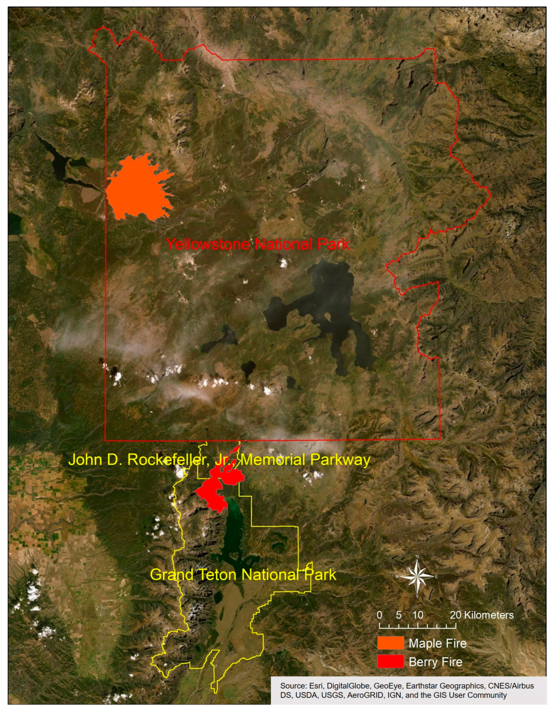
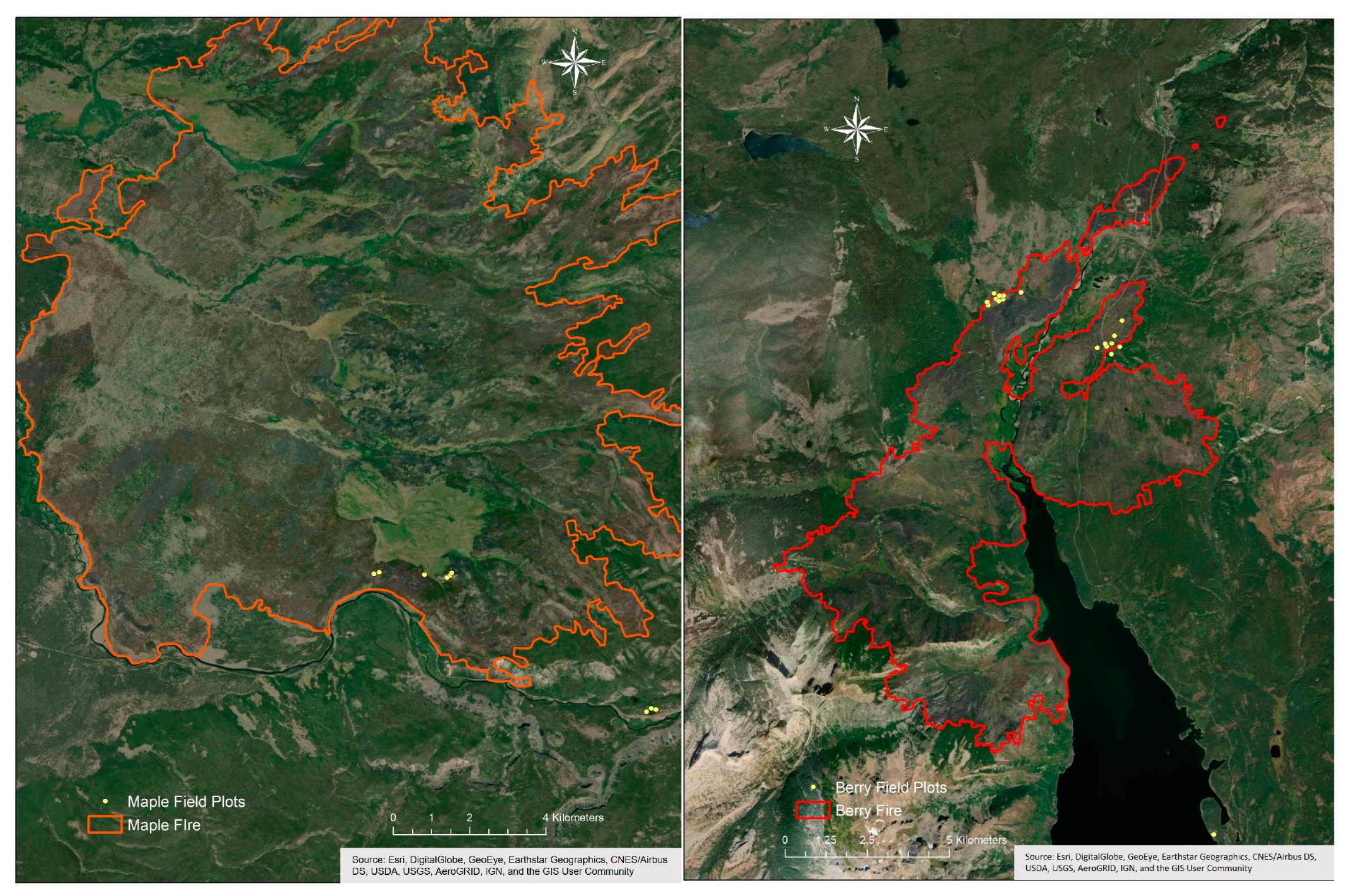
2.1. Study Area
2.2. Field Data
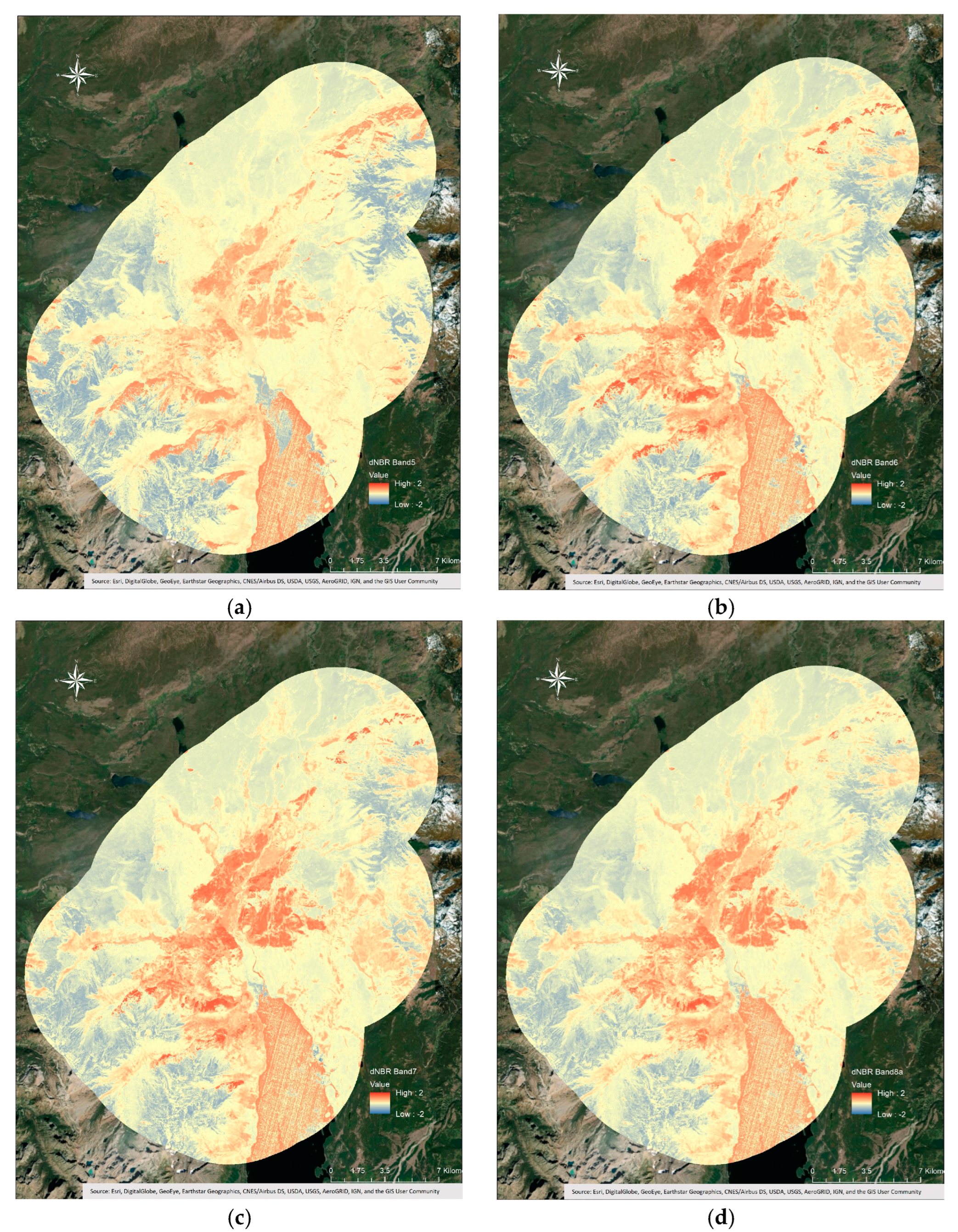
2.3. Image Prepossessing and Index Generation
2.4. Analysis
3. Results
3.1. Descriptive Statistics for Spectral Indices
3.2. Correlation Results
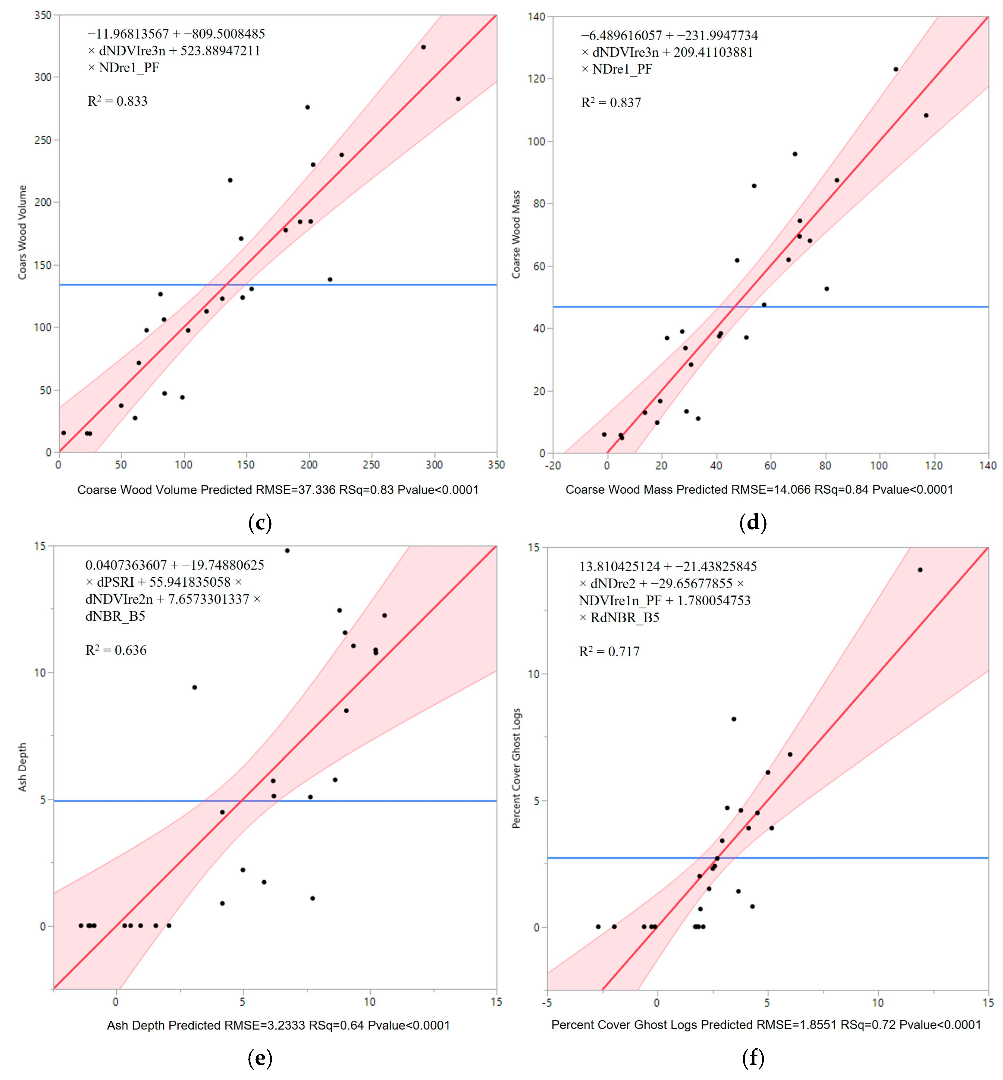
3.3. Regression Results
4. Discussion
4.1. Correlations between Spectral Indices and Field Measurements
4.2. Spectral Indices’ Ability to Estimate Field Measurements
4.3. Performance of Red-Edge Bands and Indices
4.4. Sources of Uncertainty
5. Conclusions
Author Contributions
Funding
Data Availability Statement
Acknowledgments
Conflicts of Interest
References
- Keeley, J.E. Fire Intensity, Fire Severity and Burn Severity: A Brief Review and Suggested Usage. Int. J. Wildland Fire 2009, 18, 116–126. [Google Scholar] [CrossRef]
- Robichaud, P.R.; Lewis, S.A.; Laes, D.Y.M.; Hudak, A.T.; Kokaly, R.F.; Zamudio, J.A. Postfire Soil Burn Severity Mapping with Hyperspectral Image Unmixing. Remote Sens. Environ. 2007, 108, 467–480. [Google Scholar] [CrossRef]
- Morgan, P.; Keane, R.E.; Dillon, G.K.; Jain, T.B.; Hudak, A.T.; Karau, E.C.; Sikkink, P.G.; Holden, Z.A.; Strand, E.K.; Morgan, P.; et al. Challenges of Assessing Fire and Burn Severity Using Field Measures, Remote Sensing and Modelling. Int. J. Wildland Fire 2014, 23, 1045–1060. [Google Scholar] [CrossRef]
- Key, C.H.; Benson, N.C. Landscape Assessment (LA). In FIREMON: Fire Effects Monitoring and Inventory System; Lutes, D.C., Keane, R.E., Caratti, J.F., Key, C.H., Benson, N.C., Sutherland, S., Gangi, L.J., Eds.; Gen. Tech. Rep. RMRS-GTR-164-CD; U.S. Department of Agriculture, Forest Service, Rocky Mountain Research Station: Fort Collins, CO, USA, 2006; p. LA-1-55. [Google Scholar]
- Epting, J.; Verbyla, D.; Sorbel, B. Evaluation of Remotely Sensed Indices for Assessing Burn Severity in Interior Alaska Using Landsat TM and ETM+. Remote Sens. Environ. 2005, 96, 328–339. [Google Scholar] [CrossRef]
- Roy, D.P.; Boschetti, L.; Trigg, S.N. Remote Sensing of Fire Severity: Assessing the Performance of the Normalized Burn Ratio. IEEE Geosci. Remote Sens. Lett. 2006, 3, 112–116. [Google Scholar] [CrossRef]
- Miller, J.D.; Thode, A.E. Quantifying Burn Severity in a Heterogeneous Landscape with a Relative Version of the Delta Normalized Burn Ratio (DNBR). Remote Sens. Environ. 2007, 109, 66–80. [Google Scholar] [CrossRef]
- Parks, S.A.; Dillon, G.K.; Miller, C. A New Metric for Quantifying Burn Severity: The Relativized Burn Ratio. Remote Sens. 2014, 6, 1827–1844. [Google Scholar] [CrossRef]
- Earth Observation of Wildland Fires in Mediterranean Ecosystems; Chuvieco, E., Ed.; Springer: Berlin/Heidelberg, Germany, 2009; ISBN 978-3-642-01753-7. [Google Scholar]
- Harris, S.; Veraverbeke, S.; Hook, S. Evaluating Spectral Indices for Assessing Fire Severity in Chaparral Ecosystems (Southern California) Using MODIS/ASTER (MASTER) Airborne Simulator Data. Remote Sens. 2011, 3, 2403–2419. [Google Scholar] [CrossRef]
- Quintano, C.; Fernández-Manso, A.; Calvo, L.; Marcos, E.; Valbuena, L. Land Surface Temperature as PotentialIndicator of Burn Severity in Forest Mediterranean Ecosystems. Int. J. Appl. Earth Obs. Geoinf. 2015, 36, 1–12. [Google Scholar] [CrossRef]
- Gitas, I.; Mitri, G.; Veraverbeke, S.; Polychronaki, A. Advances in Remote Sensing of Post-Fire Vegetation Recovery—A Review. In Remote Sensing of Biomass—Principles and Applications; Fatoyinbo, L., Ed.; InTechOpen: London, UK, 2012; ISBN 978-953-51-0313-4. [Google Scholar]
- Veraverbeke, S.; Hook, S.J. Evaluating Spectral Indices and Spectral Mixture Analysis for Assessing Fire Severity, Combustion Completeness and Carbon Emissions. Int. J. Wildland Fire 2013, 22, 707–720. [Google Scholar] [CrossRef]
- Fernández-Manso, A.; Fernández-Manso, O.; Quintano, C. SENTINEL-2A Red-Edge Spectral Indices Suitability for Discriminating Burn Severity. Int. J. Appl. Earth Obs. Geoinf. 2016, 50, 170–175. [Google Scholar] [CrossRef]
- Saberi, S.J. Quantifying Burn Severity in Forests of the Interior Pacific Northwest: From Field Measurements to Satellite Spectral Indices. M.S. Thesis, University of Washington, Seattle, Washington, USA, 2019. [Google Scholar]
- Hudak, A.T.; Morgan, P.; Bobbitt, M.J.; Smith, A.M.S.; Lewis, S.A.; Lentile, L.B.; Robichaud, P.R.; Clark, J.T.; McKinley, R.A. The Relationship of Multispectral Satellite Imagery to Immediate Fire Effects. Fire Ecol. 2007, 3, 64–90. [Google Scholar] [CrossRef]
- Turner, M.G.; Braziunas, K.H.; Hansen, W.D.; Harvey, B.J. Plot-level field data and model simulation results, archived to accompany Turner et al. manuscript; reports data from summer 2017 sampling of short-interval fires that burned during summer 2016 in Greater Yellowstone. ver 2. Environmental Data Initiative. 2019. Available online: https://portal.edirepository.org/nis/mapbrowse?packageid=edi.361.2 (accessed on 12 May 2020).
- Turner, M.G.; Braziunas, K.H.; Hansen, W.D.; Harvey, B.J. Short-Interval Severe Fire Erodes the Resilience of Subalpine Lodgepole Pine Forests. Proc. Natl. Acad. Sci. USA 2019, 116, 11319–11328. [Google Scholar] [CrossRef]
- Gitelson, A.; Merzlyak, M.N. Spectral Reflectance Changes Associated with Autumn Senescence of Aesculus Hippocastanum L. and Acer Platanoides L. Leaves. Spectral Features and Relation to Chlorophyll Estimation. J. Plant Physiol. 1994, 143, 286–292. [Google Scholar] [CrossRef]
- Haaland, D.M.; Thomas, E.V. Partial Least-Squares Methods for Spectral Analyses. 2. Application to Simulated and Glass Spectral Data. Anal. Chem. 1988, 60, 1202–1208. [Google Scholar] [CrossRef]
- Navarro, G.; Caballero, I.; Silva, G.; Parra, P.-C.; Vázquez, Á.; Caldeira, R. Evaluation of Forest Fire on Madeira Island Using Sentinel-2A MSI Imagery. Int. J. Appl. Earth Obs. Geoinf. 2017, 58, 97–106. [Google Scholar] [CrossRef]
- Verbyla, D.; Lord, R. Estimating Post-fire Organic Soil Depth in the Alaskan Boreal Forest Using the Normalized Burn Ratio. Int. J. Remote Sens. 2008, 29, 3845–3853. [Google Scholar] [CrossRef]
- Lentile, L.B.; Smith, A.M.S.; Hudak, A.T.; Morgan, P.; Bobbitt, M.J.; Lewis, S.A.; Robichaud, P.R.; Lentile, L.B.; Smith, A.M.S.; Hudak, A.T.; et al. Remote Sensing for Prediction of 1-Year Post-Fire Ecosystem Condition. Int. J. Wildland Fire 2009, 18, 594–608. [Google Scholar] [CrossRef]
- García-Llamas, P.; Suárez-Seoane, S.; Fernández-Guisuraga, J.M.; Fernández-García, V.; Fernández-Manso, A.; Quintano, C.; Taboada, A.; Marcos, E.; Calvo, L. Evaluation and Comparison of Landsat 8, Sentinel-2 and Deimos-1 Remote Sensing Indices for Assessing Burn Severity in Mediterranean Fire-Prone Ecosystems. Int. J. Appl. Earth Obs. Geoinf. 2019, 80, 137–144. [Google Scholar] [CrossRef]
- Howe, A.A.; Parks, S.A.; Harvey, B.J.; Saberi, S.J.; Lutz, J.A.; Yocom, L.L. Comparing Sentinel-2 and Landsat 8 for Burn Severity Mapping in Western North America. Remote Sens. 2022, 14, 5249. [Google Scholar] [CrossRef]
- Chuvieco, E.; Riaño, D.; Danson, F.M.; Martin, P. Use of a Radiative Transfer Model to Simulate the Postfire Spectral Response to Burn Severity. J. Geophys. Res. Biogeosci. 2006, 111, G04S09. [Google Scholar] [CrossRef]
- Korets, M.A.; Ryzhkova, V.A.; Danilova, I.V.; Sukhinin, A.I.; Bartalev, S.A. Forest Disturbance Assessment UsingSatellite Data of Moderate and Low Resolution. In Environmental Change in Siberia: Earth Observation, Field Studies and Modelling; Balzter, H., Ed.; Advances in Global Change Research; Springer: Dordrecht, The Netherlands, 2010; pp. 3–19. ISBN 978-90-481-8641-9. [Google Scholar]


| Field Measurement | Definition | Unit of Measurement |
|---|---|---|
| Post-fire Dead PICO Density | For plots that reburned, the density of fire-killed lodgepole pine trees | Number per hectare |
| Post-Fire Dead PICO Stumps | For plots that reburned, the density of stumps remaining for which the pre-fire lodgepole pine tree was completely combusted | Number per hectare |
| Mean Basal Diameter | The mean value from 25 measured live trees (on plots that did not reburn) or fire-killed trees or stumps (in reburned plots) | Centimeters |
| Cone Density on Dead Post-fire Trees | In plots that reburned, the remaining identifiable cones on fire-killed lodgepole pine trees | Number per hectare |
| Coarse Wood Percent Cover | Percent of surface covered by downed coarse wood, estimated via line intercept | Cubic meters per hectare |
| Coarse Wood Volume | Volume of coarse wood estimated via Brown’s planar intercept transects; in reburned plots, this is the volume of wood remaining after the short-interval fire | Megagrams per hectare |
| Coarse Wood Mass | Mass of coarse wood estimated via Brown’s planar intercept transects; in reburned plots, this is the volume of wood remaining after the short-interval fire | Millimeters |
| Ash Depth | Where recent ash was visible, depth on soil surface | Millimeters |
| Char Depth | If soil showed evidence of charring, depth from surface to which soil charring was evident | Millimeters |
| Percent Cover of Ghost Logs | On reburned plots, areas of soil surface covered by log shadows where downed coarse wood had been combusted completely | Dimensionless |
| Initial Regeneration of Post-fire PICO Density | Density of first-year seedlings of lodgepole pine | Number per hectare |
| Initial Regeneration of Post-fire Aspen Density | Density of aspen stumps that resprouted from surviving roots; if multiple leaders came from the same stump, it was scored as one | Number per hectare |
| Spectral Indices | Column 2 | Equation |
|---|---|---|
| NBR | Normalized Burn Ratio | |
| NDVI | Normalized Difference Vegetation Index | |
| GNDVI | Green Normalized Difference Vegetation Index | |
| NDVIre1n | Normalized Difference Vegetation Index red-edge 1 narrow | |
| NDVIre2n | Normalized Difference Vegetation Index red-edge 2 narrow | |
| NDVIre3n | Normalized Difference Vegetation Index red-edge 3 narrow | |
| PSRI | Plant Senescence Reflectance Index | |
| Clre | Chlorophyll Index re-edge | |
| Ndre1 | Normalized Difference re-edge 1 | |
| Ndre2 | Normalized Difference red-edge 2 | |
| MSRren | Modified Simple Ratio red-edge narrow |
| Index | Min | Max | Mean | Standard Deviation |
|---|---|---|---|---|
| Post-fire Normalized Red-edge Indices | ||||
| NDre1_PF | −0.994 | 0.997 | 0.130 | 0.222 |
| NDre2_PF | −0.994 | 0.998 | 0.154 | 0.244 |
| NDVIre1n_PF | −0.996 | 0.998 | 0.178 | 0.264 |
| NDVIre2n_PF | −0.986 | 0.993 | 0.060 | 0.109 |
| NDVIre3n_PF | −0.987 | 0.992 | 0.031 | 0.078 |
| Difference Normalized Red-edge Indices | ||||
| dNDre1 | −1.202 | 1.805 | 0.025 | 0.152 |
| dNDre2 | −1.719 | 1.946 | 0.026 | 0.151 |
| dNDVIre1n | −1.857 | 1.892 | 0.017 | 0.145 |
| dNDVIre2n | −1.747 | 1.787 | −0.011 | 0.094 |
| dNDVIre3n | −1.886 | 1.798 | −0.013 | 0.078 |
| Difference Normalized Burn Ratios | ||||
| dNBR_B8a | −1.749 | 1.637 | 0.010 | 0.423 |
| dNBR_B5 | −1.798 | 1.666 | −0.036 | 0.436 |
| dNBR_B6 | −1.769 | 1.627 | 0.026 | 0.479 |
| dNBR_B7 | −1.736 | 1.693 | 0.030 | 0.460 |
| Other Burn Ratios | ||||
| RdNBR_B8a | −73.309 | 32.330 | −0.133 | 1.612 |
| RdNBR_B5 | −84.548 | 42.966 | −0.318 | 2.002 |
| RdNBR_B6 | −68.660 | 48.944 | −0.214 | 1.937 |
| RdNBR_B7 | −75.090 | 28.094 | −0.148 | 1.765 |
| RBR_B8a | −70.076 | 0.994 | −0.014 | 0.442 |
| RBR_B5 | −198.320 | 0.996 | −0.073 | 0.609 |
| RBR_B6 | −161.290 | 0.997 | −0.021 | 0.657 |
| RBR_B7 | −159.930 | 0.997 | −0.007 | 0.534 |
| Other Indices | ||||
| GNDVI_PF | −0.997 | 0.999 | 0.270 | 0.436 |
| PSRI_PF | −280.000 | 80.000 | −2.107 | 17.112 |
| MSRren_PF | −0.997 | 28.284 | 0.466 | 1.194 |
| CLre_PF | −3836.000 | 3662.000 | 217.252 | 365.007 |
| dGNDVI | −1.627 | 1.624 | 0.012 | 0.205 |
| dPSRI | −295.300 | 279.860 | 1.944 | 17.172 |
| dMSRren | −27.486 | 15.185 | −0.081 | 1.048 |
| dCLre | −2740.000 | 4979.000 | 297.265 | 523.168 |
| Index | Min | Max | Mean | Standard Deviation |
|---|---|---|---|---|
| Post-fire Normalized Red-edge Indices | ||||
| NDre1_PF | −0.829 | 0.947 | 0.168 | 0.138 |
| NDre2_PF | −0.991 | 0.967 | 0.204 | 0.155 |
| NDVIre1n_PF | −0.990 | 0.941 | 0.238 | 0.165 |
| NDVIre2n_PF | −0.981 | 0.882 | 0.077 | 0.047 |
| NDVIre3n_PF | −0.974 | 0.994 | 0.037 | 0.027 |
| Difference Normalized Red-edge Indices | ||||
| dNDre1 | −0.912 | 0.708 | 0.049 | 0.123 |
| dNDre2 | −0.867 | 0.735 | 0.057 | 0.128 |
| dNDVIre1n | −0.828 | 0.893 | 0.059 | 0.117 |
| dNDVIre2n | −1.172 | 0.997 | 0.015 | 0.022 |
| dNDVIre3n | −1.022 | 0.762 | 0.005 | 0.020 |
| Difference Normalized Burn Ratios | ||||
| dNBR_B8a | −0.888 | 1.229 | 0.159 | 0.294 |
| dNBR_B5 | −1.207 | 0.938 | 0.072 | 0.181 |
| dNBR_B6 | −1.028 | 1.260 | 0.140 | 0.301 |
| dNBR_B7 | −0.969 | 1.268 | 0.154 | 0.306 |
| Other Burn Ratios | ||||
| RdNBR_B8a | −59.367 | 18.309 | 0.248 | 0.652 |
| RdNBR_B5 | −15.804 | 23.850 | 0.352 | 1.120 |
| RdNBR_B6 | −45.937 | 26.669 | 0.275 | 0.994 |
| RdNBR_B7 | −56.675 | 23.814 | 0.257 | 0.827 |
| RBR_B8a | −7.268 | 0.985 | 0.114 | 0.214 |
| RBR_B5 | −1.747 | 0.983 | 0.076 | 0.196 |
| RBR_B6 | −69.379 | 0.852 | 0.106 | 0.259 |
| RBR_B7 | −53.673 | 0.989 | 0.112 | 0.243 |
| Other Indices | ||||
| GNDVI_PF | −0.985 | 0.995 | 0.409 | 0.250 |
| PSRI_PF | −9.818 | 1.238 | 0.053 | 0.087 |
| MSRren_PF | −0.993 | 5.488 | 0.423 | 0.319 |
| CLre_PF | −1447.000 | 4516.000 | 556.645 | 540.477 |
| dGNDVI | −0.717 | 1.349 | 0.058 | 0.113 |
| dPSRI | −1.211 | 13.981 | −0.014 | 0.097 |
| dMSRren | −5.318 | 1.423 | 0.130 | 0.262 |
| dCLre | −1447.000 | 13.981 | −0.014 | 0.097 |
| Index | Post-fire Dead PICO Density | Post-fire Dead PICO Stumps | Mean Basal Diameter | Post-fire Cone Density | Coarse Wood Percent | Coarse Wood Volume | Coarse Wood Mass | Ash Depth | Char Depth | Percent Cover of Ghost Logs | Initial Regen | Initial Regen Aspen |
|---|---|---|---|---|---|---|---|---|---|---|---|---|
| PICO | ||||||||||||
| dCLre_Avg | 0.294 | 0.358 | −0.167 | 0.443 | −0.669 | −0.551 | −0.617 | 0.674 | 0.227 | 0.518 | 0.274 | 0.346 |
| dPSRI_Avg | −0.170 | −0.078 | 0.001 | −0.295 | 0.529 | 0.367 | 0.438 | −0.515 | −0.440 | −0.387 | −0.038 | −0.328 |
| MSRren_AVG | 0.283 | 0.636 | −0.417 | 0.345 | −0.636 | −0.754 | −0.742 | 0.572 | −0.195 | 0.491 | 0.484 | 0.094 |
| NDre1_Avg | 0.352 | 0.565 | −0.354 | 0.462 | −0.756 | −0.765 | −0.798 | 0.696 | 0.088 | 0.581 | 0.414 | 0.190 |
| NDre2_AVG | 0.346 | 0.658 | −0.428 | 0.418 | −0.752 | −0.793 | −0.811 | 0.697 | −0.021 | 0.580 | 0.450 | 0.139 |
| NDVIre1n_A | 0.291 | 0.726 | −0.481 | 0.291 | −0.657 | −0.777 | −0.763 | 0.626 | −0.160 | 0.552 | 0.460 | 0.065 |
| NDVIre2n_A | −0.139 | 0.228 | −0.183 | −0.326 | 0.243 | 0.037 | 0.126 | −0.194 | −0.477 | −0.111 | 0.070 | −0.240 |
| NDVIre3n_A | −0.040 | 0.344 | −0.537 | −0.172 | −0.057 | −0.430 | −0.354 | 0.107 | −0.315 | 0.201 | 0.131 | −0.005 |
| CLre_PF_Avg | −0.316 | −0.347 | 0.204 | −0.379 | 0.671 | 0.587 | 0.658 | −0.673 | −0.281 | −0.587 | −0.260 | −0.286 |
| PSRI_PF_AVG | 0.142 | 0.018 | 0.034 | 0.263 | −0.499 | −0.337 | −0.413 | 0.469 | 0.472 | 0.371 | 0.001 | 0.318 |
| MSR_PF_AVG | −0.145 | −0.623 | 0.524 | −0.026 | 0.650 | 0.808 | 0.776 | −0.485 | 0.185 | −0.580 | −0.331 | −0.120 |
| NDre1_PF_AVG | −0.258 | −0.557 | 0.431 | −0.257 | 0.821 | 0.855 | 0.883 | −0.668 | −0.139 | −0.688 | −0.312 | −0.212 |
| NDre2_PF_AVG | −0.235 | −0.658 | 0.522 | −0.174 | 0.805 | 0.879 | 0.886 | −0.649 | 0.001 | −0.686 | −0.337 | −0.162 |
| NDVIr1_PF_A | −0.167 | −0.707 | 0.570 | −0.022 | 0.671 | 0.826 | 0.798 | −0.548 | 0.153 | −0.630 | −0.330 | −0.085 |
| NDVIr2_PF_A | 0.133 | −0.280 | 0.259 | 0.367 | −0.172 | 0.035 | −0.059 | 0.153 | 0.485 | 0.038 | −0.062 | 0.181 |
| NDVIr3_PF_AVG | 0.168 | −0.162 | 0.147 | 0.375 | −0.260 | −0.042 | −0.137 | 0.230 | 0.431 | 0.089 | −0.020 | 0.161 |
| dNBR_B5_AVG | 0.415 | 0.326 | −0.277 | 0.551 | −0.612 | −0.569 | −0.641 | 0.667 | 0.290 | 0.443 | 0.372 | 0.195 |
| dNBR_B6_AVG | 0.418 | 0.358 | −0.299 | 0.539 | −0.626 | −0.589 | −0.656 | 0.683 | 0.238 | 0.477 | 0.359 | 0.230 |
| dNBR_B7_AVG | 0.412 | 0.385 | −0.293 | 0.549 | −0.641 | −0.600 | −0.667 | 0.687 | 0.266 | 0.484 | 0.380 | 0.197 |
| dNBR_8a_AVG | 0.417 | 0.414 | −0.319 | 0.547 | −0.644 | −0.619 | −0.682 | 0.703 | 0.257 | 0.499 | 0.397 | 0.190 |
| RBR_B5_AVG | 0.388 | 0.272 | −0.249 | 0.519 | −0.610 | −0.552 | −0.626 | 0.650 | 0.333 | 0.463 | 0.325 | 0.346 |
| RBR_B6_AVG | 0.382 | 0.334 | −0.278 | 0.501 | −0.658 | −0.603 | −0.671 | 0.678 | 0.314 | 0.520 | 0.274 | −0.328 |
| RBR_B7_AVG | 0.387 | 0.356 | −0.294 | 0.501 | −0.660 | −0.608 | −0.675 | 0.688 | 0.306 | 0.518 | −0.038 | 0.094 |
| RBR_8a_AVG | 0.396 | 0.390 | −0.322 | 0.503 | −0.663 | −0.630 | −0.693 | 0.706 | 0.293 | −0.387 | 0.484 | 0.190 |
| RdNBR_B5_AVG | 0.383 | 0.326 | −0.180 | 0.520 | −0.425 | −0.414 | −0.479 | 0.468 | 0.227 | 0.491 | 0.414 | 0.139 |
| RdNBR_B6_AVG | 0.208 | 0.172 | −0.253 | 0.273 | −0.615 | −0.554 | −0.614 | 0.674 | −0.440 | 0.581 | 0.450 | 0.065 |
| RdNBR_B7_AVG | 0.228 | 0.205 | −0.250 | 0.296 | −0.673 | −0.584 | −0.617 | −0.515 | −0.195 | 0.580 | 0.460 | −0.240 |
| RdNBR_8a_AVG | 0.353 | 0.349 | −0.325 | 0.441 | −0.687 | −0.551 | 0.438 | 0.572 | 0.088 | 0.552 | 0.070 | −0.005 |
| GNDVI_AVG | 0.237 | 0.709 | −0.541 | 0.124 | −0.669 | 0.367 | −0.742 | 0.696 | −0.021 | −0.111 | 0.131 | −0.286 |
| NDVI_AVG | 0.357 | 0.705 | −0.479 | 0.443 | 0.529 | −0.754 | −0.798 | 0.697 | −0.160 | 0.201 | −0.260 | 0.318 |
| GNDVI_PF_AVG | −0.131 | −0.673 | −0.167 | −0.295 | −0.636 | −0.765 | −0.811 | 0.626 | −0.477 | −0.587 | 0.001 | −0.120 |
| Field Measurement | Model Variables | R2 | RMSE | PRESS R2 | PRESS RMSE |
|---|---|---|---|---|---|
| Post-fire Dead PICO Density | dNBR_B6 | 0.174 | 16,859.88 | 0.066 | 17,255.543 |
| Post-fire Dead PICO Density | None | N/A | N/A | N/A | N/A |
| Post-fire Dead PICO Density | None | N/A | N/A | N/A | N/A |
| Post-fire Dead PICO Stumps | dNDVIre1n | 0.527 | 21,687.91 | 0.383 | 23,854.682 |
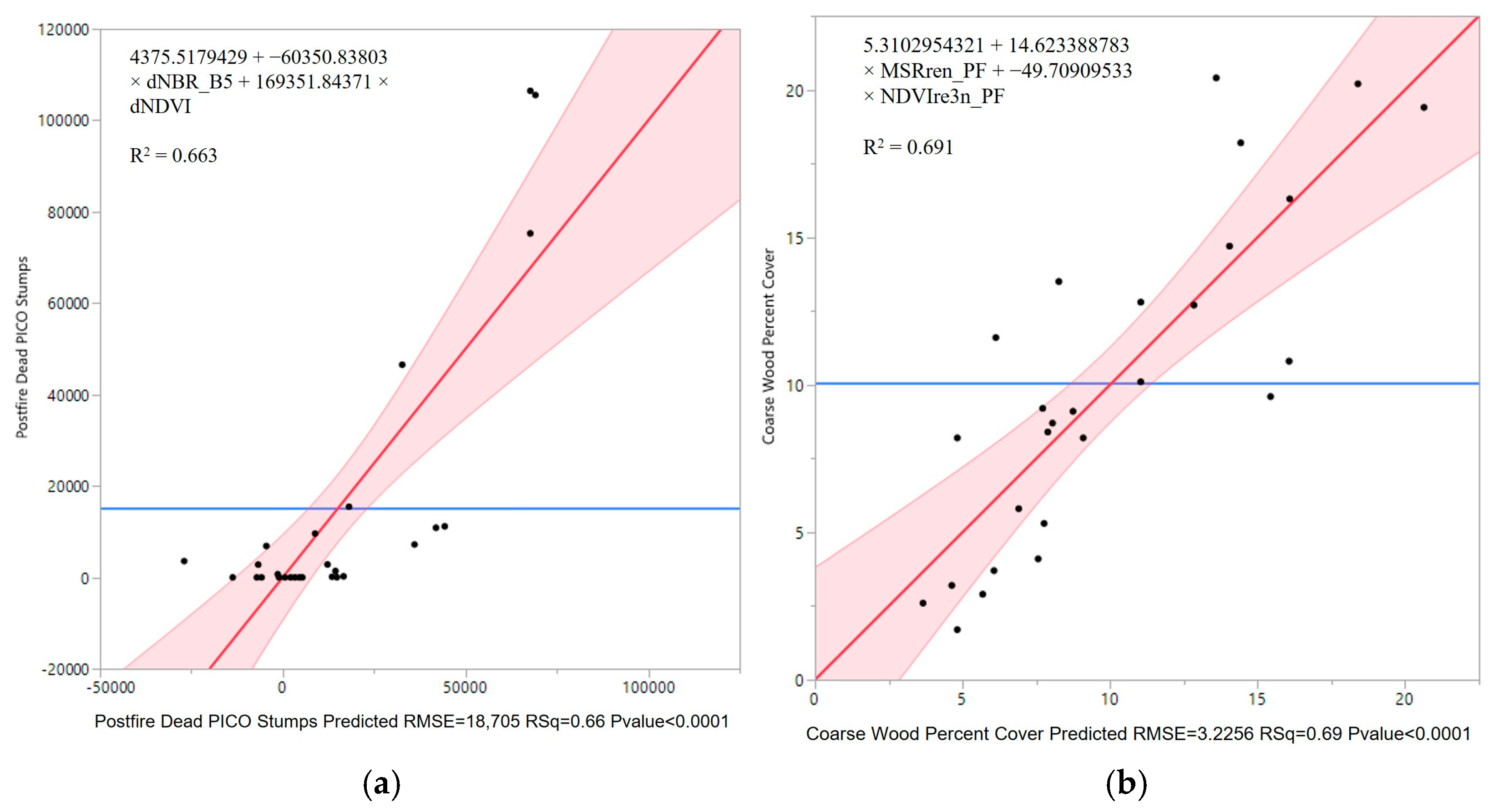
| Post-fire Dead PICO Stumps | dNBR_B5, dNDVI | 0.663 | 18,705.19 | 0.502 | 21,414.479 |
| Post-fire Dead PICO Stumps | None | N/A | N/A | N/A | N/A |
| Mean Basal Diameter | GNDVI_PF | 0.349 | 2.542 | 0.248 | 2.629 |
| Mean Basal Diameter | dNDVIre3n, NDre2_PF | 0.440 | 2.406 | 0.2853 | 2.562 |
| Mean Basal Diameter | None | N/A | N/A | N/A | N/A |
| Cone Density on Dead Post-fire Trees | dNBR_B5 | 0.304 | 75,553.4 | 0.184 | 78,703.305 |
| Cone Density on Dead Post-fire Trees | dNDre2, NDVIre1n_PF | 0.419 | 70,417.16 | 0.2411 | 75,900.966 |
| Cone Density on Dead Post-fire Trees | dPSRI, dMSRren, NDVIre2n_PF | 0.571 | 61,865.44 | 0.333 | 71,184.947 |
| Coarse Wood Percent Cover | NDre1_PF | 0.674 | 3.244 | 0.620 | 3.370 |
| Coarse Wood Percent Cover | MSRren_PF, dNDVIre3n | 0.691 | 3.226 | 0.627 | 3.341 |
| Coarse Wood Percent Cover | None | N/A | N/A | N/A | N/A |
| Coarse Wood Volume | NDre2_PF | 0.773 | 42.735 | 0.7403 | 43.944 |
| Coarse Wood Volume | dNDVIre3n, NDre1_PF | 0.833 | 37.336 | 0.782 | 40.229 |
| Coarse Wood Volume | None | N/A | N/A | N/A | N/A |
| Coarse Wood Mass | NDre2_PF | 0.784 | 15.878 | 0.753 | 16.367 |
| Coarse Wood Mass | dNDVIre3n, NDre1_PF | 0.838 | 14.066 | 0.787 | 15.175 |
| Coarse Wood Mass | dNDVIre3n, NDre2_PF, NDVIre2n_PF | 0.842 | 14.157 | 0.770 | 15.776 |
| Ash Depth | dNDVI | 0.548 | 3.455 | 0.493 | 3.520 |
| Ash Depth | dCLre, dNDVIre3n | 0.581 | 3.396 | 0.486 | 3.543 |
| Ash Depth | dPSRI, dNDVIre2n, dNBR_B5 | 0.636 | 3.233 | 0.392 | 3.853 |
| Char Depth | NDVIre2n_PF | 0.235 | 0.177 | −0.008 | 0.195 |
| Char Depth | dNDre2, RBR_B8a | 0.328 | 0.169 | 0.148 | 0.179 |
| Char Depth | None | N/A | N/A | N/A | N/A |
| Percent Cover of Ghost Logs | NDre1_PF | 0.473 | 2.430 | 0.361 | 2.574 |
| Percent Cover of Ghost Logs | NDVIre1n_PF, RdNBR_B5 | 0.587 | 2.194 | 0.421 | 2.450 |
| Percent Cover of Ghost Logs | dNDre2, NDVIre1n_PF, RdNBR_B5 | 0.717 | 1.855 | 0.574 | 2.100 |
| Initial Regeneration of Post-fire PICO Density | dMSRren | 0.234 | 8440.969 | 0.030 | 9140.458 |
| Initial Regeneration of Post-fire PICO Density | RBR_B6, PSRI_PF | 0.328 | 8071.69 | 0.078 | 8915.812 |
| Initial Regeneration of Post-fire PICO Density | None | N/A | N/A | N/A | N/A |
| Initial Regeneration of Post-fire Aspen Density | None | N/A | N/A | N/A | N/A |
| Initial Regeneration of Post-fire Aspen Density | MSRren_PF, GNDVI_PF | 0.249 | 81.299 | 0.037 | 86.791 |
| Initial Regeneration of Post-fire Aspen Density | dCLre, dNDVIer3n, dNDVI | 0.448 | 71.177 | 0.224 | 77.933 |
Disclaimer/Publisher’s Note: The statements, opinions and data contained in all publications are solely those of the individual author(s) and contributor(s) and not of MDPI and/or the editor(s). MDPI and/or the editor(s) disclaim responsibility for any injury to people or property resulting from any ideas, methods, instructions or products referred to in the content. |
© 2023 by the authors. Licensee MDPI, Basel, Switzerland. This article is an open access article distributed under the terms and conditions of the Creative Commons Attribution (CC BY) license (https://creativecommons.org/licenses/by/4.0/).
Share and Cite
Szpakowski, D.M.; Jensen, J.L.R.; Chow, T.E.; Butler, D.R. Assessing the Use of Burn Ratios and Red-Edge Spectral Indices for Detecting Fire Effects in the Greater Yellowstone Ecosystem. Forests 2023, 14, 1508. https://doi.org/10.3390/f14071508
Szpakowski DM, Jensen JLR, Chow TE, Butler DR. Assessing the Use of Burn Ratios and Red-Edge Spectral Indices for Detecting Fire Effects in the Greater Yellowstone Ecosystem. Forests. 2023; 14(7):1508. https://doi.org/10.3390/f14071508
Chicago/Turabian StyleSzpakowski, David M., Jennifer L. R. Jensen, T. Edwin Chow, and David R. Butler. 2023. "Assessing the Use of Burn Ratios and Red-Edge Spectral Indices for Detecting Fire Effects in the Greater Yellowstone Ecosystem" Forests 14, no. 7: 1508. https://doi.org/10.3390/f14071508
APA StyleSzpakowski, D. M., Jensen, J. L. R., Chow, T. E., & Butler, D. R. (2023). Assessing the Use of Burn Ratios and Red-Edge Spectral Indices for Detecting Fire Effects in the Greater Yellowstone Ecosystem. Forests, 14(7), 1508. https://doi.org/10.3390/f14071508