Article

Aboveground Carbon Stock in a Bottomland Hardwood Forest in the Southeastern United States

by
Jared R. Streeter
,
Joydeep Bhattacharjee
* and
Bibek Kandel
Plant Ecology Lab, Biology Program, University of Louisiana Monroe, 700 University Avenue, Monroe, LA 71209, USA
*
Author to whom correspondence should be addressed.
Deceased author.
Forests 2023, 14(5), 974; https://doi.org/10.3390/f14050974
Submission received: 20 March 2023 / Revised: 24 April 2023 / Accepted: 2 May 2023 / Published: 9 May 2023
(This article belongs to the Section Forest Ecology and Management)

Abstract

:
Bottomland Hardwood Forests (BHFs) are commonly acknowledged worldwide for their vast carbon sequestration potential and carbon storage capacity. However, the paucity of forest carbon stock data from BHFs along the Lower Mississippi Alluvial Valley (LMAV) in Northeast Louisiana is an existing knowledge gap in understanding the carbon sequestration and storage dynamics across the region. This study was carried out in the Russell Sage Wildlife Management Area (RSWMA) in Northeast Louisiana using a protocol modified from the Terrestrial Carbon Observations Protocol for Vegetation Sampling. Comprehensive analyses of carbon stocks in trees, woody shrubs and seedlings, herbaceous vegetation, downed woody debris, leaf litter, and soil were carried out to quantify the carbon stored in each ecosystem component. Trees accounted for a carbon stock of 132.4 Mg C ha−1, approximately 99% of the total stock for the area. Woody shrubs and seedlings and leaf litter stored 0.4% (0.62 Mg C ha−1) and 0.3% (0.4 Mg C ha−1), respectively. Considering the sparse understory in a BHF, the carbon stored per hectare is comparable to other temperate forests in the conterminous United States. These findings highlight the importance of the BHF ecosystem in carbon storage and their overall role in regional and global ecosystem management in light of climate change.

1. Introduction

Forest Carbon Stocks

Evidence continues to mount in support of climate change due to a significant increase in carbon dioxide concentrations in the atmosphere [1,2,3,4]. Forests around the world are regarded as effective natural means of vast carbon sequestration potential and carbon storage capacity [5,6,7,8]. Bottomland Hardwood Forests (BHF), deciduous forested wetlands located in broad floodplain areas bordering large river systems such as the Mississippi, can help mitigate climate change due to their high carbon sequestration and subsequent storage potential [9,10]. However, land-use changes such as deforestation and agriculture continue to be the second most important source of CO2 emissions, exacerbating the climate impacts [11,12,13,14]. Reducing the occurrence of deforestation and preserving current forests alongside afforestation and reforestation efforts are both viable methods of mitigating climate change [15,16,17,18].
There are recognized variations in carbon storage among forests [9,12]. Therefore, it is important to determine the carbon stocks of individual forest types when possible. Various methods exist for estimating the aboveground biomass (AGB) and carbon stocks of vegetation, such as the use of species-specific allometric regression models [19,20,21], recent advances in remote sensing, and LIDAR [22,23,24]. Rapid assessments of AGB and carbon stocks for forests are often based on allometric regression models [25,26,27,28].
Forest ecosystems in the United States contain approximately 57.8 billion tons, around 4% of the total carbon stored in the world’s forests [19]. Previous regional studies based on statistical samples designed to represent a broad range of forest conditions report that forests in this region store on average 131 Mg C ha−1; however, these studies are at a regional scale, e.g., the forest in our study site has been clubbed with forests from West Texas to East Tennessee, which in itself encompasses a wide diversity of forest types [19]. While such studies are important, management recommendations and conservation strategies are often developed and implemented at local scales. Thus, a species-specific dedicated carbon assessment, representative of this ecosystem, is crucial for strategic management and informed decision making for this ecosystem. We believe that the information derived will subsequently contribute to heightening the conservation status of these forests since it has seen unprecedented loss (from 101,000 km2 in the LMAV in the 1920s to only 21,000 km2 in the 2010s) due to severe deforestation and agriculture [29,30,31,32]. This is the first study of the carbon stock in the region’s inland BHFs and, thus, fills in a data gap in the carbon budget from this region. Due to a lack of data from BHFs, the current state of regional and national carbon flux models remains incomplete. Therefore, it is timely to research the contribution of these unique forested ecosystems in maintaining the carbon balance and mitigating the impacts of climate change at regional and global scales. The need to better understand this ecosystem is further accentuated by the fact that the loss of these forests is associated with the loss of several ecosystem services, such as habitats for diverse flora and fauna, upland protection from flood and hurricanes, the storage of carbon, recreation, and the purification of water [33]. This study aims to quantify the standing AGB and carbon stock for major forest components such as trees, seedlings, and understory vegetation in a BHF.

2. Methods

2.1. Site Description

The study was carried out in the Russell Sage Wildlife Management Area (RSWMA, 32°27′25.02″ N and 91°58′27.78″ W), which comprises 8882 ha of land spanning three parishes within the Bayou Lafourche floodplain (Figure 1). A total of 4.48 ha area was sampled for this study. The RSWMA is located within the Bayou Lafourche floodplain and is subjected to annual winter to early spring flooding.
The physiographic forest positions of Southeastern United States forests are considered uplands, terraces, and floodplains [34]. The soil type is Perry Clay, fine-textured sediment that has low permeability and a moderate capacity to hold water [35]. The forest stand that was sampled for this study was estimated to be 70–90 years old (pers comm Larry Savage, Louisiana Department of Wildlife and Fisheries). In the Central and Southeastern United States, deciduous forested wetlands located in broad floodplain areas bordering large river systems such as within the LMAV are referred to as BHFs [36]. The BHFs in Northeast Louisiana are characterized by a unique flooding pattern in which much of the forest remains inundated during one half (December–May) of the year, resulting in alternating annual wet and dry seasons [37]. Typically, there are five recognized plant species associations of BHFs in the LMAV, Louisiana: overcup oak–water hickory, hackberry–American elm–green ash, black willow–cottonwood, live oak forest, and sweetgum–water oak [38]. However, the dominant association at the research site was oak–hickory, with several species under each genus. These highly productive and diverse ecosystems provide valuable ecosystem services and wildlife habitats [30].
The BHF of the RSWMA conforms best to the overcup oak–water hickory forest type [39]. Common tree species of the site include Nuttall oak (Quercus texana Buckley.), overcup oak (Quercus lyrate Walter), willow oak (Quercus phellos L.), water hickory (Carya aquatica (F. Michx.) Elliott), and sugarberry (Celtis laevigata Willd.). The understory vegetation for the site is dominated by Southern dewberry (Rubus trivialis Michx.), American buckwheat vine (Brunnichia ovata (Walter) Shinners), Alabama supplejack/rattan vine (Berchemia scandens (Hill) K. Koch), and poison ivy (Toxicodendron radicans (L.) Kuntze). The total leaf area index (LAI) was calculated to be 3.8 m2 for the site. AGB and carbon stock were determined using extensive field sampling and allometric equations. Additionally, forest components such as downed woody debris (DWD), soil, and leaf litter were also analyzed for their carbon stock. Other stores of carbon (belowground microorganisms, fungi, standing dead wood, etc.) were not sampled during this study but are understood to contribute to the overall carbon stock of the study area.

2.2. Data Collection

2.2.1. Vegetation Plot Layout

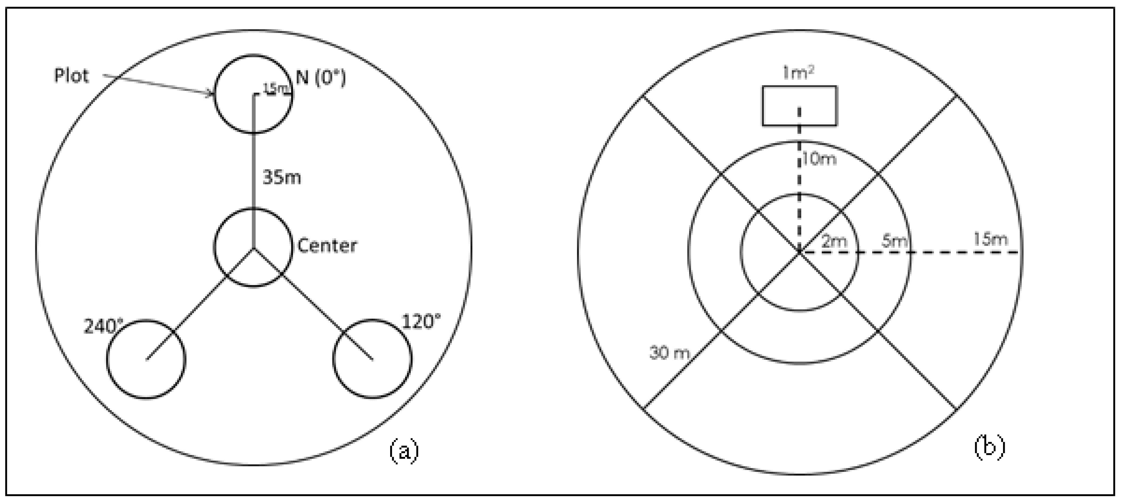
Sixteen 1-ha sites were established within the RSWMA using Google Earth imagery and a random number generator. Each site contained four plots consisting of one center plot and three other plots located at 0°, 120°, and 240° from the center (Figure 2a). The distance from each of these plots from the central plot was 35 m and each plot was 15 m in radius. The plots were established using a protocol modified from the Terrestrial Carbon Observations: Protocols for Vegetation Sampling and Data Submission (TCO) [40]. Within each plot, all trees with a diameter at breast height (DBH) ≥10 cm were counted, taxonomically identified, and measured. Next, the species name, height class (0.5–<1 m and 1–2 m), basal diameter, percent cover, and the number of individuals for all woody shrubs and seedlings were recorded in a nested 2 m radius plot (Figure 2b). In addition, estimation of vegetation biomass and visual obstruction measurements (VOM) were taken in a 1 m2 plot, 10 m north of each plot center. The coordinates for each plot center were recorded using a GPS unit, and a PVC pipe was used to mark the center. Species identification of all plants sampled was accomplished using a combination of field guides, the United States Department of Agriculture (USDA) Plants database, and the university herbarium at the University of Louisiana Monroe.

2.2.2. Trees

A total of 896 trees were sampled for this study. Species’ names, DBH, and height were recorded for each tree. If a tree had a bifurcated stem, it was treated as two separate trees when bifurcation occurred below the DBH (1.35 m).

2.2.3. Woody Shrubs and Seedlings

Basal diameter was measured to the nearest 0.01 mm using a pair of calipers. To develop a regression model for predicting AGB from basal diameter, woody shrubs and seedlings were randomly selected and harvested from areas of representative vegetation, outside of the permanent plots.

2.2.4. Understory Herbaceous Vegetation and Visual Obstruction Measurement

Vegetation cover in each 5 m radius plot was categorized as grasses/sedges/rushes, woody, herbaceous, forbs, moss/lichen, detritus, bare ground, and water. An ocular estimate of percent cover was measured for each of the categories. VOM was taken using a modified Robel pole. VOM for the plot was taken from each cardinal direction and averaged for the plot. Ground cover estimates were also taken for each of the aforementioned categories using a 1 m2 plot.
To estimate understory vegetation AGB, 10 sacrificial plots were used to develop a regression model of VOM and understory AGB. Ten additional 1 m2 sacrificial plots were located outside the permanent plots, ensuring that they contained representative vegetation of the study plot, and equations were developed for AGB estimates.

2.2.5. Downed Woody Debris

Downed woody debris (DWD) was measured in each plot along 15 m transects radiating from the center to the NE, SE, SW, and NW directions. Woody debris with a diameter ≥7.6 cm was categorized as coarse woody debris (CWD) and measured along the entire transect. Woody debris with a diameter of less than 7.6 cm was categorized as fine woody debris (FWD) and sampled along the entire transect. The total number of “hits” of FWD was tallied according to size classes (0.6–2.5 cm and 2.5–7.6 cm) and the diameter for each piece of CWD was recorded. All CWD diameter measurements and FWD hits were made at the point of intersection along transects. AGB estimations for DWD were conducted following protocols put forth by Law et al. (2008) [40].

2.2.6. Soil

Based on the Natural Resource Conservation Survey (NRCS) soil survey map of the area, the soil in the area was Perry Clay. Due to the expected homogeneity of soil across the area, soil cores were obtained from 16 plots using a soil probe. One sample was taken from each of the sites to obtain representative samples for the overall area. The depths of each sample and plot number were recorded and brought back to the lab for carbon content analysis.

2.2.7. Leaf Litter

The protocol for collecting leaf litter samples was adopted from methods put forth by Giese and Law [40,41]. Litter samples were collected from ten 1 m2 plots spread across the study area to determine the carbon content. Litter (detritus) for this study is defined according to the surface layer of the forest floor containing fresh/dry, dead, and partially decomposed plant tissue [40].

2.3. Estimation of Aboveground Biomass and Carbon Stocks

2.3.1. Trees

AGB for trees (DBH ≥ 10 cm) was estimated using allometric equations obtained from previous research [26,41,42,43] and the GlobAllomeTree database [44]. Based on the findings of previous literature, the carbon content for trees in the area was calculated as 50% of AGB [12,15,21,41,45,46]. Carbon stock was then summed for all trees in each plot and the results were scaled from kg C per plot to Mg C (103 kg) per hectare.

2.3.2. Woody Shrubs and Seedlings

Woody shrubs and seedlings harvested in the sacrificial plots were brought back to the lab and weighed to the nearest 0.01 g to obtain the wet weight. The samples were then dried at 60 °C for 4 days until a constant dry weight was reached. AGB was determined using a regression model developed from this study and carbon content was calculated based on the literature as 47% of AGB [12,46].

2.3.3. Understory Herbaceous Vegetation

Samples collected from the field were weighed and placed into a drying oven. Samples were dried at 60 °C for 3–4 days until a constant weight was reached. The carbon content for understory vegetation was calculated as 47% of AGB [46].

2.3.4. Downed Woody Debris

The volume of CWD and FWD was calculated for each plot using methods from the USDA Forest Service and the Terrestrial Carbon Observations (TCO) manual [40,47]. The volume per unit area (m3 m−2) for CWD was determined by using Equation (1), where 9.869 is a constant used in the TCO manual, Vcwd is the volume per unit area of CWD, d is the diameter (m) of the piece, and L is the length of the transect (m).
V c w d = 9.869 ( d 2 8 L )
The volume of FWD was calculated for each size class using Equation (2):
V ¯ F W D = ( k f a c ) ( π 2 8 L ) i = 1 n d i 2
where V ¯ F W D is the volume per unit area of FWD, k (0.1234) is a unit conversion constant [47], f is a constant for per hectare conversion, a is the angle correction factor, c is the slope correction factor, L is the total transect length (m), di is the diameter at the intersection (cm), and n is the number of “hits” or pieces intersected.
The AGB ( D W D ¯ b m ) of all DWD was calculated as in Equation (3) using the volume ( y ¯ ) and specific gravity (G) conversion factor.
D W D ¯ b m = G y ¯
For CWD and FWD, the volume ( y ¯ ) calculated in the previous steps was multiplied by a conversion factor of 0.57. This conversion factor is used for various species of trees in the genus Quercus [47]. The carbon content of CWD and FWD was then calculated by multiplying the AGB of each component by 50% [12,48].

2.3.5. Soil

Bulk density (BD) and the percent organic carbon (%) were calculated for each soil sample. To determine BD, the volume of each soil sample was determined using the depth of the sample and the radius of the soil sampler. The sample was air dried for one day and then ground using a mortar and pestle. The sample was then passed through a No. 10, 2 mm sieve. All material that passed through the sieve was weighed and recorded to the nearest 0.01 g. The volume of all material that did not pass through the sieve (unpassed material) was determined using water displacement. BD was then calculated by dividing the mass of passed material (p) by the total sample volume (t) minus unpassed material (u) (Equation (4)) [40].
B D = p t u
The percentage of organic carbon was also determined for each soil sample using methods outlined in the USDA Soil Survey Laboratory Methods Manual [49]. A 10 to 15 g soil sample was placed into a crucible and dried at 110 °C for 16 h in a drying oven. The sample was cooled to room temperature and then weighed to the nearest 0.01 g to obtain the “oven dry weight”. The sample was then placed into a muffle furnace at 400 °C for 16 h. The sample was later removed and cooled before weighing to obtain the “residue weight” [49]. The percentage of mineral content (Mc) for each sample was obtained using Equation (5), where r is the residue weight and o is the oven dry weight.
M c = ( r / o ) 100
Organic content (Oc) was then calculated by subtracting 100 from the mineral content. The percentage carbon for each sample was then calculated by dividing the organic content by a conversion factor of 1.724 (Equation (6)) [50,51].
% C = O c 1.724
The total amount of organic carbon present in the soil was obtained using the values calculated from the BD and % organic carbon. The total organic carbon (TOC) in kg C/m2 was calculated using the depth of sample (d) in centimeters multiplied by the bulk density (BD) in grams per cubic centimeter and the product multiplied by the % carbon (%C). Per convention, a unit conversion factor of 10−1 was multiplied (Equation (7)) [40].
T O C = d B D % C 10 1

2.3.6. Leaf Litter

Loss on ignition (LOI) was used to determine the percent carbon content for each leaf litter sample [41,52]. An initial weight was obtained for each sample and recorded to the nearest 0.01 g. The AGB per unit area (g m−2) for each sample was obtained by first oven drying samples at 60 °C for 5 days until a constant weight was reached [40,41].
A sample ranging from 2 to 3 g of litter was placed into a crucible and weighed to the nearest 0.01 g. Each sample was then placed into a muffle furnace at 550 °C for 4 h [52]. Samples were then allowed to cool and the “ash dry weight” was recorded to the nearest 0.01 g. The percent carbon content (%C) for each sample was obtained by dividing the ash dry weight (aw) by the oven dry weight (ow) obtained previously, and multiplying the value by 100 (Equation (8)) [41,52,53].
% C = a w o w 100

2.4. Data Analysis

Linear regression models were used for (1) predicting the height of trees from their DBH, (2) predicting the AGB of seedlings from their basal diameter, and (3) predicting the AGB of understory vegetation from visual obstruction measurements. Allometric equations (power regressions) were also used to estimate tree height and AGB from DBH measurements for specific species as needed.

2.4.1. Trees

The AGB for each tree species sampled was determined using the allometric equations gathered from previous literature and one equation derived from this study (Table S1). There were no species- or genus-specific equations available for Quercus lyrata, Quercus texana, or Quercus phellos; however, equations for Quercus alba were reported by multiple sources. An equation for estimating the AGB of Quercus texana was developed in this study using data from 28 mature trees harvested in 2013. AGB for all Quercus was determined using the average AGB estimated from the equations of Quercus alba and Quercus texana due to the close relation and growth form of the species. AGB estimates for Diospyros virginiana, Forestiera acuminata, Gleditsia triacanthos, and Planera aquatica were calculated using a general allometric equation for hardwood trees. If a species had more than one equation available, the average AGB of all the equations from similar ecosystems was used to estimate the AGB for the species. All equations were chosen based on similarities in climate and proximity in geographic location.
The AGB for each species was derived by averaging the AGB per plot for a species and adding it up for all the plots used for this study. The average AGB for each species (estimated from multiple equations) was summed by plot (kg m−2), and then averaged for all the plots within a site, and results were reported in kg ha−1. Similarly, carbon stock for each species was summed for each plot to determine plot-level carbon stock (kg C m−2) and then averaged for all plots, finally reported as kg C ha−1 for site-level carbon stock. To examine the carbon stock by species, a weighted mean was obtained for each species. The weight was obtained by dividing the number of individuals for each species by the total number of individuals sampled.
A regression model was developed to predict tree height from tree DBH. A total of 896 trees, representing 20 species, was used in regression analysis to generate a general height equation [H = 7.184 × ln(DBH) − 4.431, R2 = 0.879] (Figure 3). Individual species-based regression analysis was used to calculate species-specific height estimates based on DBH for use in certain allometric equations (Table 1). It should be noted that tree height equations based on one site are primarily for local use only since tree morphology may vary due to differences in ecosystem dynamics [54].

2.4.2. Woody Shrubs and Seedlings

Species with the growth habit of tree, shrub, or tree/shrub were used in the estimation of woody shrubs and seedlings AGB [55]. A regression model, AGB = 12.58(Db) − 2.25 [R2 = 0.84, p < 0.0001], was used to estimate plot-level AGB, where Db is the basal diameter. Site-level AGB was then estimated by summing AGB across all plots.

2.4.3. Understory Herbaceous Vegetation

A regression model, AGB = 3.35(VOM) − 5.53 [R2 = 0.78, p = 0.008], was used to estimate biomass for understory vegetation in each plot. Site-level AGB was then estimated by averaging the AGB of understory vegetation for all plots.

2.4.4. Downed Woody Debris

The total DWD carbon stock for each plot was determined by FWD and CWD carbon estimates summed per plot. The carbon content of DWD (kg C ha−1) was then calculated by multiplying the AGB of each component by 50% [12,48].

2.4.5. Soil

The average bulk density (BD) and average percent organic carbon of 16 soil samples were calculated using Equation (4) and Equation (6), respectively. Total organic carbon (TOC) was calculated using Equation (7). Study-area-level carbon stock was calculated by multiplying the calculated TOC by the size of the study area (4.48 ha).

2.4.6. Leaf Litter

An equation for determining the carbon content in leaf litter was developed using 10 sacrificial leaf litter plots (Equation (8)). The average AGB, average percent carbon content, and percent cover of the sacrificial plots were used to develop an equation to estimate leaf carbon content.
C S = [ 299.348 ( % c o v e r / 100 ) ] 0.166
This equation was then used to estimate the carbon stock of leaf litter for each plot (g m−2). Study-area-level carbon stock (CS) of leaf litter was obtained by summing CS across all sites.

3. Results

3.1. Carbon Stock

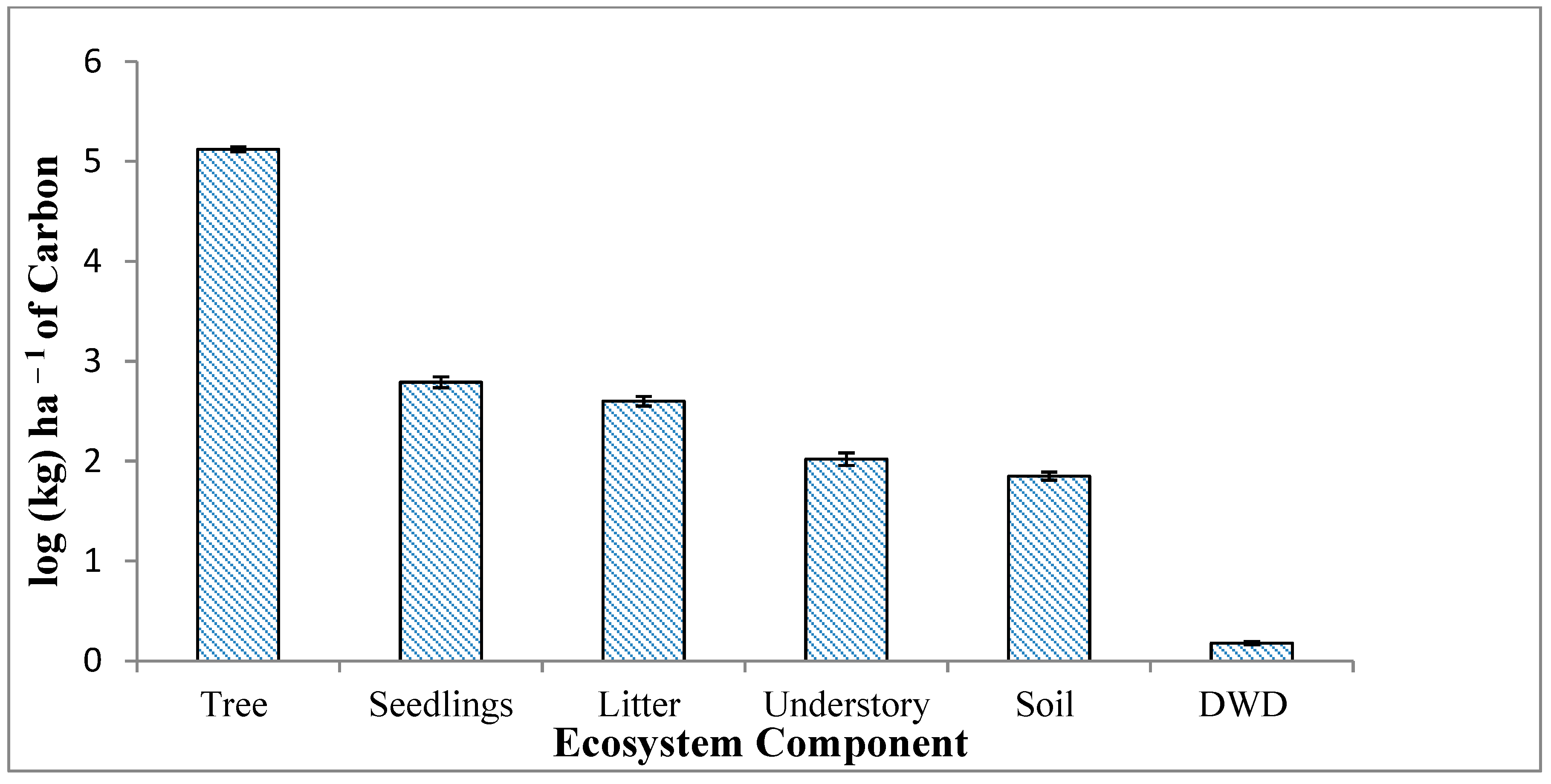
Total aboveground carbon stock for each vegetation component was calculated for the entire study area in terms of kg carbon per hectare (kg C ha−1) and later scaled to Mg (106 g) carbon per hectare (Mg C ha−1). Carbon stock per hectare was log transformed due to the disproportionate contribution by trees to the overall total carbon stock (Figure 4). The total carbon stock of all sampled “ecosystem components” [19] (trees, woody shrubs and seedlings, understory vegetation, DWD, soil, and leaf litter) in the 4.48 ha study area was 598.503 Mg C (133.594 Mg C ha−1). Trees dominated the carbon stock, contributing to 132.4 Mg C ha−1 (99%) of the estimated total stock. While standing dead trees (snags) were sporadically encountered, all outside the plots, we acknowledge the contribution to the total aboveground carbon stocks, albeit marginally so in our study site. However, studies have reported snags to contribute to 3.30 Mg ha−1 for oak–hickory stands and 5.80 Mg ha−1 for elm–ash–cottonwood stands of around 80–90 years old [56].

3.1.1. Trees

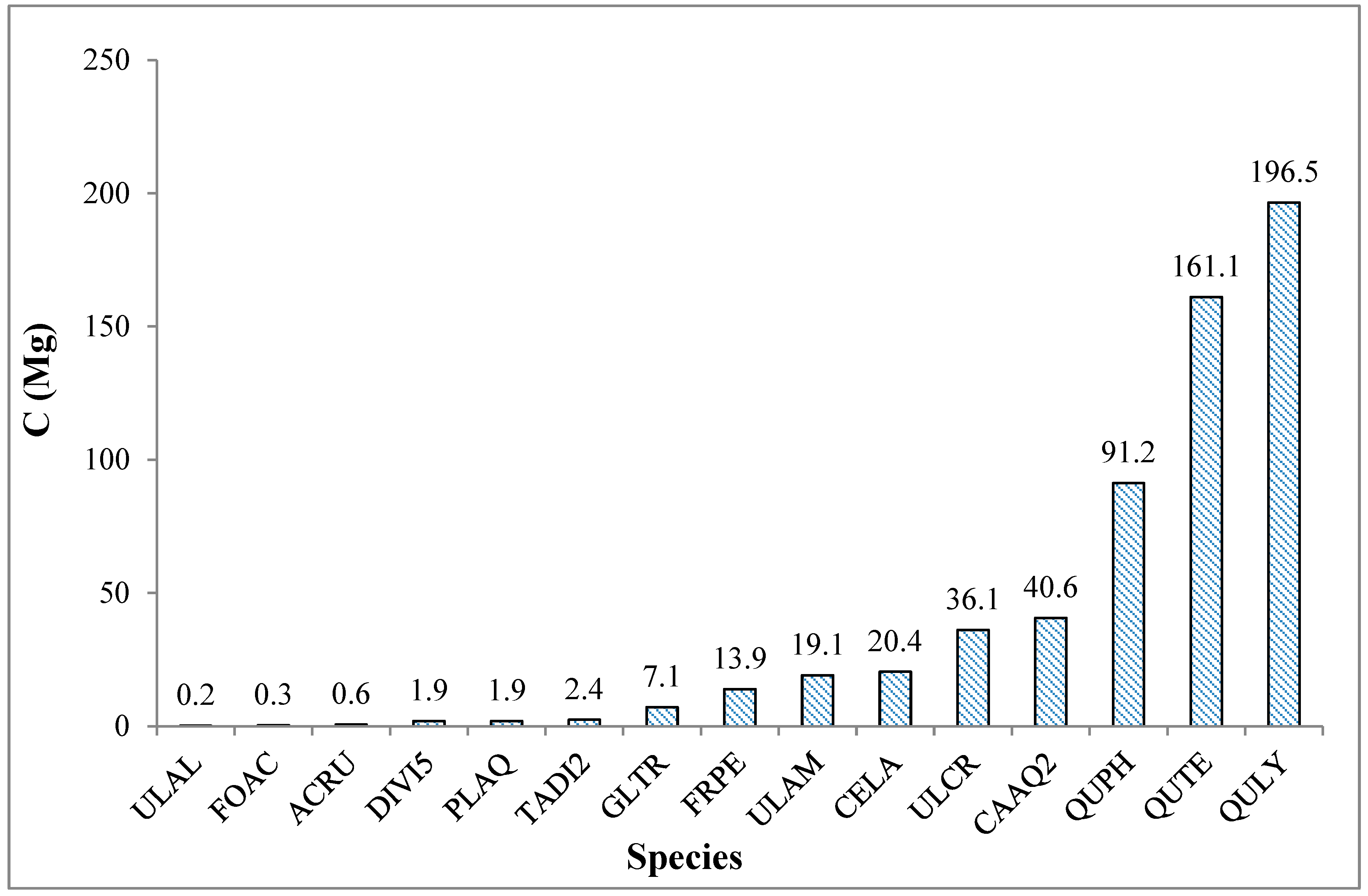
A total of 20 tree species, representing 13 families, were encountered during vegetation sampling, and a total of eight families representing 15 species were documented within density plot (15 m radius) boundaries (see Table S2). Stand density in the study area was calculated to be 311 stems ha−1. The total AGB (Table 2) and carbon stock (Figure 5) was calculated for each tree species. Overall, the total AGB and carbon stock for trees sampled was found to be 264.5 Mg ha−1 and 132.4 Mg C ha−1, respectively.
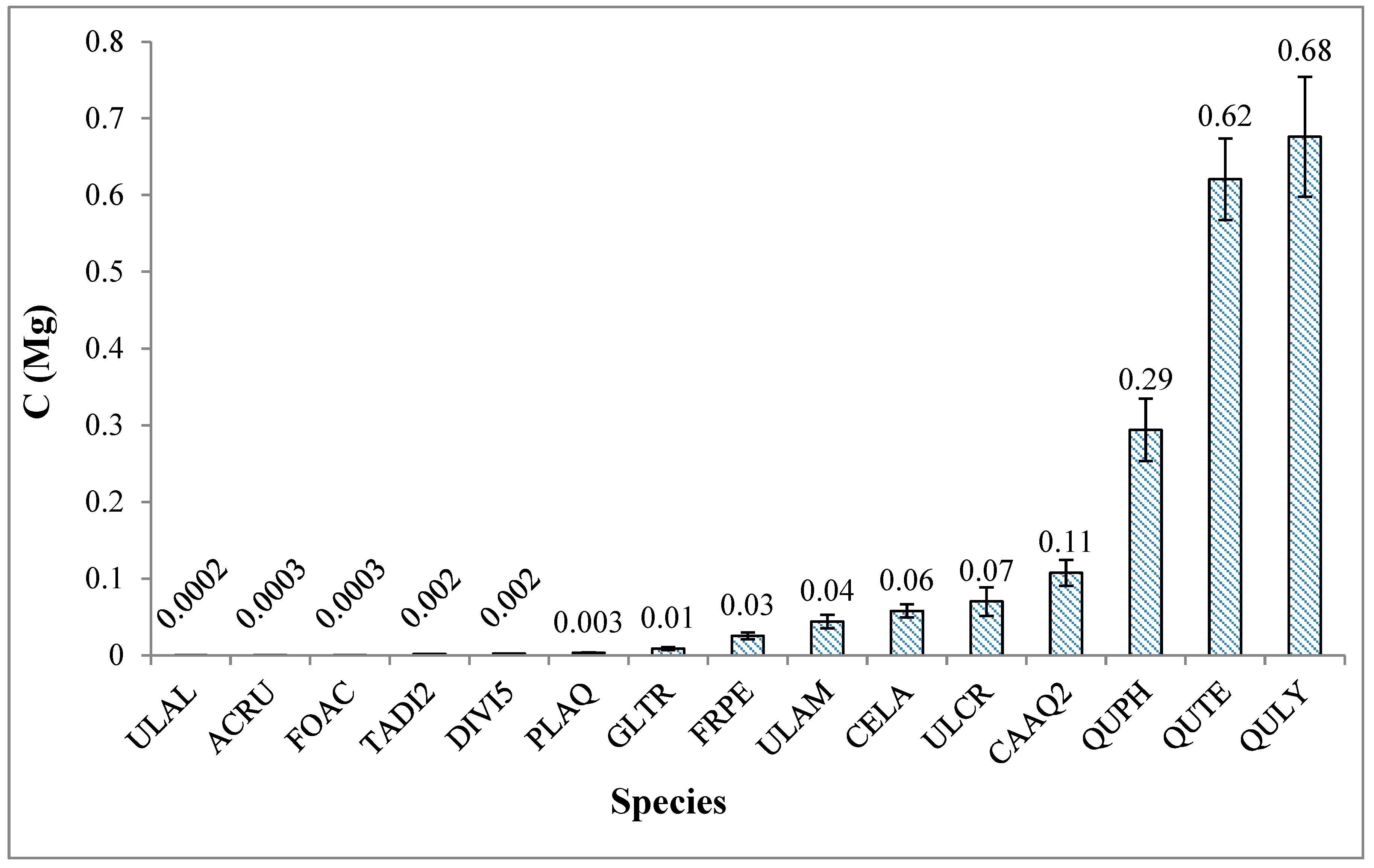
Some species were underrepresented in the sample; therefore, the average carbon stock per species was weighted by the number of each species sampled (Figure 6). The largest carbon stocks were contributed by Quercus lyrata, Quercus texana, and Quercus phellos (196.5, 161.1, and 91.2 Mg C, respectively), while Ulmus alata (0.2 Mg C) had the least. A similar trend was observed for carbon stocks per unit area with Quercus lyrata, Quercus texana, and Quercus phellos (43.9 Mg C ha−1, 36.0 Mg C ha−1, and 20.4 Mg C ha−1, respectively).

3.1.2. Woody Shrubs and Seedlings

Understory vegetation sampling recorded 33 species representing 21 families (see Table S3). The carbon stock (g C m−2) for each woody shrub and seedling species was calculated and then scaled to carbon stock per hectare (kg C ha−1). The total carbon stock of woody shrubs and seedlings was found to be 615.93 kg C ha−1 in the study area. Seedlings of Quercus phellos, Crataegus viridis, and Gleditsia triacanthos were found to be the dominant carbon stores, with 0.653 kg C ha−1, 0.595 kg C ha−1, and 0.41 kg C ha−1, respectively.

3.1.3. Understory Herbaceous Vegetation

The total AGB and carbon stock for understory herbaceous vegetation sampled in the study area were estimated to be 1440.9 g and 677.2 g C, respectively. Carbon stock per hectare was calculated to be 105.8 kg C ha−1 for all combined understory vegetation sampled.

3.1.4. Downed Woody Debris

The total AGB for CWD was calculated to be 0.011 kg ha−1. Total AGB for FWD of 0.6–2.5 cm and 2.5–7.5 cm size classes was 2.97 kg ha−1 and 0.043 kg ha−1, respectively. Carbon stock for CWD was calculated to be 0.006 kg C ha−1. Carbon stock was determined to be 1.482 kg C ha−1 and 0.021 kg C ha−1 for FWD of 0.6–2.5 cm and 2.5–7.5 cm size classes, respectively. Total DWD carbon stock was calculated to be 1.5 kg C ha−1.

3.1.5. Soil

The average bulk density (BD) of 16 soil samples was 1.10 g cm−3. The average percent organic carbon of the samples was 3.58% C. Total organic carbon of soil (0–25 cm depth) was calculated to be 7.13 g C m−2. Soil carbon stock was then scaled to kg C per hectare at 71.33 kg C ha−1.

3.1.6. Leaf Litter

The average AGB for 10 sacrificial plots was found to be 299.35 ± 36 g, with an average carbon content of 16.6% (0.166 g). In each sacrificial plot, leaf litter comprised 100% of the ground cover. Equation (9) was used to determine AGB (g m−2) for each 1 m2 plot. The total carbon stock of leaf litter was calculated to be 39.52 g C m−2 for all 64 1 m2 vegetation plots, which equals 395.2 kg C ha−1.

4. Discussion and Conclusions

Forested wetlands such as BHFs primarily store carbon in AGB and soil [57]. The vegetation structure [29,32] and high productivity [58] of BHFs increase the potential for carbon storage and therefore necessitate the quantification of carbon stores in such ecosystems. Approximately 99% (132.4 Mg C ha−1) of the total aboveground carbon for the RSWMA study area was stored in the tree component. The remaining 1% was distributed among leaf litter (395.2 kg C ha−1), understory herbaceous vegetation (105.8 kg C ha−1), soil (71.33 kg C m−2), seedlings (615.93 kg C ha−1), and DWD (1.51 kg C ha−1). The total AGB of trees (264.4 Mg ha−1) at the site was close to that reported in the Forest Inventory Analysis (FIA) for AGB estimates of oak–hickory forests (244.2 Mg ha−1). Therefore, it is evident that the total amount of AGB and associated carbon stock is primarily stored in trees, as expected since BHF ecosystems typically have sparse ground vegetation due to the flooding regime and fewer sciophytes. However, it should be noted that for this study, an estimate of 47% carbon stores was used for determining carbon stock in understory herbaceous vegetation, which is within the 41–47% range [40]. Although using the higher end of the reported range might have overestimated the carbon stock for this component, it is unlikely that these estimates would influence the overall carbon storage, since understory herbaceous vegetation accounted for less than 1% of the total forest carbon stock.
In comparison, the total aboveground carbon stock per hectare of the RSWMA is similar to that of other deciduous forests in the United States, especially in the distribution of carbon among forest components. Our findings concur with those of studies carried out at coastal plain forested wetlands in South Carolina [57], where the greatest carbon storage in these ecosystems is in trees. However, reports of research from a Panamanian tropical moist forest [12] indicated that only 41% of the system’s carbon stock was in trees. This could be due to the dense under-canopy and ground vegetation present in such forests.
Forested systems tend to store large amounts of carbon in their tree components, with the remaining carbon being distributed among soil, understory vegetation, DWD, and leaf litter differently depending on the ecosystem [59]. The BHF ecosystem of the RSWMA can expectedly differ from these previously mentioned studies as the carbon stock amounts per ecosystem component will differ from the forest type and vegetation [59]. Kirby and Potvin (2003) [12] reported greater overall storage in understory vegetation and woody debris compared to that found in the RSWMA, and a transition of dominant carbon storage in understory vegetation to trees was observed with an increase in forest age. The large contribution of tree carbon to the total carbon stock of the site could be an artifact of stand maturity and the dominance of overstory trees [60,61].
When the carbon stock of trees only in the site was examined, a significant difference in total carbon stored among species was observed. The genus Quercus dominated the carbon stock among all other tree genera, accounting for approximately 76% of the overall carbon stored in trees for the sampled site. The species Celtis laevigata and Carya aquatica and the genus Ulmus were the next largest stores of carbon, accounting for approximately 3.5%, 7%, and 9% of the total tree carbon, respectively. Although the contribution of each species was weighted to account for trees that may have been underrepresented, Quercus contained more stored carbon than any other genus. The RSWMA is considered an oak–hickory dominant BHF association, and it can therefore be expected that Quercus, Carya, and Ulmus would contain more carbon compared to other species in the site.
The second largest store of carbon, 615.93 kg C ha−1, was in woody shrubs and seedlings, albeit only 0.5% of the total. This is because relatively sparse vegetation capable of tolerating these flood-shade conditions in bottomlands can be established in such BHFs.
The third most important carbon store at 0.3% (395.2 kg C ha−1) was leaf litter. Due to the dominance of the site by overstory tree species, it was expected that leaf litter would also constitute relatively high levels of carbon storage, although only a small fraction of the total. As suggested by [62], foliage AGB and its potential effects on forest carbon should not be undermined, especially in systems where the dominant vegetation component is large trees, as supported by the findings in this site.
Wetland soils are thought to be potentially large stores of carbon [63]. This storage of carbon can be closely related to the inputs from leaf litter and DWD. As leaf litter and DWD decay, the dead plant material contributes to soil organic matter and subsequently soil carbon [59]. In this study, we carried out an on-site rate of decomposition experiment using leaves from three predominant tree genera—Carya sp., Ulmus sp., and Quercus sp. Decomposition rates were calculated by allowing leaf samples to decompose for 90 days. The mean decomposition rate for the study area was estimated to be −0.004 g day−1. Therefore, input from a 395.2 kg C ha−1 leaf litter pool has the potential to add large amounts of organic carbon to the site’s soil pool. Although the carbon stock of DWD was the smallest pool of carbon for the site, its contribution to the soil carbon stock should be accounted for. Future research that dedicates efforts to the analysis of the decomposition rate of DWD could offer insight into carbon inputs for BHF soils in the site.
The planar intersect method was efficient for estimating the volume and AGB of wood debris. However, sites that experience flooding, such as the RSWMA, may experience events where DWD from the ground may be relocated by flood waters. The RSWMA is bordered on the south by a small levee. Since the plots to the southwest of the study site had higher DWD values, we suspect that this distribution may have been due to the natural hydrology of the site. Future research in BHFs needs to include the determination of decay classes for DWD. The carbon stock of DWD fluctuates according to the decay class and this may lead to an overestimation of the carbon stock by not accounting for a carbon reduction based on stages of decay.
The total carbon stock estimated for the BHF ecosystem at the RSWMA is 133 Mg C ha−1, comparable to estimates of 131 Mg C ha−1 [19] for the south-central region (including Louisiana), 170 Mg C ha−1 [64] for Continental US forests, and estimates of 155 Mg C ha−1 [65] for temperate forests. While our results are comparable to the regional values, the estimates derived in this study were lower than values reported at the continental and biome levels. This could potentially be because we did not take into account the carbon stored in snags, which may contribute significantly to the total carbon stock in this forest, albeit in smaller proportions. Putting aside the trade-offs associated with large-scale estimates such as the one mentioned above, we can reasonably infer that the RSWMA is comparable to other temperate forests of the conterminous US in terms of carbon stock per hectare. In light of the findings of this study, carbon storage is yet another ecosystem service that can be added to the repertoire of this unique ecosystem and the vital role it plays in shaping global carbon stocks.

Supplementary Materials

The following supporting information can be downloaded at: https://www.mdpi.com/article/10.3390/f14050974/s1, Table S1: Biomass equations used for tree species sampled within 15 m radius plots; Table S2: List of trees and woody species in Russell Sage Wildlife Management Area; Table S3: List of understory vegetation in Russell Sage Wildlife Management Area.

Author Contributions

Conceptualization, J.R.S. and J.B.; methodology, J.R.S. and J.B.; data analysis, J.R.S., J.B. and B.K.; writing—reviewing and editing, J.R.S., J.B. and B.K. All authors have read and agreed to the published version of the manuscript.

Funding

This research was funded by the Louisiana Board of Regents [LEQSF-ENH-TR-33].

Institutional Review Board Statement

Not applicable.

Informed Consent Statement

Not applicable.

Data Availability Statement

The datasets generated and/or analyzed during the current study are available from the corresponding author on request.

Acknowledgments

We are grateful to Matthew Herron and Matthew Reid for their assistance in plot setup and fieldwork. Jenaé Clay and Stephanie Olmstead helped with fieldwork and data collection.

Conflicts of Interest

The authors declare no conflict of interest.

References

  1. Nordhaus, W.D. Can We Control Carbon Dioxide? (From 1975). Am. Econ. Rev. 2019, 109, 2015–2035. [Google Scholar] [CrossRef]
  2. Lemon, E.R. (Ed.) CO2 and Plants: The Response of Plants to Rising Levels of Atmospheric Carbon Dioxide; CRC Press: Boca Raton, FL, USA, 2019. [Google Scholar]
  3. Snæbjörnsdóttir, S.; Sigfússon, B.; Marieni, C.; Goldberg, D.; Gislason, S.R.; Oelkers, E.H. Carbon dioxide storage through mineral carbonation. Nat. Rev. Earth Environ. 2020, 1, 90–102. [Google Scholar] [CrossRef]
  4. Cheng, W.; Dan, L.; Deng, X.; Feng, J.; Wang, Y.; Peng, J.; Tian, J.; Qi, W.; Liu, Z.; Zheng, X.; et al. Global monthly gridded atmospheric carbon dioxide concentrations under the historical and future scenarios. Sci. Data 2022, 9, 83. [Google Scholar] [CrossRef]
  5. Mildrexler, D.J.; Berner, L.T.; Law, B.E.; Birdsey, R.A.; Moomaw, W.R. Large Trees Dominate Carbon Storage in Forests East of the Cascade Crest in the United States Pacific Northwest. Front. For. Glob. Chang. 2020, 3, 127. [Google Scholar] [CrossRef]
  6. Chen, L.-C.; Guan, X.; Li, H.-M.; Wang, Q.-K.; Zhang, W.-D.; Yang, Q.-P.; Wang, S.-L. Spatiotemporal patterns of carbon storage in forest ecosystems in Hunan Province, China. For. Ecol. Manag. 2018, 432, 656–666. [Google Scholar] [CrossRef]
  7. Hofhansl, F.; Chacón-Madrigal, E.; Fuchslueger, L.; Jenking, D.; Morera-Beita, A.; Plutzar, C.; Silla, F.; Andersen, K.M.; Buchs, D.M.; Dullinger, S.; et al. Climatic and edaphic controls over tropical forest diversity and vegetation carbon storage. Sci. Rep. 2020, 10, 1–11. [Google Scholar] [CrossRef]
  8. Dalmonech, D.; Marano, G.; Amthor, J.S.; Cescatti, A.; Lindner, M.; Trotta, C.; Collalti, A. Feasibility of enhancing carbon sequestration and stock capacity in temperate and boreal European forests via changes to management regimes. Agric. For. Meteorol. 2022, 327, 109203. [Google Scholar] [CrossRef]
  9. Bouchard, V.; Cochran, M. Wetlands: Carbon Sequestration. Managing Water Resources and Hydrological Systems; CRC Press: Boca Raton, FL, USA, 2020; pp. 715–719. [Google Scholar]
  10. Aguilos, M.; Mitra, B.; Noormets, A.; Minick, K.; Prajapati, P.; Gavazzi, M.; Sun, G.; McNulty, S.; Li, X.; Domec, J.C.; et al. Long-term carbon flux and balance in managed and natural coastal forested wetlands of the Southeastern USA. Agric. For. Meteorol. 2020, 288–289, 108022. [Google Scholar] [CrossRef]
  11. Panja, P. Deforestation, Carbon dioxide increase in the atmosphere and global warming: A modelling study. Int. J. Model. Simul. 2019, 41, 209–219. [Google Scholar] [CrossRef]
  12. Kirby, K.R.; Potvin, C. Variation in carbon storage among tree species: Implications for the management of a small-scale carbon sink project. For. Ecol. Manag. 2007, 246, 208–221. [Google Scholar] [CrossRef]
  13. Ordóñez, J.; de Jong, B.; García-Oliva, F.; Aviña, F.; Pérez, J.; Guerrero, G.; Martínez, R.; Masera, O. Carbon content in vegetation, litter, and soil under 10 different land-use and land-cover classes in the Central Highlands of Michoacan, Mexico. For. Ecol. Manag. 2008, 255, 2074–2084. [Google Scholar] [CrossRef]
  14. Sarwar, S.; Waheed, R.; Farooq, M.U.; Sarwar, S. Investigate solutions to mitigate CO2 emissions: The case of China. J. Environ. Plan. Manag. 2022, 65, 2054–2080. [Google Scholar] [CrossRef]
  15. Nair, P.K.R.; Kumar, B.M.; Nair, V.D. Agroforestry as a strategy for carbon sequestration. J. Plant Nutr. Soil Sci. 2009, 172, 10–23. [Google Scholar] [CrossRef]
  16. Sharma, T.; Kurz, W.A.; Stinson, G.; Pellatt, M.G.; Li, Q. A 100-year conservation experiment: Impacts on forest carbon stocks and fluxes. For. Ecol. Manag. 2013, 310, 242–255. [Google Scholar] [CrossRef]
  17. Bastin, J.F.; Finegold, Y.; Garcia, C.; Mollicone, D.; Rezende, M.; Routh, D.; Zohner, C.M.; Crowther, T.W. The global tree restoration potential. Science 2019, 365, 76–79. [Google Scholar] [CrossRef]
  18. Zhang, X.M.; Brandt, M.; Yue, Y.M.; Tong, X.W.; Wang, K.L.; Fensholt, R. The Carbon Sink Potential of Southern China After Two Decades of Afforestation. Earth’s Future 2022, 10, e2022EF002674. [Google Scholar] [CrossRef]
  19. Birdsey, R. Carbon Storage and Accumulation in United States Forest Ecosystems. General Technical Report WO-59; US Department of Agriculture, Forest Service, Washington Office: Washington, DC, USA, 1992; Volume 59, 51p. [Google Scholar]
  20. Jenkins, J.; Chojnacky, D.; Heath, L.; Birdsey, R. National-scale biomass estimators for United States tree species. For. Sci. 2003, 49, 12–35. [Google Scholar]
  21. Shoch, D.; Kaster, G.; Hohl, A.; Souter, R. Carbon storage of bottomland hardwood afforestation in the Lower Mississippi Valley, USA. Wetlands 2009, 29, 535–542. [Google Scholar] [CrossRef]
  22. Kuimi, V.; Jayakumar, S. Methods to Estimate Above-Ground Biomass and Carbon Stock in Natural Forests—A Review. J. Ecosyst. Ecography 2012, 2, 1–7. [Google Scholar] [CrossRef]
  23. Omasa, K.; Qiu, G.Y.; Watanuki, K.; Yoshimi, K.; Akiyama, Y. Accurate Estimation of Forest Carbon Stocks by 3-D Remote Sensing of Individual Trees. Environ. Sci. Technol. 2003, 37, 1198–1201. [Google Scholar] [CrossRef]
  24. Campbell, A.D.; Fatoyinbo, T.; Charles, S.P.; Bourgeau-Chavez, L.L.; Goes, J.; Gomes, H.; Halabisky, M.; Holmquist, J.; Lohrenz, S.; Mitchell, C.; et al. A review of carbon monitoring in wet carbon systems using remote sensing. Environ. Res. Lett. 2022, 17, 025009. [Google Scholar] [CrossRef]
  25. Pan, Y.; Luo, T.; Birdsey, R.; Hom, J.; Melillo, J. ‘New Estimates of Carbon Storage and Sequestration in China’s Forests: Effects of Age—Class and Method on Inventory-Based Carbon Estimation’. Clim. Chang. 2004, 67, 211–236. [Google Scholar]
  26. Chave, J.; Andalo, C.; Brown, S.; Cairns, M.A.; Chambers, J.Q.; Eamus, D.; Fölster, H.; Fromard, F.; Higuchi, N.; Kira, T.; et al. Tree allometry and improved estimation of carbon stocks and balance in tropical forests. Oecologia 2005, 145, 87–99. [Google Scholar] [CrossRef]
  27. Wondrade, N.; Dick, O.B.; Tveite, H. Estimating aboveground biomass and carbon stock in the Lake Hawassa Watershed, Ethiopia by integrating remote sensing and allometric equations. For. Res. 2015, 4, 2. [Google Scholar]
  28. Ao, A.; Changkija, S.; Brearley, F.Q.; Tripathi, S.K. Plant Community Composition and Carbon Stocks of a Community Reserve Forest in North-East India. Forests 2023, 14, 245. [Google Scholar] [CrossRef]
  29. Stanturf, J.A.; Schweitzer, C.; Gardiner, E. Afforestation of marginal agricultural land in the Lower Mississippi River Alluvial Valley, USA. Silva Fenn. 1998, 32, 281–297. [Google Scholar] [CrossRef]
  30. Gardiner, E.; Oliver, J. Restoration of Bottomland Hardwood Forests in the Lower Mississippi Alluvial Valley, USA. In Restoration of Boreal and Temperate Forests. Restoration of Bottomland Hardwood Forests in the Lower Mississippi Alluvial Valley; Stanturf, J.A., Madsen, P., Eds.; CRC Press: Boca Raton, FL, USA, 2005; pp. 235–251. [Google Scholar]
  31. Wilson, R.R.; Oliver, J.M.; Twedt, D.J.; Uihlein, W.B. Bottomland hardwood restoration in the Mississippi Alluvial Valley: Looking past the trees to see the forest. Ecol. Manag. Bottomland Hardwood Syst. State Our Underst. 2005, 10, 519–532. [Google Scholar]
  32. Dey, D.C.; Gardiner, E.S.; Kabrick, J.M.; Stanturf, J.A.; Jacobs, D.F. Innovations in afforestation of agricultural bottomlands to restore native forests in the eastern USA. Scand. J. For. Res. 2010, 25 (Suppl. S8), 31–42. [Google Scholar] [CrossRef]
  33. Schmidt, J.; Moore, R.; Alber, M. Integrating ecosystem services and local government finances into land use planning: A case study from coastal Georgia. Landsc. Urban Plan. 2014, 122, 56–67. [Google Scholar] [CrossRef]
  34. Hodges, J. Ecology of Bottomland Hardwoods. In A Workshop to Resolve Conflicts in the Conservation of Migratory Landbirds in Bottomland Hardwood Forests; USDA Forest Service: New Orleans, LA, USA, 1994; p. 5. [Google Scholar]
  35. Reid, M.L. A Quarter Century of Plant Succession in a Bottomland Hardwood Forest in Northeastern Louisiana. MS Biology Dissertation, University of Louisiana Monroe, Monroe, LA, USA, 2014. [Google Scholar]
  36. King, S.L.; Keim, R.F. Hydrologic Modifications Challenge Bottomland Hardwood Forest Management. J. For. 2019, 117, 504–514. [Google Scholar] [CrossRef]
  37. Wharton, C.H.; Kitchens, W.M.; Sipe, T.W. Ecology of Bottomland Hardwood Swamps of the Southeast: A Community Profile; (No., FWS/OBS-81/37); Institute of Ecology, Georgia University: Athens, GA, USA; Fish and Wildlife Service, National Coastal Ecosystems Team: Slidell, LA, USA; Department of Biology, Wabash College: Crawfordsville, IN, USA, 1982. [Google Scholar]
  38. Louisiana Department of Wildlife and Fisheries. Louisiana Comprehensive Wildlife Louisiana Comprehensive Wildlife Conservation; Louisiana Department of Wildlife and Fisheries: Baton Rouge, LA, USA, 2005. [Google Scholar]
  39. Guimbellot, T. Analysis of Woody Plants on the Russell Sage Wildlife Management Area. Doctoral Dissertation, Northeast Louisiana University, Monroe, LA, USA, 1990. [Google Scholar]
  40. Law, B.; Arkebauer, T.; Campbell, J.; Chen, J.; Sun, O.; Schwartz, M.; van Ingen, C.; Verma, S. Terrestrial Carbon Observations: Protocols for Vegetation Sampling and Data Submission; FAO: Rome, Italy, 2008. [Google Scholar]
  41. Giese, L.A.B. Carbon Pools and Fluxes as an Indicator of Riparian Restoration; Virginia Polytechnic Institute and State University: Blacksburg, VA, USA, 2001. [Google Scholar]
  42. Tritton, L.; Hornbeck, J. Biomass Equations for Major Tree Species of the Northeast; US Department of Agriculture, Forest Service, Northeastern Forest Experiment Station: Upper Darby, PA, USA, 1982. [Google Scholar]
  43. Jenkins, J.C.; Chojnacky, D.; Heath, L.; Birdsey, R. Comprehensive Database of Diameter-Based Biomass Regressions for North American Tree Species; General Technical Report NE-319; United States Department of Agriculture, Forest Service: Washington, DC, USA, 2004. [Google Scholar]
  44. Henry, M.; Bombelli, A.; Trotta, C.; Alessandrini, A.; Birigazzi, L.; Sola, G.; Vieilledent, G.; Santenoise, P.; Longuetaud, F.; Valentini, R.; et al. GlobAllomeTree: International platform for tree allometric equations to support volume, biomass and carbon assessment. iForest Biogeosciences For. 2013, 6, 326–330. [Google Scholar] [CrossRef]
  45. Brown, S. Estimating Biomass and Biomass Change of Tropical Forests: A Primer; Food & Agriculture Org.: Rome, Italy, 1997; Volume 134, p. 72. Available online: http://books.google.com/books?id=uv-ISezvitwC (accessed on 19 September 2019).
  46. Jain, T.B.; Graham, R.T.; Adams, D. Carbon Concentrations and Carbon Pool Distributions in Dry, Moist, and Cold Mid-Aged Forests of the Rocky Mountains. In Integrated Management of Carbon Sequestration and Biomass Utilization Opportunities in a Changing Climate: Proceedings of the 2009 National Silviculture Workshop, Boise, Idaho, 15–18 June 2009; ID. Proceedings RMRS-P-61; Jain, T.B., Graham, R.T., Sandquist, J., Eds.; US Department of Agriculture, Forest Service, Rocky Mountain Research Station: Fort Collins, CO, USA, 2009; Volume 61, pp. 39–59. [Google Scholar]
  47. Woodall, C.W.; Monleon, V.J. Sampling Protocol, Estimation, and Analysis Procedures for the Down Woody Materials Indicator of the FIA Program; Volume 256 of General technical report NC NRS-22; USDA Forest Service, North Central Research Station: Newtown Square, PA, USA, 2008; Volume 22, 68p. [Google Scholar]
  48. Harmon, M.E.; Fasth, B.; Woodall, C.W.; Sexton, J. Carbon concentration of standing and downed woody detritus: Effects of tree taxa, decay class, position, and tissue type. For. Ecol. Manag. 2013, 291, 259–267. [Google Scholar] [CrossRef]
  49. Burt, R. Soil Survey Laboratory Methods Manual, Soil Survey Investigation Report; U.S. Department of Agriculture Natural Resources Conservation Service National Soil Survey Center: Lincoln, NE, USA, 2004; Volume 42. [Google Scholar]
  50. Lunt, H. The carbon-organic matter factor in forest soil humus. Soil Sci. 1931, 32, 27–34. [Google Scholar] [CrossRef]
  51. Schumacher, B.A. Methods for the Determination of Total Organic Carbon (TOC) in Soils and Sediments; United States Environmental Protection Agency Environmental Sciences Division National Exposure Research Laboratory: Las Vegas, NV, USA, 2002; pp. 1–23. [Google Scholar]
  52. Adams, M.B.; Angradi, T.R. Decomposition and nutrient dynamics of hardwood leaf litter in the Femow Whole-Watershed Acidification Experiment. For. Ecol. Manag. 1996, 1127, 61–69. [Google Scholar] [CrossRef]
  53. Chaiyo, U.; Pizzo, Y.; Garivait, S. Estimation of Carbon Released from Dry Dipterocarp Forest Fires in Thailand. Int. J. Environ. Ecol. Geol. Min. Eng. 2013, 7, 611–614. [Google Scholar]
  54. Mamoun, E.M.; Idris, E.Z.; Ibrahim, E.M. Modelling Height-Diameter Relationships of Selected Economically Important Natural Forests Species. J. For. Prod. Ind. 2013, 2, 34–42. [Google Scholar]
  55. USDA. The Plants Database; National Plant Data Team: Greensboro, NC, USA, 2019. Available online: http://plants.usda.gov (accessed on 16 September 2019).
  56. Smith, J.E. Methods for Calculating Forest Ecosystem and Harvested Carbon with Standard Estimates for Forest Types of the United States (No. 343); United States Department of Agriculture, Forest Service, Northeastern Research Station: Newtown Square, PA, USA, 2006. [Google Scholar]
  57. Giese LAust, W.; Kolka, R.; Trettin, C. Biomass and carbon pools of disturbed riparian forests. For. Ecol. Manag. 2003, 180, 493–508. [Google Scholar] [CrossRef]
  58. Trettin, C.C.; Jurgensen, M.F. Carbon Cycling in Wetland Forest Soils; Lewis Publishers: Boca Raton, FL, USA, 2003; pp. 311–331. [Google Scholar]
  59. Chapin, S.I.; Matson, P.A.; Mooney, H.A. Principles of Terrestrial Ecosystem Ecology; Springer Science & Business Media: Berlin/Heidelberg, Germany, 2011; 529p. [Google Scholar]
  60. Falk, M.; Wharton, S.; Schroeder, M.; Ustin, S.; Paw, U.T. Flux partitioning in an old-growth forest: Seasonal and interannual dynamics. Tree Physiol. 2008, 28, 509–520. [Google Scholar] [CrossRef]
  61. Stephenson, N.; Das, A.J.; Condit, R.; Russo, S.; Baker, P.; Beckman, N.; Coomes, D.A.; Lines, E.R.; Morris, W.K.; Rüger, N.; et al. Rate of tree carbon accumulation increases continuously with tree size. Nature 2014, 507, 90–93. [Google Scholar] [CrossRef]
  62. Grote, R. Foliage and branch biomass estimation of coniferous and deciduous tree species. Silva Fenn. 2002, 36, 779–788. [Google Scholar] [CrossRef]
  63. Miao, G.; Noormets, A.; Domec, J.-C.; Trettin, C.C.; McNulty, S.; Sun, G.; King, J.S. The effect of water table fluctuation on soil respiration in a lower coastal plain forested wetland in the southeastern U.S. J. Geophys. Res. Biogeosci. 2013, 118, 1748–1762. [Google Scholar] [CrossRef]
  64. Dixon, R.K.; Solomon, A.M.; Brown, S.; Houghton, R.A.; Trexier, M.C.; Wisniewski, J. Carbon Pools and Flux of Global Forest Ecosystems. Science 1994, 263, 185–190. [Google Scholar] [CrossRef]
  65. Pan, Y.; Birdsey, R.A.; Fang, J.; Houghton, R.; Kauppi, P.E.; Kurz, W.A.; Phillips, O.L.; Shvidenko, A.; Lewis, S.L.; Canadell, J.G.; et al. A Large and Persistent Carbon Sink in the World’s Forests. Science 2011, 333, 988–993. [Google Scholar] [CrossRef]
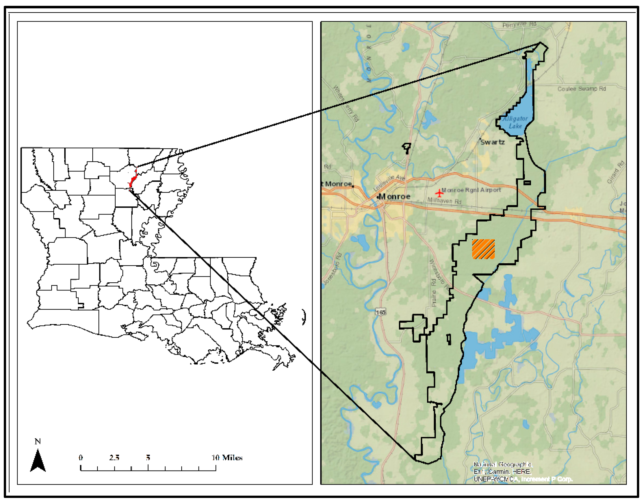
Figure 1. Map of Louisiana, showing the location of Russell Sage Wildlife Management Area (black border) in the northeast. The hatched area on the right indicates the location of the study site. (Basemap source: Esri Canada. “Topographic/Topographie” [Web Map]. Scale Not Given. “National Geographic World”. 4 May 2023. Developed in ArcGIS [ArcMap] Version 10.8.1.)
Forests 14 00974 g001
Figure 2. (a) Study design depicting the plot placement within a site. Within the four areas, there were 16 sites and 64 plots (15 m radius). (b) Detailed sampling design depicting the 15 m radius plot for sampling trees, 5 m radius subplot for estimation of understory cover, 2 m radius subplot for sampling shrubs and woody seedlings, 1 m2 subplot for estimating ground cover and VOM, and two intersecting transects (30 m) for sampling downed woody debris (DWD) in the study site at Russel Sage Wildlife Management Area in Northeast Louisiana.
Forests 14 00974 g002
Figure 3. Regression model predicting tree height from DBH using 896 trees measured in Russell Sage Wildlife Management Area in Northeast Louisiana.
Forests 14 00974 g003
Figure 4. Average carbon stock (log) of each sampled ecosystem component in the Russel Sage Wildlife Management Area in Northeast Louisiana. Error bars represent log-transformed standard error (1SD) values.
Forests 14 00974 g004
Figure 5. Total carbon stock for all tree species sampled within the 64 15 m radius plots in the Russell Sage Wildlife Management Area in Northeast Louisiana.
Forests 14 00974 g005
Figure 6. Average estimated carbon stock by species sampled in Russell Sage Wildlife Management Area in Ouachita Parish, Louisiana. Error bars indicate 1 standard deviation.
Forests 14 00974 g006
Table 1. Species-specific equations for estimating tree height based on DBH for trees sampled in Russell Sage Wildlife Management Area, Northeast Louisiana. The alphanumeric acronyms used for species are standard codes assigned by USDA, NRCS for all plant taxa.
Species-Specific Height Equations
SpeciesNEquationR2
ACRU9H = 4.5844 × ln(DBH) + 0.25780.8624
CAAQ2142H = 6.2917 × ln(DBH) − 3.45390.8232
CELA56H = 5.3685 × ln(DBH) − 1.20170.7894
CEOC210H = 3.4878 × ln(DBH) − 1.17390.5880
COFO1N/A due to sample size-
CRVI22N/A due to sample size-
DIVI535H = 5.5713 × ln(DBH) − 1.12840.8452
FOAC37H = 2.8701 × ln(DBH) + 0.83980.5749
FRPE57H = 5.0789 × ln(DBH) − 1.08960.8548
GLTR15H = 8.1933 × ln(DBH) − 7.01030.8993
ILDE71H = 2.3271 × ln(DBH) + 1.42270.5935
PLAQ11H = 5.0546 × ln(DBH) − 2.89410.9338
QULY138H = 8.0379 × ln(DBH) − 7.00090.7805
QUTE131H = 8.4535 × ln(DBH) − 8.6580.6064
QUPH68H = 7.7845 × ln(DBH) − 3.8180.6277
STAM45H = 3.6215 × ln(DBH) + 0.68960.8828
TADI21N/A due to sample size-
ULAL21H = 4.0795 × ln(DBH) − 1.02970.7952
ULAM27H = 7.3993 × ln(DBH) − 7.3550.7553
ULCR59H = 6.3431 × ln(DBH) − 4.8230.8655
Table 2. Height, DBH, AGB, and carbon stock of each species sampled in Russell Sage Wildlife Management Area, Northeast Louisiana. The alphanumeric acronyms used for species are standard codes assigned by USDA, NRCS for all plant taxa.
SpeciesAverage Height (m)# IndividualsAverage DBH (cm)Total Biomass (Mg)Total Carbon (Mg)
ACRU5.4815.91.10.6
CAAQ25.621820.381.140.6
CELA11.11662040.820.4
DIVI56.62716.63.71.9
FOAC3.8321.20.60.3
FRPE7.38423.927.913.9
GLTR15.61730.914.27.1
PLAQ6.92019.53.91.9
QULY22.826936.9392.1196.5
QUTE22.731235321.6161.1
QUPH25.69047.3182.391.2
TADI223.8177.54.72.4
ULAL6.2513.10.30.2
ULAM14.511921.638.119.1
ULCR8.9571872.236.1
Disclaimer/Publisher’s Note: The statements, opinions and data contained in all publications are solely those of the individual author(s) and contributor(s) and not of MDPI and/or the editor(s). MDPI and/or the editor(s) disclaim responsibility for any injury to people or property resulting from any ideas, methods, instructions or products referred to in the content.