Research on the Identification of Particleboard Surface Defects Based on Improved Capsule Network Model

Abstract

Aiming at the problems of low classification accuracy and overfitting caused by the limited number of particleboard image samples, a Capsule Network algorithm based on the improved CBAM (Convolutional Block Attention Module) attention model is proposed. The improved algorithm utilizes the GELU equation to improve the CBAM attention model and incorporates it into the convolutional layer of the Capsule Network. In this way, the improved algorithm optimizes the feature maps of surface defects and, meanwhile, improves the training efficiency and stability of the model. The improved algorithm alleviates the overfitting problem by adding a dropout layer, which makes the model more suitable for small sample classification. The effectiveness of the method proposed in this paper is verified by classification experiments on the dataset of particleboard surface defect images.

1. Introduction

Particleboard, also known as bagasse board, is one of the three main products of man-made board at present. Particleboard is a kind of wood-based panel made of wood or other lignocellulosic materials, which is glued under the action of heat and pressure after applying adhesive. The raw materials of particleboard come from a wide range of sources, and the board has high strength. The sales market of particleboard-related products is also broad [1].

At present, there are many kinds of automatic production equipment for particleboard, among which the continuous flat press is the leading technology. It has the advantages of high automation and outstanding production capacity. However, due to the particularity of the raw material source of particleboard, there are some problems in the production line of the continuous flat press. Due to factors such as uneven size and type of raw materials, machine errors in production equipment, and workshop environmental interference, individual products may have surface defects. These defects can impact the subsequent veneer process, the appearance and quality of the finished board, and make secondary processing more challenging. With the refinement and high-end development of the furniture manufacturing industry, the demand for high-quality particleboard is rising. Consequently, particleboard manufacturers pay more attention to product surface quality testing than ever before, making it one of the core measurement factors for board grading. Among the available quality testing methods, surface defect image classification is a critical component for improving the quality of particleboard products.

During the particleboard production process, surface quality inspection is a crucial step that greatly impacts the subsequent veneer and edge bonding processes. The influence of surface defects on the board quality can vary widely depending on factors such as the damage degree, the defect type, and the defect area [2]. Currently, the treatment schemes usually involve either leaving the defect untreated or directly cutting the defective parts of the board. The former approach often leads to problems such as blistering and layering of the board after veneering, thereby affecting the quality of the final product and subsequent processing. The latter approach can result in the wastage of raw materials and production resources, which is not conducive to the effective utilization of wood resources. Detecting and identifying surface defects on the board and implementing different treatment methods based on the detection and identification results can address the aforementioned issues.

With the development of industrial technology, non-destructive testing methods are emerging as a replacement for manual operations in detecting and identifying defects in industrial products. In the wood-based panel industry, researchers have been exploring defect detection technology, resulting in progress in non-destructive testing and identification methods. These methods include ultrasonic detection [3], X-ray detection [4], and machine vision detection [5]. Ultrasonic testing uses ultrasonic propagation attenuation law to judge the defect position in the panel, but it has drawbacks such as long detection time, the need for coupling agents, and operator experience. X-ray testing targets internal defects in the panel, utilizing ray beam attenuation imaging to display the defect size and position. However, protective equipment is required due to the harmful effects of radiation, limiting its applicability in open production environments.

Machine vision technology emerged in the 1970s and 1980s, owing to the progress of digital image processing and computer pattern recognition technologies. In the realm of product surface defect detection, this technology acquires product surface images through detection and perception and subsequently produces results of diverse projects such as defect measurement, classification, and quality evaluation based on algorithms. It is capable of multi-mode detection, such as quantitative, qualitative, and semi-quantitative. This method is highly suitable for industrial production fields associated with panel defect detection due to its fast detection speed, flexible processing, high accuracy, and easy equipment configuration. However, the industrial production line’s production environment is intricate, and the requirements for surface defect detection differ for different boards. Thus, surface defect detection and recognition technology based on machine vision still present extensive research prospects.

In the problem of surface defect detection and recognition based on machine vision, extracting the defect features to form a sample set, building a defect-type classifier, training the classifier, and classifying the defects according to their feature values are necessary. Currently, the main classifiers are the Bayesian Classifier, K-Nearest Neighbor Classifier, Decision Tree Classifier, Random Forest Classifier, Support Vector Machine Classifier, and Neural Network Classifier. Scholars have conducted much in-depth research and innovations on relevant issues in recent years [6,7,8,9,10,11]. He, T and Liu, Y used the improved AP (Affinity Propagation) clustering algorithm and SOM (Self-Organizing Maps) neural network to classify wood defects. The research achieves recall rates of 85.5% and 83.6% and precision rates of 90.3% and 92.7% [6]. Zhang, H improved the classification speed by using compressed Random Forest to classify the defects on the surface of solid wood flooring, achieving a one-time prediction time of 3.44 ms [7]. Liu, S classified wood defects using a BP (Back Propagation) Neural Network and Support Vector Machine [9]. The experimental result showed that the Support Vector Machine is more accurate in classification, with a recognition accuracy of 92% of live joints, dead joints, and cracks. To address the problem of high labor cost and low efficiency in wood defect detection, Ding, F and Zhuang, Z used a color charge-coupled equipment camera to collect surface images of red wood and Pinus sylvestris [11]. They applied the transfer learning method to a Single-Shot Multi-Box Detector (SSD) and proposed a target detection algorithm. The average accuracy of detecting a live joint, dead joint, and three types of defects reached 96.1%.

Based on recent research, it is evident that Neural Networks perform particularly well in related problems and yield satisfactory results for defect detection. Although many scholars have improved and innovated Neural Networks, current algorithms such as Convolutional Neural Networks and BP Neural Networks used in defect classification have their own limitations. In particular, trained network models may recognize targets as other objects when interference such as translation, rotation, or scale transformation occurs. Moreover, many Neural Network algorithms are greatly affected by the number of training samples, requiring a large number of training samples to achieve better recognition results, which involves significant computational cost and a long training time.

In this article, we address the challenge of identifying surface defects in particleboards, which is limited by the availability of defect samples. To overcome this challenge, we propose using the Capsule Network model, which has been shown to perform well in small sample classification problems. We improve the model to achieve a better recognition effect.

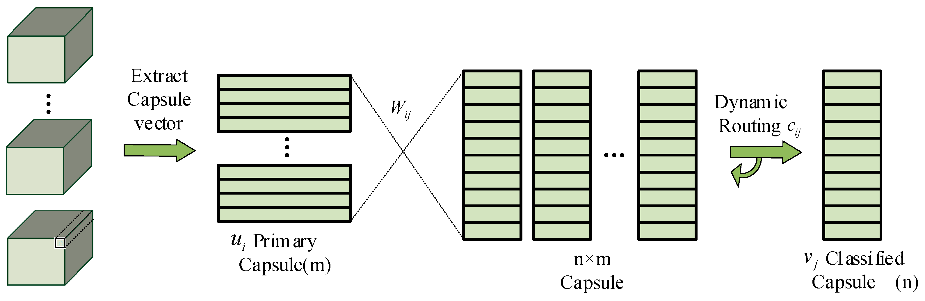
The Capsule Network (CapsNet) proposes replacing neurons in a Convolutional Neural Network with capsules to preserve detailed pose information and spatial hierarchical relationships between objects [12,13,14]. A capsule, in this network, refers to a small group of neurons that can identify a specific object in a defined region. The output of a capsule is a vector with a specific length, representing the probability of object existence, and the vector direction records the object’s attitude parameters. If there is any slight change in the object’s position, such as rotation or movement, the capsule would output a vector with the same length but a slightly varied direction.

In recent years, a Capsule Network has been increasingly utilized in image classification and recognition and has shown promising results [15,16,17,18,19]. Shakhnoza, M applied a Capsule Network to fire smoke image recognition, which demonstrated high recognition accuracy and robustness for outdoor camera image classification in the presence of smoke and fire [15]. Wang, W combined a Convolutional Neural Network and Capsule Network to classify gastrointestinal endoscopic images with a classification accuracy of over 85% for multiple datasets [16]. Sreekala, K developed a deep transfer learning model for face recognition using the Capsule Network and utilized a Grey Wolf Optimization (GWO) and Stacked Autoencoder (SAE) model to classify faces in images [18].

In our study of particleboard surface defect recognition, the recognition process of the defect type is greatly interfered with by the special characteristic of the surface texture of the board. To address this, we introduce an improved CBAM attention model into the Capsule Network. The CBAM (Convolutional Block Attention Module) model is a channel space mixed attention model [20,21,22]. It generates attention feature map information in both channel and space dimensions and multiplies the two feature maps with the original input feature map to perform adaptive feature correction and obtain an optimized feature map. By using the CBAM attention model in the particleboard surface defect classification and recognition problem, important feature information is strengthened, unnecessary features are suppressed, and feature optimization is achieved, resulting in improved recognition accuracy with reduced calculation parameters and computing power being saved.

In the particleboard production line, surface defects must be detected, extracted, classified, and identified to assess the degree of damage to the board. Subsequently, the boards that do not meet surface quality requirements must be removed from production. To achieve this objective, we use the CBAM attention model to improve the Capsule Network and use the improved method to identify five common surface defects (bare shavings, oil spots, glue spots, sand lines, and holes) on the production line. The study has two main aspects. Firstly, we propose an algorithm for the Capsule Network based on the improved CBAM attention model, making it more suitable for identifying particleboard surface defect types. Secondly, we conduct recognition experiments using defect samples from the particleboard surface defect dataset and compare the effectiveness of our model with that of other common recognition methods.

2. Materials and Methods

2.1. The Capsule Network

The network structure of the Capsule Network can be divided into two main parts: the primary part and the reconstruction part [23,24]. The primary part comprises convolution layers, convolution capsule layers, and fully connected capsule layers. On the other hand, the reconstruction part decodes the characteristic vector to assist in reconstructing the input image in cooperation with the Capsule Network. The main part structure of the Capsule Network is illustrated in Figure 1.

The Capsule Network has a network structure that includes two convolution layers and a classified capsule layer based on the dynamic routing algorithm, as shown in Figure 1. The first two layers are similar to those of a Convolutional Neural Network. Notably, the feature map output at the second layer is used to construct the capsule vector. In the third layer, each capsule vector serves as the input and output of the dynamic routing algorithm, and each capsule vector has its corresponding weight matrix. The dynamic routing algorithm is applied to transform the capsules. After the third layer of conversion, the capsule vector is represented by two equations: one represents the current data sample, and the other represents the probability of the corresponding category of the input sample.

In the second convolution layer, the primary capsule layer follows a typical Convolution Network structure. However, it differs from traditional Convolutional Neural Networks in that its role is to process the feature map. As shown in Figure 1, the feature map output from the first convolutional layer is presented on the left side of the primary capsule layer. Unlike traditional Convolutional Neural Networks, which stretch multiple feature map matrices and concatenate them into a vector, the Capsule Network groups all the feature maps according to a specified number, as demonstrated in Figure 2. Capsule vectors are extracted by grouping feature maps based on the channel direction, allowing the convolutional kernel to be separated into multiple groups.

The Capsule Network’s dynamic routing capsule layer performs the conversion of capsule vectors using the principle depicted in Figure 3, as mentioned earlier. The dynamic routing algorithm is a crucial component of the Capsule Network and not only facilitates the implementation of the capsule mechanism but also embodies its ideas. To analyze the principle of the Capsule Network more easily, the lower-level capsule is transformed into a high-level capsule, which serves as the target of the conversion.

Consider $u_i$ as the capsule vector of layer $l$, $v_j$ as the capsule vector of layer $l+1$, which represents the weighted sum of all prediction vectors ${\widehat{u}}_{j|i}$. The change formula can be expressed as:

$${\widehat{u}}_{j|i}=W_{ij}·u_i$$

(1)

where, $W_{ij}$ is the weight matrix that can be learned. Consider $c_{ij}$ is the coupling coefficient corresponding to each prediction vector ${\widehat{u}}_{j|i}$ mapped to $v_i$, which is the weight coefficient. $c_{ij}$ determines the weight required to convert the prediction vector of layer $l$ to the corresponding $v_i$ of layer $l+1$. Since ${\displaystyle \sum {}_j c_{ij}=1}$ can be calculated by dynamic routing algorithm, there are:

$$s_j={\displaystyle \sum _i{c}_{ij}}{\widehat{u}}_{j|i}$$

(2)

Each capsule vector represents the probability of the entity’s occurrence, and the entity can be either an object in the picture or a part of the object. So, the $s_j$ obtained through the calculation of the above formula cannot be used as the vector expression of the high-level capsule $j$. In order to solve this problem, a nonlinear extrusion equation is introduced into the Capsule Network to scale the length of the capsule. By scaling the length of the capsule in this way, the length of the short capsule approaches 0 and the length of the long capsule approaches 1. The length of the capsule represents the probability of the existence of the entity, and its length is between $(0,1)$. The extrusion equation can be expressed as:

$$v_j=\frac{{\Vert s_j\Vert }^2}{1+{\Vert s_j\Vert }^2}\cdot \frac{s_j}{\Vert s_j\Vert }$$

(3)

According to Formulas (2) and (3), we can know how to calculate the prediction vector of $u_i$ to obtain the vector $v_i$ of high-level capsules. In this process, the coupling coefficient $c_{ij}$ is the amount that determines that $u_i$ is “routed” to $v_i$. When the similarity between $u_i$ and $v_i$ is high, the contribution of $u_i$ to $v_i$ is greater, and the value of $c_{ij}$ is greater. Similarly, when the similarity between $u_i$ and $v_i$ is low, the value of $c_{ij}$ is smaller. In the above dynamic routing process, $c_{ij}$ is not calculated by gradient training in a Convolutional Neural Network, but by an iterative process:

$$c_{ij}=\frac{\exp (b_{ij})}{{\displaystyle \sum {}_k\exp (b_{ik})}}$$

(4)

where, $b_{ij}$ is the logarithmic prior probability of the coupling relationship between $u_i$ and $v_j$, and $k$ is the number of iterations. The iterative process described in Formula (4) is the process of dynamic routing, which is the core part of the Capsule Network. Before the first iteration calculation, the initial value of $b_{ij}$ is 0, and the update process can be expressed as:

$$b_{ij}=b_{ij}+{\widehat{u}}_{j|i}·v_j$$

(5)

According to the above principles, the calculation process of dynamic routing can be summarized as follows:

• Calculate the predictive value ${\widehat{u}}_{j|i}$ of $u_i$ from Formula (1), and initialize $b_{ij}$ to 0;
• The coupling coefficient $c_{ij}$ is calculated from Formula (4) and substituted into Formulas (2) and (3) to obtain the intermediate value $s_j$ and the vector $v_j$ of the upper capsule;
• Update $b_{ij}$ by Formula (5);
• Judge whether the iteration is completed. If it is not completed, repeat steps 1–3. If it is completed, output $v_j$.

Dynamic routing routes the original capsule to the category capsule through the above process. The length of the category capsule describes the probability of the existence of the represented category. The final classification category of the image is the category corresponding to the longest capsule. To make the capsules representing the image category as long as possible, a margin loss function is introduced in the Capsule Network. For the category capsule $v_k$, the loss function can be described as:

$$L_k=T_k\max {\left(0,m^{+}-\Vert v_k\Vert \right)}^2+\lambda \left(1-T_k\right)\max {\left(0,\Vert v_k\Vert -m^{-}\right)}^2$$

(6)

where $m^{+}$ and $m^{-}$ are the capsule length thresholds. $\lambda$ is the loss adjustment parameter. $T_k$ is the category parameter. If the image belongs to category $k$, then $T_k=1$, otherwise $T_k=0$. Calculate the loss function values for all categories of capsules, and the sum of which is the loss value for the Capsule Network.

The reconstruction part of the Capsule Network is used to decode the category capsule and reconstruct the image. The reconstructed image and the input image use the sum of pixel differences squared as the image reconstruction loss value $L_I$. The total loss of the reconstruction part of the Capsule Network can be expressed as:

$$L={\displaystyle \sum _k{L}_k+\mu L_I}$$

(7)

where $\mu$ is the reconstruction adjustment parameter. Based on the resulting loss $L$, the training of the Capsule Network can be realized.

2.2. Capsule Network Based on Improved CBAM Attention Model (CBAM-CN)

The basic structural model of CBAM is shown in Figure 4.

For any input feature map $X\in R^{C\times H\times W}$, the feature map obtained after passing the channel attention module is considered as $X^{\prime }$. The feature map obtained after passing the spatial attention module is considered as $X^{″}$, then:

$$X^{\prime }=M_C\left(X\right)\otimes X$$

(8)

$$X^{″}=M_S\left(X^{\prime }\right)\otimes X^{\prime }$$

(9)

where, $M_C$ represent the calculation equations of the channel attention module, and $M_S$ represent the spatial attention module.

In the problem of the board surface defect recognition, due to the limited number of image samples available for training, the training results are prone to overfitting. A good classification effect can be obtained for the test set, but the accuracy in the actual detection is very low. To solve this problem, we introduce a GMLP based on a Gaussian error linear unit, and construct a new attention model of an anti-overfitting channel.

To calculate channel features more efficiently, the channel attention model needs to compress the spatial dimensions of the input features. First, the input feature graph is passed through the parallel maximum pooling layer and the average pooling layer to obtain the maximum pooling feature $F_{\max }^C$ and the average pooling feature $F_{avg}^C$. Then, input the two features to GMLP, and the hidden layer output $H_0$ can be expressed as:

$$H_0=f_{GELU}(X{W}_h+b_h)$$

(10)

where, $W_h$ is the hidden layer weight, $b_h$ is the hidden layer threshold, and $f_{GELU}$ is the Gaussian Error Linear Unit activation equation (GELU). It can be described as follows:

$$f_{GELU}(x)=xP(X\le x)=\frac{x}{2}\left[1+e_{rf}\left(\frac{x}{\sqrt{2}}\right)\right]$$

(11)

where $e_{rf}$ can be expressed as:

$$e_{rf}(x)=\frac{1}{\sqrt{\pi }}{\displaystyle {\int }_{-x}^x{e}^{-t^2}dt}=\frac{2}{\sqrt{\pi }}{\displaystyle {\int }_0^x{e}^{-t^2}dt}$$

(12)

Formula (11) can be approximately described as:

$$f_{GELU}(x)=\frac{x}{2}\left\{1+\tanh \left[\sqrt{\frac{2}{\pi }}\left(x+0.045x^3\right)\right]\right\}$$

(13)

It can be seen from Equation (13) that the multilayer perceptron model using the GELU introduces random regularization while maintaining the nonlinear mapping ability, which can better avoid the generation of the overfitting phenomenon and the disappearance of the gradient. In order to further accelerate the convergence speed of the hidden layers and suppress the gradient disappearance problem in the back-propagation process, each hidden layer is batch normalized, and the process can be expressed as:

$$H_n=f_{BN}\left(H_0\right)=\frac{\gamma \left(H_0-\mu \right)}{\sqrt{{\sigma }^2+\epsilon }}+\beta$$

(14)

where, $f_{BN}$ is the batch normalization equation, $\gamma$ is the scale factor, and $\beta$ is the translation factor.

In order to prevent overfitting, the output characteristics of the hidden layer after batch normalization are randomly deleted by using the Dropout equation, and the final output characteristics of the hidden layer are as follows:

$$H=dropout(H_n)=\{\begin{array}{c}0\hspace{1em},\hspace{1em}r<p\\ \frac{H_n}{(1-p)},\hspace{1em}r\ge p\end{array}$$

(15)

where, $r$ is a random value, of which the value range is $[0,1)$, and $p$ is the dropout coefficient.

The output feature $O$ is obtained by passing the hidden layer output feature $H$. $O$ can be expressed as:

$$O=f_S(H{W}_O+b_O)$$

(16)

where, $W_O$ is the hidden layer weight, $b_O$ is the hidden layer threshold, and $f_S$ is the Sigmoid equation.

To sum up, the output characteristics of the channel attention model can be expressed as:

$$M_C(F)=f_S(F_{\max }^{CH}+F_{avg}^{CH})$$

(17)

where, $F_{\max }^{CH}$ is the hidden layer output feature of the maximum pooling feature $F_{\max }^C$, and $F_{avg}^{CH}$ is the hidden layer output feature of the average pooling feature $F_{avg}^C$. $M_C\in R^{C/r\times 1\times 1}$, and $r$ is the dimension reduction coefficient. The basic structure of the anti-overfitting channel attention model is shown in Figure 5.

After obtaining the channel attention feature $M_C$, the CBAM model continues to calculate the spatial attention feature $M_S$. Average pooling and maximum pooling are performed in the channel dimension to obtain the maximum pooling feature $F_{\max }^S$ and the average pooling feature $F_{avg}^S$. The two are superposed and the dimension is reduced by convolution. In the same way as the channel attention model, the final spatial attention feature map can be obtained after using the Sigmoid equation. $M_S$ can be expressed as:

$$M_S(F)=f_S(f(F_{\max }^S,F_{avg}^S))$$

(18)

where, $F_{\max }^S\in R^{1\times H\times W}$, $F_{avg}^S\in R^{1\times H\times W}$, and $M_S(F)=R^{H,W}$. The basic structure of the spatial attention model is shown in Figure 6.

In summary, the improved CBAM attention model is applied to the convolution layer of the Capsule Network, resulting in reduced interference from the particleboard surface textures and improved recognition accuracy through optimized feature maps. Additionally, the improved Capsule Network model has strong anti-overfitting characteristics due to the adoption of the GELU and the addition of the Dropout layer, which can be more suitable for feature recognition with limited sample sizes. The improved model has good applicability to the problem of particleboard surface defect recognition that this article focuses on.

2.3. Experiment Equipment

The research system comprises an image acquisition system and a detection and recognition system. The image acquisition system should capture particleboard surface images clearly, facilitate further processing by the software environment, and transmit data quickly to the computer software system to ensure the overall detection efficiency of the system. The system should also be economically durable and offer good technical support, taking into account the practicality of the production line.

The image acquisition system in this study meets the aforementioned requirements by selecting the GigE color industrial camera model DFK 23GP031 from the imaging source with an acquisition rate of 15 fps. The camera is equipped with an ON Semiconductor CMOS sensor (MT9P031) that ensures high-quality images while also reducing equipment cost. Additionally, the camera uses a surface scanning mode which enables a quicker collection of the particleboard surface image in the field of vision compared to line-scanning cameras. This ensures real-time detection at the image acquisition level while maintaining high definition.

The image acquisition system used in this study employs two industrial cameras positioned side by side, as depicted in Figure 7. By adopting a dual-camera parallel acquisition mode, the system can cover the entire surface of the particleboard, ensuring a comprehensive acquisition range. Moreover, using two cameras enhances the accuracy of the acquisition, which contributes to the precision and reliability of the recognition and analysis of particleboard surface defect images.

The detection and identification system comprises computer hardware and internal software. The computer hardware system employed in this research includes Microsoft Windows 10 (64-bit), Inter Xeon Silver 4216 CPU, RAM Tesla V100 GPU, 512 GB memory, and 16GB video memory. IC Capture 2.4 serves as the display software of the camera in the image acquisition system, while the deep learning framework used in the experiment is PyTorch. The programming language used is Python 3.7, and the programming environment is PyCharm 20.1.3.

2.4. Sample Acquisition

At the initial stage, over 2000 particleboard surface images with varying types and degrees of surface defects were collected. Parts of the collected particleboard surface images are shown in Figure 8.

The constructed dataset of the particleboard surface defect images has significant application value in verifying the overall effectiveness of the algorithm, as well as the universality and scope of the real reaction algorithm in the process of simulation experiments. Therefore, it is important that the images in the dataset are typical, inclusive, and authentic. To achieve this, the collected images are further screened, sorted, and classified. Atypical images with incomplete defects, blurred images, excessive interference, and other issues are removed, resulting in a set of 2000 standardized images, each sized $120\times 120$ pixels. The number and percentage of images of each defect type included in the dataset are shown in

Table 1. Statistical data of the number and percentage of images of defect types.

Category	Number	Percentage
Shavings	895	44.73
Sand grain	292	14.62
Hole	196	9.80
Glue spot	167	8.37
Oil stain	450	22.48

.

In this study, we collected particleboard surface defect images that encompassed five different types of surface defects: bare particles, sand grains, oil stains, dust stains, and holes. The percentage of frames containing each type of defect in the total sample size of the dataset simulates the frequency difference of these defects in the actual production line. By utilizing these image samples as research objects, we can conduct simulation experiments to ensure the reliability of data analysis and the effectiveness of the results obtained in this article.

3. Results

The sample set of defect features to be tested is divided into a training set and a test set in a 7:3 proportion. The training set comprises 1400 defect feature maps, while the test set contains 600 defect feature maps.

Common classification recognition methods such as an AP Clustering algorithm, SOM Neural Network, Capsule Network (CapsNet), Fast Capsule Network (Fast CapsNet), and the proposed CBAM-Capsule Network (CBAM CapsNet) were selected to identify and compare the types of surface defects. The size of the sliding pane in the AP clustering algorithm is $40\times 40$, and the reference threshold is $P=20$. The SOM Neural Network takes the number of competing layer nodes as 200. CapsNet, Fast CapsNet, and CBAM-CN employ the loss function shown in Formula (6), wherein the loss regulation parameter $\lambda =0.5$, the capsule length threshold $m^{+}=0.9$, $m^{-}=0.1$, and the reconstruction loss as shown in Formula (7), where the reconstruction regulation parameter $\mu =0.05$.

Table 2. Training parameter settings.

Parameter	Value
Initial learning rate	0.01
Momentum	0.99
Weight decay rate	0.001
Epoch	100
Batch size	10

show the other training parameter settings.

Each recognition algorithm is utilized to conduct recognition experiments on the five types of surface defect images. The accuracy rates and F1 score evaluation index results obtained from the recognition experiments on the training set and test set are presented in

Table 3. Classification results of feature images in the training set.

Experimental Methods	Accuracy	F1-Score
AP	0.9158	0.9153
SOM	0.9315	0.9316
CapsNet	0.9629	0.9625
Fast CapsNet	0.9543	0.9542
CBAM-CN ($p=1$)	0.9853	0.9851
CBAM-CN ($p=0.5$)	0.9861	0.9862

and

Table 4. Classification results of feature images in the test set.

Experimental Methods	Accuracy	F1-Score
AP	0.8315	0.8323
SOM	0.8294	0.8312
CapsNet	0.8536	0.8532
Fast CapsNet	0.9025	0.9029
CBAM-CN ($p=1$)	0.9459	0.9453
CBAM-CN ($p=0.5$)	0.9560	0.9556

.

The data show that the CBAM-CN achieves a higher classification accuracy and F1 score than other algorithms in both the training and test sets when recognizing particleboard surface defect feature images with small sample sizes. This indicates that the CBAM-CN proposed in this paper is effective in eliminating background texture interference and improving classification accuracy. Moreover, by comparing the recognition accuracy of the CBAM-CN at dropout probabilities of 0.5 and 1, it is observed that the introduction of a dropout layer into the improved CBAM attention model results in a relatively small gap between the test set and the training set. These results suggest that the CBAM-CN with a dropout layer can better alleviate overfitting problems caused by small sample sizes.

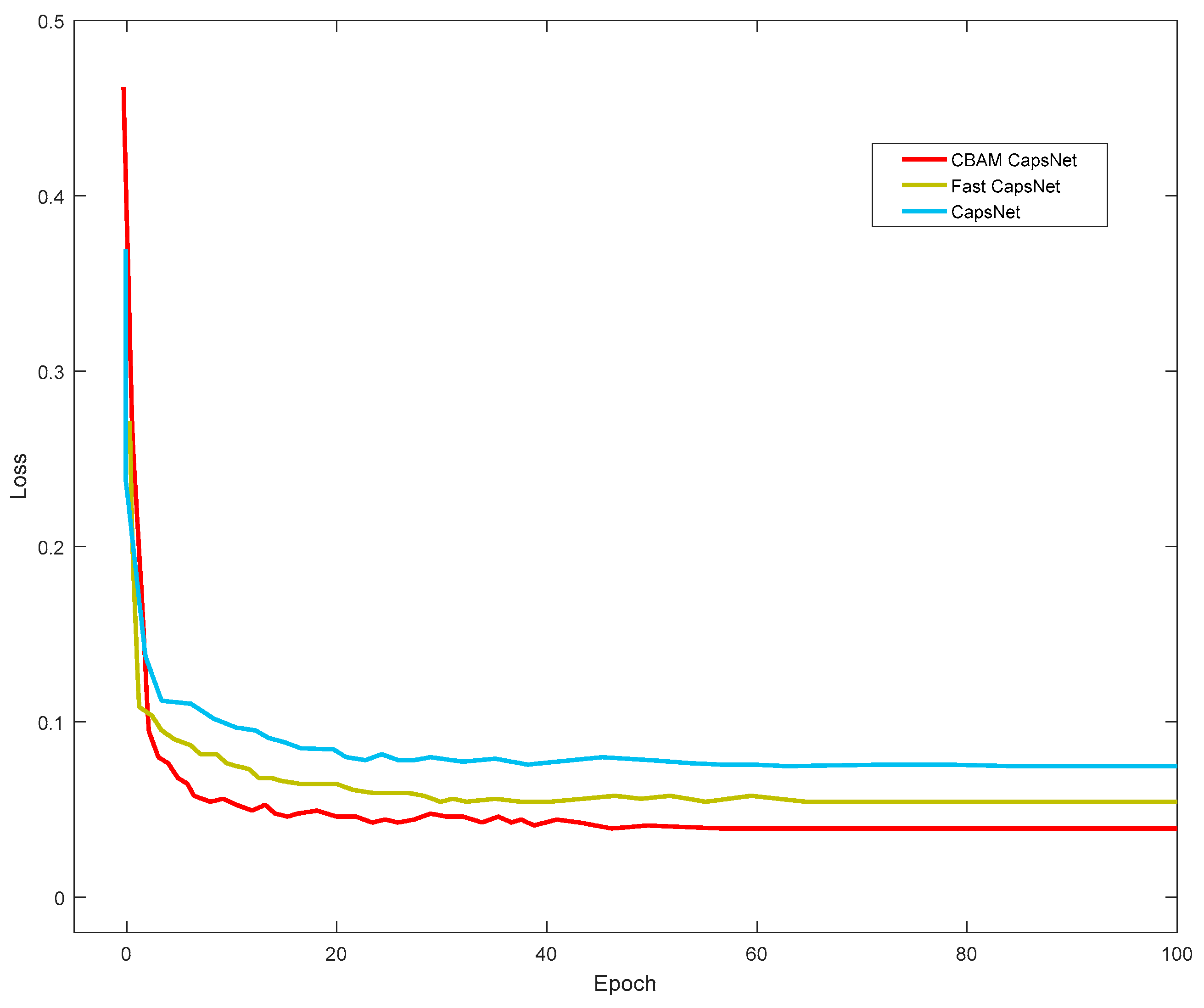
To verify the effectiveness of the CBAM-CN on the particleboard surface defect image sample set, we analyzed the relationship between recognition accuracy, loss rate, and epochs for CapsNet, Fast CapsNet, and the CBAM-CN. The corresponding curves are presented in Figure 9 and Figure 10.

The graph above demonstrates that the CBAM-CN achieves a stable training effect at 40 epochs, while the curves of CapsNet and Fast CapsNet tend to stabilize at 60 epochs. This indicates that the CBAM-CN can optimize the feature graph and improve the training efficiency of the capsule network model. Moreover, it is evident from the curves that the CBAM-CN has higher recognition accuracy and lower loss rate when the training curve tends to be stable, indicating that it can achieve a stable and accurate recognition effect in identifying surface defects of particleboard under the same epoch conditions.

In general, image recognition problems require a large number of training samples for Convolutional Neural Networks to achieve optimal performance. However, in the case of particleboard surface defect recognition, the number of available samples is limited. Therefore, we compare and analyze the recognition accuracy and loss rate of the AP Clustering algorithm, SOM Neural Network, and the CBAM-CN, with varying sample sizes. The resulting curves are shown in Figure 11 and Figure 12. To compare the effects of these recognition algorithms on the problem of overfitting, we include the recognition results of the training set as a comparison in Figure 12. The solid line represents the experimental data of the test set, while the dotted line represents the experimental data of the training set.

The curves in Figure 11 and Figure 12 reveal that when the sample size is small, the training performance of the AP Clustering algorithm and SOM Neural Network will be greatly affected, and a satisfactory recognition effect cannot be achieved. In contrast, the CBAM-CN can achieve an accuracy rate of nearly 85% and a loss rate of less than 15% with just 100 training set samples. When the training set of samples is more than 500, the CBAM-CN can maintain an accuracy rate of more than 90% and a loss rate of less than 5%. On the other hand, other neural network models require over 1000 training samples to attain an accuracy rate of more than 90%. Moreover, under the same number of training samples, the loss rate is also higher than the CBAM-CN.

It is evident from Figure 12 that when the number of samples is small, there is a significant difference between the recognition loss rate of the test set and the training set for the AP Clustering algorithm and SOM Neural Network, indicating the presence of an overfitting problem. However, the two experimental data curves of the CBAM-CN are similar, and it can maintain a low loss rate for the test set even when the number of training samples is small. This result highlights that the CBAM-CN can effectively address the overfitting problem caused by the insufficient number of training samples.

4. Discussion

According to the experimental results and analysis presented above, the CBAM-CN proposed in this article outperforms other effective recognition methods in terms of faster training efficiency and stability for the recognition of particleboard surface defects. Additionally, with a small number of samples in the training set, the CBAM-CN can effectively suppress overfitting and maintain high recognition accuracy. These results also indicate that the CBAM-CN requires fewer training samples to achieve satisfactory recognition results, thereby meeting the recognition requirements for a greater variety of challenging scenes.

5. Conclusions

In this article, we propose a Capsule Network algorithm based on the improved CBAM attention model (CBAM-CN) to tackle the challenges faced by particleboard surface defect recognition technology, including the interference of background texture and the limited availability of image samples for training. We introduce the GELU-enhanced CBAM attention model into the convolution layer of the Capsule Network to optimize the feature map of the surface defects to be detected, thereby improving the model’s training efficiency and stability. Additionally, we add a Dropout layer to alleviate the overfitting problem caused by the small number of samples in the training set, ensuring that the model is more applicable to small sample classification problems. We compare the CBAM-CN with several common effective image recognition methods, and the experimental results demonstrate its effectiveness.

The proposed method in this paper can be analogously applied to other problems of small sample image classification and background texture interference. Further research can experimentally investigate such problems.

References

1. Lee, S.H.; Lum, W.C.; Boon, J.G.; Kristak, L.; Antov, P.; Pędzik, M.; Rogoziński, T.; Taghiyari, H.R.; Lubis, M.A.R.; Fatriasari, W.; et al. Particleboard from agricultural biomass and recycled wood waste: A review. J. Mater. Res. Technol. 2022, 20, 4630–4658. [Google Scholar] [CrossRef]
2. Yang, C.; Lai, W.; Su, J.; He, W.; Gao, Z. Applied Research on Prediction Methods of Properties of Particleboard Based on Data-Driven Methods. J. Biobased Mater. Bioenergy 2021, 15, 1–9. [Google Scholar] [CrossRef]
3. Honarvar, F.; Varvani-Farahani, A. A review of ultrasonic testing applications in additive manufacturing: Defect evaluation, material characterization, and process control. Ultrasonics 2020, 108, 106227. [Google Scholar] [CrossRef] [PubMed]
4. Plessis, A.; Yadroitsava, I.; Yadroitsev, I. Effects of defects on mechanical properties in metal additive manufacturing: A review focusing on X-ray tomography insights. Mater. Des. 2020, 187, 108385. [Google Scholar] [CrossRef]
5. Yang, J.; Li, S.; Wang, Z.; Dong, H.; Wang, J.; Tang, S. Using Deep Learning to Detect Defects in Manufacturing: A Comprehensive Survey and Current Challenges. Materials 2020, 13, 5755. [Google Scholar] [CrossRef]
6. He, T.; Liu, Y.; Yu, Y.; Zhao, Q.; Hu, Z. Application of deep convolutional neural network on feature extraction and detection of wood defects. Measurement 2020, 152, 107357. [Google Scholar] [CrossRef]
7. Zhang, H.; Wang, Y.; Yu, C. Research on Key Technology of Online Detection for Particleboard. In Proceedings of the 2021 IEEE International Conference on Electronic Technology, Communication and Information (ICETCI), Changchun, China, 27–29 August 2021; pp. 512–515. [Google Scholar]
8. Huang, Y.; Qiu, C.; Wang, X.; Wang, S.; Yuan, K. A Compact Convolutional Neural Network for Surface Defect Inspection. Sensors 2020, 20, 1974. [Google Scholar] [CrossRef]
9. Liu, S.; Jiang, W.; Wu, L.; Wen, H.; Liu, M.; Wang, Y. Real-Time Classification of Rubber Wood Boards Using an SSR-Based CNN. IEEE Trans. Instrum. Meas. 2020, 69, 8725–8734. [Google Scholar] [CrossRef]
10. Wu, X.; Qiu, L.; Gu, X.; Long, Z. Deep Learning-Based Generic Automatic Surface Defect Inspection (ASDI) with Pixelwise Segmentation. IEEE Trans. Instrum. Meas. 2021, 70, 1–10. [Google Scholar] [CrossRef]
11. Ding, F.; Zhuang, Z.; Liu, Y.; Jiang, D.; Yan, X.; Wang, Z. Detecting Defects on Solid Wood Panels Based on an Improved SSD Algorithm. Sensors 2020, 20, 5315. [Google Scholar] [CrossRef]
12. Mazzia, V.; Salvetti, F.; Chiaberge, M. Efficient-CapsNet: Capsule network with self-attention routing. Sci. Rep. 2021, 11, 14634. [Google Scholar] [CrossRef]
13. Sun, K.; Yuan, L.; Xu, H.; Wen, X. Deep Tensor Capsule Network. IEEE Access 2020, 8, 96920–96933. [Google Scholar] [CrossRef]
14. Pawan, S.J.; Rajan, J. Capsule networks for image classification: A review. Neurocomputing 2022, 509, 102–120. [Google Scholar] [CrossRef]
15. Shakhnoza, M.; Sabina, U.; Sevara, M.; Cho, Y.-I. Novel Video Surveillance-Based Fire and Smoke Classification Using Attentional Feature Map in Capsule Networks. Sensors 2022, 22, 98. [Google Scholar] [CrossRef]
16. Wang, W.; Yang, X.; Li, X.; Tang, J. Convolutional-capsule network for gastrointestinal endoscopy image classification. Int. J. Intell. Syst. 2022, 37, 5796–5815. [Google Scholar] [CrossRef]
17. Li, D.; Zhang, M.; Kang, T.; Li, B.; Xiang, H.; Wang, K.; Pei, Z.; Tang, X.; Wang, P. Fault diagnosis of rotating machinery based on dual convolutional-capsule network (DC-CN). Measurement 2022, 187, 110258. [Google Scholar] [CrossRef]
18. Sreekala, K.; Cyril, C.P.D.; Neelakandan, S.; Chandrasekaran, S.; Walia, R.; Martinson, E.O. Capsule Network-Based Deep Transfer Learning Model for Face Recognition. Wirel. Commun. Mob. Comput. 2022, 2022, 2086613. [Google Scholar] [CrossRef]
19. Khanal, J.; Tayara, H.; Zou, Q.; To Chong, K. DeepCap-Kcr: Accurate identification and investigation of protein lysine crotonylation sites based on capsule network. Brief. Bioinform. 2021, 23, bbab492. [Google Scholar] [CrossRef]
20. Lu, E.; Hu, X. Image super-resolution via channel attention and spatial attention. Appl. Intell. 2022, 52, 2260–2268. [Google Scholar] [CrossRef]
21. Ju, A.; Wang, Z. Convolutional block attention module based on visual mechanism for robot image edge detection. EAI Endorsed Trans. Scalable Inf. Syst. 2021, 9, e4. [Google Scholar] [CrossRef]
22. Li, G.; Fang, Q.; Zha, L.; Gao, X.; Zheng, N. HAM: Hybrid attention module in deep convolutional neural networks for image classification. Pattern Recognit. 2022, 129, 108785. [Google Scholar] [CrossRef]
23. Huang, Y. Research on dynamic routing algorithm based on gaussian mixture model. MATEC Web Conf. 2022, 355, 03017. [Google Scholar] [CrossRef]
24. Zhang, Q.; Wu, B.; Sun, Z.; Ye, Y. Gating augmented capsule network for sequential recommendation. Knowl.-Based Syst. 2022, 247, 108817. [Google Scholar] [CrossRef]
Figure 1. The main structure diagram of the Capsule Network.
Forests 14 00822 g001
Figure 2. Calculation principle of the capsule layer.
Forests 14 00822 g002
Figure 3. Schematic diagram of dynamic routing.
Forests 14 00822 g003
Figure 4. Basic structure of CBAM.
Forests 14 00822 g004
Figure 5. Basic structure of the channel attention model.
Forests 14 00822 g005
Figure 6. Basic structure of the spatial attention model.
Forests 14 00822 g006
Figure 7. The image acquisition system: (a) DFK 23GP031industrial camera; (b) image acquisition system architecture.
Forests 14 00822 g007
Figure 8. Part of the sample images contains surface defect features (figure (af) are shavings; (g) is sand grain; (h,i) are holes; (j) is glue spot; (k,l) are oil stains).
Forests 14 00822 g008aForests 14 00822 g008b
Figure 9. The relationship between the accuracy and epochs.
Forests 14 00822 g009
Figure 10. The relationship between the loss and epochs.
Forests 14 00822 g010
Figure 11. The relationship between the accuracy and the number of samples.
Forests 14 00822 g011
Figure 12. The relationship between the loss and the number of samples.
Forests 14 00822 g012