Article

Effects of Topography and Social Position on the Solar Radiation of Individual Trees on a Hillslope in Northwest China

Key Laboratory of Forest Ecology and Environment of National Forestry and Grassland Administration, Liupan Mountains Forest Ecosystems National Positioning Observation and Research Station, Ecology and Nature Conservation Institute, Chinese Academy of Forestry, Beijing 100091, China
*
Author to whom correspondence should be addressed.
Forests 2023, 14(3), 561; https://doi.org/10.3390/f14030561
Submission received: 23 February 2023 / Revised: 9 March 2023 / Accepted: 9 March 2023 / Published: 12 March 2023
(This article belongs to the Special Issue Forest Ecohydrology: From Theory to Practice)

Abstract

:
Solar radiation is a key factor influencing the photosynthesis and transpiration of trees. In mountainous regions, solar radiation income exhibits strong spatial heterogeneity due to topographical variations and the structural complexity of the forest. However, how the solar radiation income of individual trees in different social positions varies with slope position remains unclear. In this study, the daily solar radiation of the horizontal ground (Rh), different slope positions (i.e., at different locations on a hillslope, Rs) and individual trees with different social positions in the forest (Ri) were monitored from May to October in 2020 and 2021. The daily solar radiation income of a single hillslope (Rf) was applied to quantify the Rs response to the slope and aspect (i.e., slope effect) and the shade from the opposite mountain (i.e., shaded terrain effect). Our results showed that the Rf was 27.8% lower than Rh due to the slope effect of the sample slope. In the different slope positions, 2.7%–46.9% of solar radiation was lost due to the shaded terrain effect. A stronger limitation of Rs by the shaded terrain effect was detected on the bottom slope compared to that of the upper slope. The better the social position of an individual tree (i.e., tree dominance (Dom) and the distance between trees (D)), the more solar radiation it received, ranging from 22.4 to 95.3%. The dominant factor contributing to changes in Ri was slope position followed by D and Dom and, finally, Rh. These results provide an important basis for understanding the role of topography and tree social positions in solar radiation income in mountainous regions. Forest management measures should be varied with slope positions in mountainous regions, and forest density (i.e., distance between trees) should be considered as a key factor to optimize the forest functions.

1. Introduction

Solar radiation is one of the main environmental signals affecting plant biology, controlling multiple physiological responses [1,2], such as photosynthesis, transpiration and morphogenesis [3,4], with consequences for tree growth [5,6,7,8], which in turn can have an impact on forest productivity [9]. Solar radiation income often shows a high degree of spatial heterogeneity as a result of complex topographical variations and the spatial structure of trees [7,10,11,12,13,14], especially in mountain forests [15,16]. The accurate assessment of the effect of topography and the vertical and lateral position of trees in the forest (i.e., the niche of a tree in a forest is called social position in plant ecology) [17] on solar radiation income is essential for the measurement of solar radiation in mountain forests. Topography variations (such as slope gradient and aspect and the shadows cast by the surrounding topography) have a direct effect on solar radiation income [10,18,19,20,21]. At present, many studies of solar radiation in mountainous regions often focus on the difference in solar radiation income on various hillslopes [11,12,22]. For example, in the Northern Hemisphere, south-facing slopes generally receive a greater amount of solar radiation [23]. Other studies have focused on topographic shading effects [24,25]. The shaded terrain effect by topography leads to a significant reduction in solar radiation income on hillslopes [16]. However, few studies have considered the differences in solar radiation income at different slope positions on hillslopes and whether the shaded terrain effect is consistent at different slope positions.
The solar radiation income of individual trees within forests on hillslopes is also affected by the tree’s spatial structure (i.e., the spatial structure of the tree in both the vertical and horizontal orientation). The essence of the social position of individual trees can describe the spatial information of trees well, which is influenced by different environmental conditions for each tree (i.e., the relative size and distance between the reference tree and its neighbors) and, hence, individuals generate specific social position features [26,27]. The social position of trees determines the living space and available water and radiation resources. Trees with a dominant social position have a vast living space and plenty of water and radiation resources, causing less competition [17]. The degree of dominance and forest density can be used as a proxy indicator [9,28]. Some studies have suggested that the degree of tree dominance affects its ability to receive solar radiation [29], and dominant trees in a stand receive a greater amount of solar radiation [6,30]. Furthermore, decreasing the forest density increases the fraction of the absorbed solar radiation of trees [28,31,32]. However, in many studies, trees were simply divided into different dominance groups based on their relative height or diameter at breast height (DBH) in the forest [7,33,34,35], without considering the shading effects of the surrounding adjacent trees. Assessments of forest density also did not take into account the effect of the social position of individual trees on solar radiation income.
Forests are mainly located in mountainous regions [36]. The rugged mountainous terrain creates a major obstacle to forest management because of the difficult physical approach by men and machines [12,37]. Therefore, it is difficult to accurately quantify the effects of solar radiation income on mountain forests. In addition, forest management is currently focused on the stand scale, i.e., only the stand density is considered without considering the differences in the social location of trees, resulting in the forest management being invalid or only slightly valid [7,38].
To gain a deeper understanding of the effect of topography and social position on the solar radiation income of individual trees, we hypothesize that: (1) solar radiation income is similar at different slope positions; (2) solar radiation income is greater under a more dominant social position. Hence, we aimed to assess the effects of topography and social position on the solar radiation income in a mountainous region, which can help us understand the character of the solar radiation income of trees, so as to make targeted plans for forest management in mountainous regions.

2. Materials and Methods

2.1. Study Site

The study site was located in the small watershed of Xiangshuihe (XSH), Southern Liupan Mountains (106°12′–106°16′ E, 35°27′–35°33′ N) in Ningxia, Northwest China (Figure 1a). XSH has an elevation range of 2010 to 2942 m and a semi-humid climate, with a mean annual air temperature of 5.8 °C and an annual precipitation of 550.8 mm (1981 to 2010); 70% of precipitation occurs in the growing season from May to October. The soil is dominated by gray cinnamon with a sandy loam texture. XSH is a forested watershed with a forest cover of 82.4%, of which plantations account for 24.4%.
The plantations of larch (Larix principis-rupprechtti) are the main components of the plantations in XSH, accounting for 23.6% of the XSH area. Larix principisrupprechtii is the main tree species used in afforestation in North and Northwest China. Such larch plantations play a very important role in producing timber and ecological services (e.g., soil protection, hydrological regulation and water supply) [39,40]. In larch plantations, the understory shrubs were scattered, covering only approximately 5% of the area. Herbs cover approximately 40% of this area, with the dominant species being Pteridium aquilinum and Carex hancokiana.

2.2. Study Slope and Plots

2.2.1. Study Slope

We selected a representative southeastern slope completely covered by an even-aged pure plantation of Larix principis-rupprechtti. The slope had a horizontal length of 425.1 m (corresponding to a slope length of 460.5 m), with a slope gradient of 22.6° and an elevation range of 2271 to 2480 m. The opposite mountain was the northwest slope with a horizontal length of 1052 m, a slope gradient of 23.5° and an elevation range of 2270 to 2731 m. The horizontal distance between the bottom slope of the opposite mountain and the bottom slope of the sample slope was 82 m (Figure 1b–d).

2.2.2. Study Plots

In 2020, four plots were selected at different slope positions on the sample slope, vertically ranging from 2273 to 2471 m a.s.l. The upper slope (US), middle slope (MS), down slope (DS) and bottom slope (BS) were selected with elevations of 2471 m, 2397 m, 2293 m and 2273 m, respectively (Figure 1). These elevation points contain the whole range of the hillslope and the solar radiation received through these elevations can represent the difference amounts of solar radiation received on the whole slope. Also, since the shading of the opposite mountain was more obvious nearer to the bottom of the slope, measurement points were set up on both the down slope and bottom slope. The location information of the Larix principis-ruprechtii plantation plots on the study slope were shown in Table 1. The stand characters of each plot were shown in Table 2.

2.3. Social Position of Trees in the Forest

The social position of trees can represent the trees’ vertical and lateral position in the forest. The trees in the forest were divided into four social position levels according to tree dominance (Dom) and distance between trees (D), as shown by Equations (1) and (2).
D o m = H i H ¯ H ¯
where Hi (m) is the height of the sample tree i and  H ¯  (m) is the average height of all the nearest neighbor trees around the sample tree [17]. The Dom represents the degree of dominance in the vertical direction of the sample tree from neighboring trees.
The distance among trees (D) is defined as the average horizontal distance between the sample tree and its neighboring trees, using Equation (2):
D i = 1 n j = 1 n D i j
where Dij (m) represents the horizontal distance between the sample tree i and the neighbor tree j. The Di represents the degree of superiority or inferiority in the horizontal direction of the sample tree from neighboring trees.
In order to better describe the differences in the social position of trees within the forest, the sample plots at the down slope (DS) were used as an example to illustrate the characteristics of the social position of trees. There were 91 trees in the down slope plot, with a mean tree height (H) of 19.2 m, a mean diameter at breast height (DBH) of 20.63 cm and a mean crown diameter of 4.5 m (Table 2). All trees in the plot were divided into four social position levels according to tree dominance (Dom) and the distance between trees (Di). The vertical structure characteristics of the four social position levels are shown in Table 3.

2.4. Sample Tree Selection from the down Slope Plot (DS)

In the down slope plot (DS), one to two representative trees from each social position level were selected as sample trees using a stratified random sampling method (i.e., sample trees that can represent the average of this level). Therefore, we selected a total of seven sample trees, and the DBH varied in the range of 15.50 to 25.92 cm, the tree height ranged from 17.2 to 21.8 m and the canopy diameter ranged from 3.5 to 5.2 m (shown in Table 4).

2.5. Solar Radiation Measurement

2.5.1. Solar Radiation Data Conversion

The standard for measuring solar radiation utilizes the units of watts per meter squared (W m−2). However, pyranometers are both costly and limited in their ability to measure the solar radiation of individual trees in the slope field. With a lower cost, smaller size and more flexible installation, light meters measure luminous flux per unit area (illuminance), utilizing the units of lumens per meter squared or lux (lx). An effective conversion factor between watts per meter squared and lux would enable the use of light meters to evaluate the differences in the solar radiation in individual tree levels. Additionally, surveys of the literature have found no definitive and readily available “rule of thumb” conversion standard between solar radiation and illuminance data.
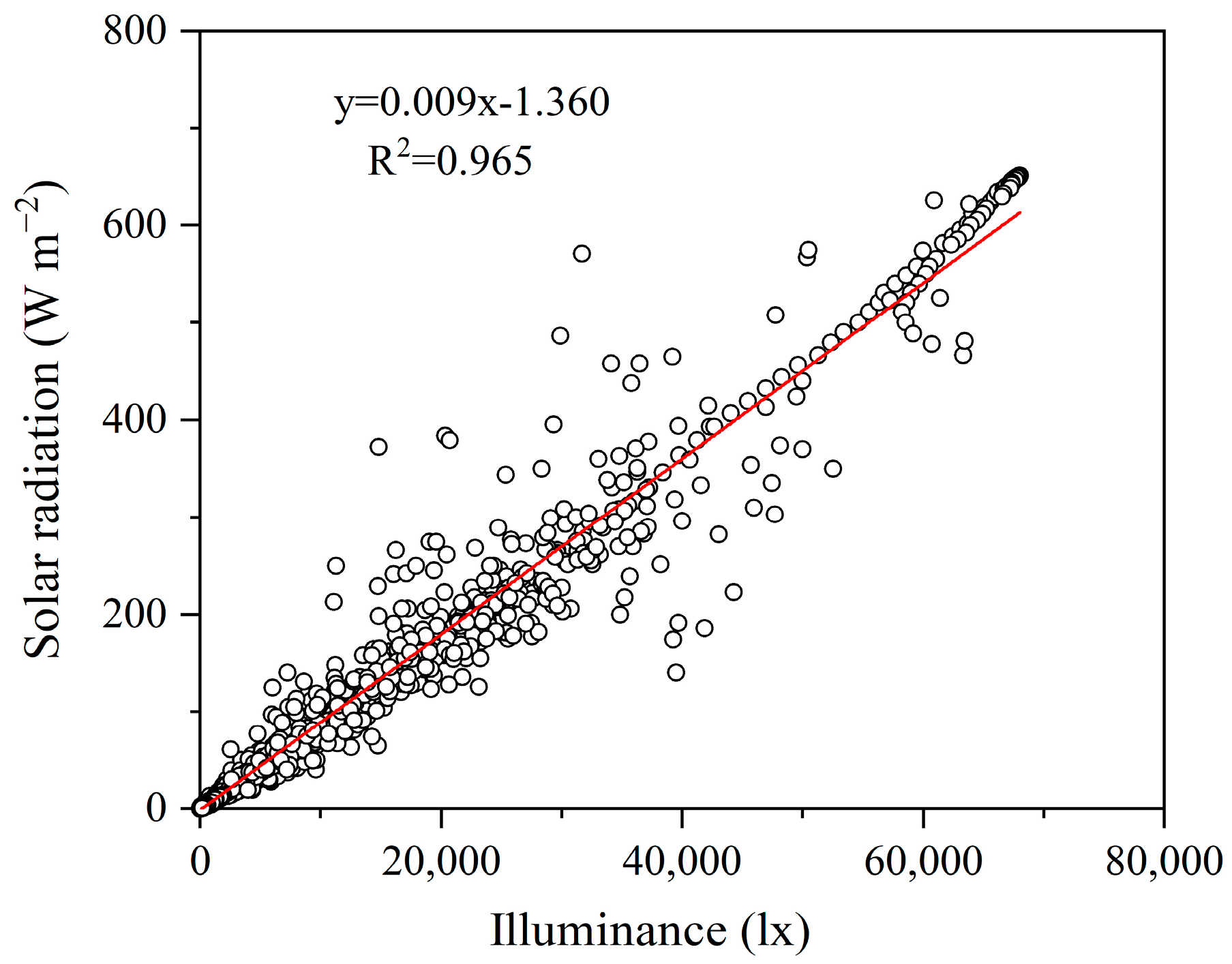
In this study, we converted the illuminance data (lx) into solar radiation data (W m−2) using Equation (3) (Figure 2). This equation was established based on data recorded from a pyranometer in an automatic weather station (Weatherhawk 232; WeatherHawk Inc., Logan, UT, USA) and a light meter (HOBO MX2202; Onset Computer Corp., Bourne, MA, USA). An automatic weather station and a light meter were installed at the same position (i.e., 1.3 m above the ground and the distance between them was 1.0 m) on open and flat horizontal ground approximately 100 m from the sample slope. The data concerning total solar radiation arriving on horizontal ground were collected every 5 min by an automatic weather station (Weatherhawk 232; WeatherHawk Inc., Logan, UT, USA) from May to October in 2020. Radiation data were collected every 5 min by a light meter (HOBO MX2202; Onset Computer Corp., Bourne, MA, USA) from May to October in 2020.
y = 0.009 x 1.360
where y (W m−2) represents the solar radiation and x represents the illuminance (lx).

2.5.2. Solar Radiation of Individual Trees

The daily solar radiation income of individual trees (Ri, MJ m−2 day−1) was measured with a light meter (HOBO MX2202; Onset Computer Corp., Bourne, MA, USA), which was installed at the top of the canopy of each of the seven sample trees. The sensor height of the sample trees is shown in the “Tree Height” column in Table 4. The data concerning the radiation arriving at the top of the canopy were collected every 5 min by the light meter (HOBO MX2202; Onset Computer Corp., Bourne, MA, USA) from July to October 2020 and May to October 2021.

2.5.3. Solar Radiation over the Forest Canopy

The daily solar radiation income over the forest canopy (i.e., outside the forest) on the sample hillslope (Rs, MJ m−2 day−1) was measured in each of the four slope plots (i.e., US, MS, DS and BS) with four light meter loggers (HOBO MX2202; Onset Computer Corp., Bourne, MA, USA) at a height of 1.3 m above the ground. The data concerning the radiation arriving at different slope positions were collected every 5 min by the light meter (HOBO MX2202; Onset Computer Corp., Bourne, MA, USA) from July to October 2020.

2.5.4. Solar Radiation at the Horizontal Ground Measurement

The daily solar radiation income of the horizontal ground (Rh, MJ m−2 day−1) was measured using the pyranometer of an automatic weather station (WeatherHawk 232, WeatherHawk Inc., USA), installed on open and flat horizontal ground approximately 100 m from the sample slope and at a height of 1.3 m above the ground [41]. The data concerning the total solar radiation arriving on horizontal ground were collected every 5 min by an automatic weather station (Weatherhawk 232; WeatherHawk Inc., Logan, UT, USA) from May to October in 2020 and 2021.

2.6. The Calculation of Solar Radiation on a Single Hillslope

The daily solar radiation income of the single hillslope (Rf) was introduced as a reference parameter (that is, the solar radiation of the slope is not affected by the surrounding mountains) and was calculated using the Fu (1958) model [10,42] as follows:
R f = μ sin δ + ϑ cos δ cos ω sin β sin α cos δ sin ω R h
μ = sin φ cos α + cos φ sin α cos β ϑ = cos α cos φ sin φ sin α cos β
where Rf (MJ m−2 day−1) represents the daily solar radiation income of the single hillslope,  β  (°) represents the slope direction (expressed as the azimuth clockwise from north to east) and the slope gradient  α  (°);  δ  (°) is the declination;  ω  (°) is the hour angle; and  φ  (°) is the latitude of the measurement point. The u and v are the composite parameters of the slope gradient  α  (°), the slope direction  β  (°) and the latitude of the measurement point  φ  (°) using Equation (5).

2.7. Relative Contribution of ΔH/Δd, R, Dom and D to Solar Radiation Received by an Individual Tree

The relative independent contributions of ΔHd (the ratio of the height difference to the horizontal distance between the sample point and the top of the opposite mountain, i.e., different slope positions, Δ represents the difference value), Rh, Dom and D to Ri were quantified using the coupled Ri model, and this model was constructed in the Results Section 3.4. The method for determining the relative contribution of each factor to Ri involved a comparison of the difference in the response variable (Ri in this study) between the simulation with only one varying factor (e.g., ΔHd, Rh, Dom and D) and the reference Ri.
The relative independent contributions of ΔHd, Rh, Dom and D to Ri were calculated using Equations (6) and (7) [39]:
C k = Δ R i ( k ) R i ( r e f e r e n c e ) × 100
Δ R i ( k ) = R i ( k ) R i ( r e f e r e n c e )
where Ck (%) is the independent contribution rate of each factor kHd, Rh, Dom and D) to the solar radiation of individual trees (Ri) compared to reference Ri. The reference Ri in this study was calculated using the developed Ri model and the value of ΔHd (0.0, i.e., the sample point has no shaded terrain effect), the long-term means of the Rh (9.32 MJ m−2 day−1, 2013–2021) and the means of Dom (0.001) and D (2.01 m) from all the sample trees (835 trees) on the hillslope. This reference Ri value could represent the long-term mean environmental conditions and social position in this study hillslope. Ri (k) was calculated by inputting the measured value of factor k and the reference values of other factors into the Ri model.

2.8. Statistical Analysis

To clarify how Ri responds to each single factor (Dom and D) and the appropriate function type between Ri and Dom and D, the upper boundary line method [43], which can present the real relation between Ri and a single factor by eliminating the interferences of other factors, was used to determine the RiDom and RiD relation. The upper boundary line was widely used in the establishment of compound models with independent factors as indicators [39].
Statistics were analyzed by the Statistical Product and Service Solutions (SPSS), version 19.0 (IBM Inc., Chicago, IL, USA) and presented as the mean ± standard deviation (SD). The differences in the solar radiation income at the varying slope positions and social positions was analyzed by one-way analysis of variance (ANOVA) with a significance level of p < 0.05, and the letters a and b indicate significant differences [41]. The performance of the model was assessed using the coefficient of determination (R2) [39].

3. Results

3.1. Variation of Solar Radiation at Different Slope Positions

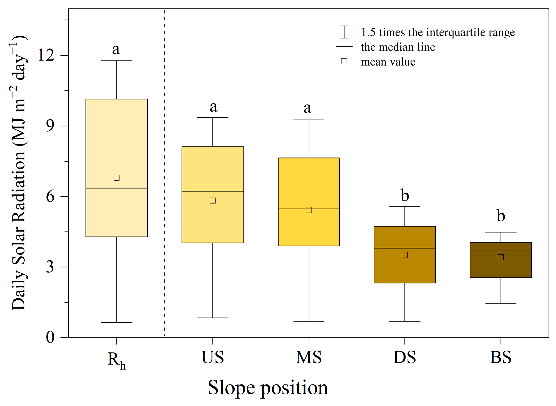
The mean daily solar radiation income at different slope positions (Rs, slope gradient of 27.8°, slope aspect of 135°) was less than that of the horizontal ground (Rh) (Figure 3). The mean Rs at the upper slope (US) and the middle slope (MS) was slightly lower than the Rh (7.03 MJ m−2 day−1) by 1.20 MJ m−2 day−1 and 1.60 MJ m−2 day−1, respectively. However, Rs was even lower on the down slope (DS) and the bottom slope (BS), accounting for only 49.9% and 46.9% of Rh.
Daily solar radiation income of the single hillslope (Rf) was significantly lower than the Rh, accounting for 72.2% of the Rh (Figure 4a). In addition, the Rs was always less than the Rf at the four slope positions by 2.7%–46.9%. The response trend of the Rs to the Rf could be expressed by a saturated logarithmic function, and the threshold of Rs decreased gradually with decreasing slope position (Figure 4b). When Rf was 8.46 MJ m−2 day−1, the difference in solar radiation income between US and MS was not significant, and the corresponding thresholds were 8.23 MJ m−2 day−1 and 8.10 MJ m−2 day−1, respectively. However, the difference in Rs was more pronounced at the DS and BS than at the US, and the corresponding threshold was 5.58 MJ m−2 day−1 and 4.49 MJ m−2 day−1, respectively.
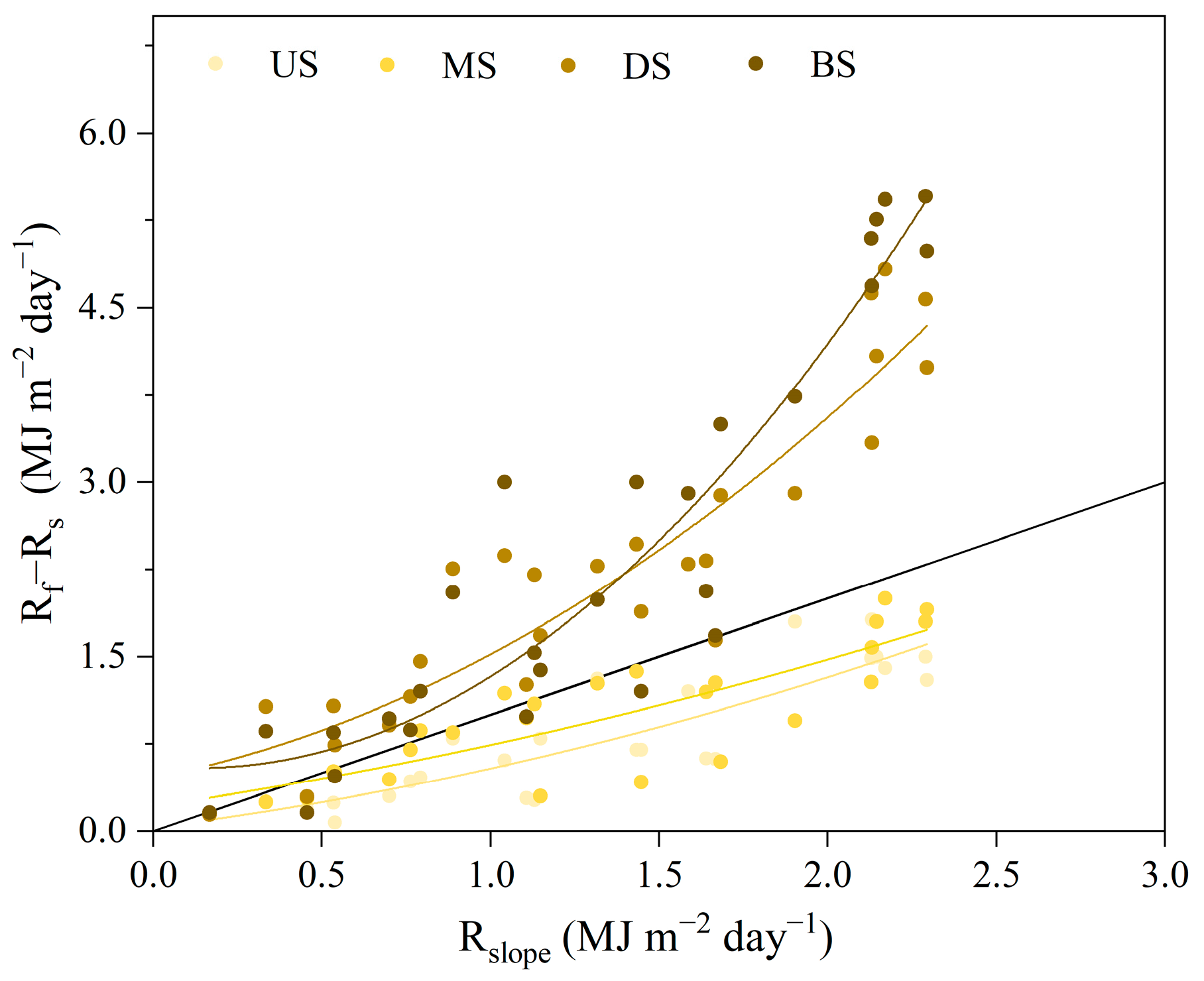
The response trend of RfRs to ΔHd (i.e., the ratio of the height difference to the horizontal distance between the sample point and the top of the opposite mountain) could be expressed by a power function, and RfRs first increased slowly with increasing ΔHd until 0.26 and then increased rapidly (Figure 4c). This indicated that the sample plot was not affected by the shaded terrain effect of the opposite mountain if the RfRs was less than 0.5 MJ m−2 day−1. In addition, the slope effect was always greater than the shaded terrain effect at MS and US, while the shaded terrain effect was more important than the slope effect at DS and BS (Figure 5).

3.2. Effect of Tree Social Position on Its Solar Radiation

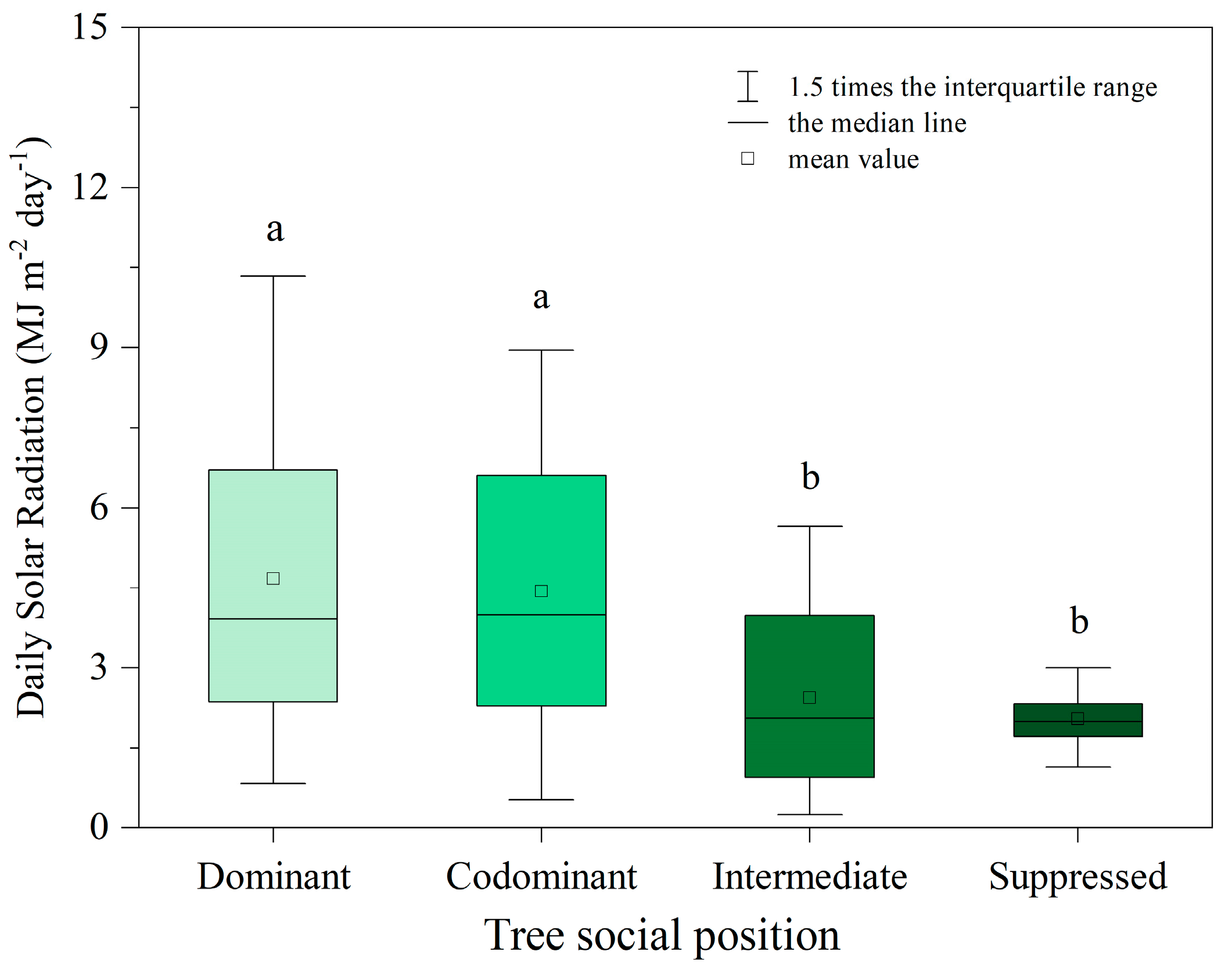
The better the social position of an individual tree, the more solar radiation (Ri) it received (Figure 6). Ri at the dominant level was the largest, followed by Ri at the codominant level and intermediate level and, finally, the suppressed level. The mean Ri of the dominant level (4.82 MJ m−2 day−1) was 1.1 times, 2.0 times and 2.4 times more than the codominant level, the intermediate level and the suppressed level, respectively.
The Ri increased linearly with increasing daily solar radiation income from clearings outside of the forest on the sample slope (Rs) for the four social position levels, ranging from 22.4% to 95.3% (Figure 7a). The relationship between Ri at the dominant level and Rs was more sensitive than that of any other level. For example, the highest coefficient of determination (R2) of the dominant levels was 0.978, which was 1.0, 1.1 and 1.5 times higher than the codominant, intermediate and suppressed levels, respectively. The UBLs in Figure 7b show that Ri gradually increased with the increasing dominance of trees (Dom) following a linear function, namely, Ri = e × Dom + f. Ri first increased rapidly with increasing distance between the trees (D) until 4.5 m and then gradually stabilized around the maximum value as D continued to increase (Figure 7c). The relation between Ri and D could be expressed by a saturated logarithmic function, namely, Ri = g × ln(D) + h.

3.3. The Construction of the Tree Solar Radiation Model and Its Validation

To understand the effect of topography and social position on the solar radiation income of individual trees (Ri), we built a solar radiation model of individual trees, which combined with the results of Section 3.1 and Section 3.2. The Ri model was given as follows:
R i = R h × f t o p o g r a p h y × f s o c i a l   p o s i t i o n
where Ri (MJ m−2 day−1) represents the daily solar radiation income on the sample tree i, Rh (MJ m−2 day−1) represents the daily solar radiation income of the horizontal ground, and f (topography) and f (social position) are the response functions of Ri to topography and social position factors, respectively. The response function of Ri to topography was obtained by the mathematical substitution method. The response functions of Ri to social position (i.e., dominance and distance) were obtained by concatenated multiplication since the solar radiation of individual trees showed a positive correlation with both dominance and the distance between trees (Figure 7b,c).
In addition, combining the methods in Section 2.6, the Ri model can be estimated by Equation (9):
R i = ( a × ( μ sin δ + ϑ cos δ cos ω sin β sin α cos δ sin ω R h b × Δ H Δ d c ) + d ) × e × D o m + f × g × ln D + h
where Ri (MJ m−2 day−1) represents the daily solar radiation income of individual trees, β (°) represents the slope direction (expressed as the azimuth clockwise from north to east) and the slope gradient α (°); δ (°) is the declination; w (°) is the hour angle; and ψ (°) is the latitude of the measurement point. u and v are the composite parameters of the slope gradient α (°), the slope direction β (°) and the latitude of the measurement point ψ (°) using Equation (5). Rh represents the daily solar radiation income of the horizontal ground, ΔHd represents the ratio of the height difference to the horizontal distance between the sample point and the top of the opposite mountain, Dom represents the social position levels of the sample trees, D represents the mean distance between the sample tree and neighboring trees and the a, b, c, d, e, f, g and h values represent the model parameters that need to be determined by the solar radiation data.
All parameters of the Ri model were newly fitted using observed data on the sample slope (slope 27.8°, aspect 135°) from July to October 2020, and the Ri model was further validated using the observed data from May to October 2021, Figure 8. The results indicated that the Ri model could still accurately estimate the varying Ri with a high R2 value (0.83, n = 657). The simulated mean value (4.13 MJ m−2 day−1) was 16.3% greater than the observed mean value (3.55 MJ m−2 day−1). The Ri model of the sample slope was as follows:
R i = ( 0.296 × ( 0.722 R h 107.617 Δ H Δ d 3.963 ) + 0.950 ) × 2.132 D o m + 2.032 × 0.989 ln D 0.426     R 2   =   0.83
In addition, the Ri model accuracy of rain-free days was 0.01 greater than that of the weather-independent model (Figure 8a), with R2 = 0.84, and the accuracy of the Ri model fit was low for rainy days with R2 = 0.61.
R i = ( 2.067 × ( 0.722 R h 107.617 Δ H Δ d 3.963 ) 1.909 ) × 3.786 D o m + 2.667 × 0.789 ln D 0.593     R 2   =   0.84
R i = ( 0.760 × ( 0.722 R h 107.617 Δ H Δ d 3.963 ) + 0.314 ) × 4.414 D o m + 0.825 × 1.078 ln D + 4.582     R 2   =   0.61

3.4. Independent Contributions of ΔH/Δd, Rh, Dom and D to Ri

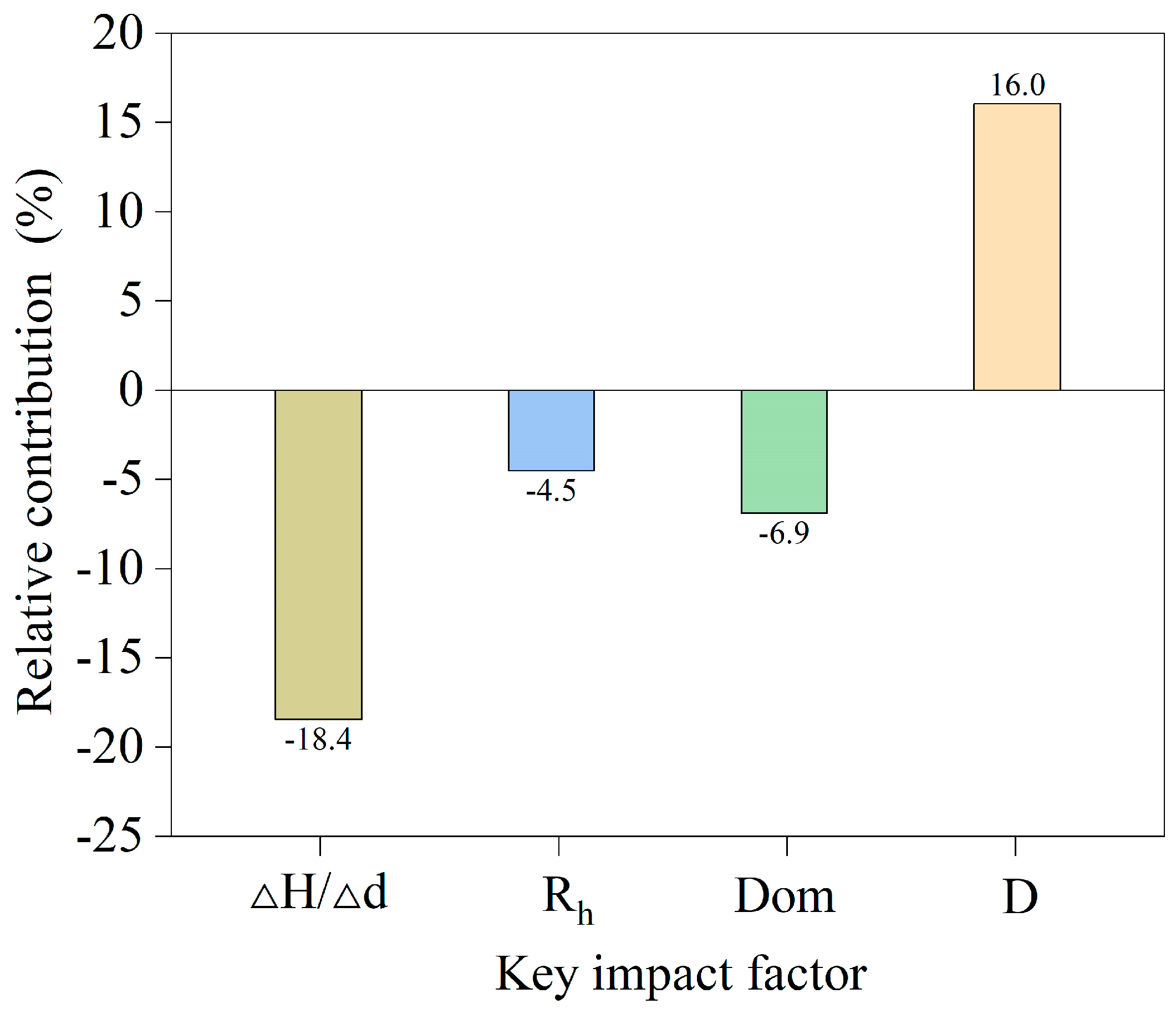
The relatively independent contribution of ΔHd, Rh, Dom and D to Ri compared to the long-term mean of reference Ri is shown in Figure 9. The ΔHd, Rh and Dom exerted slight negative effects on Ri, with contribution rates of −18.4%, −4.5% and −6.9%, respectively, while D had an obviously positive effect on Ri, with a contribution rate of 16.0%. This indicated that variations in slope position had a greater effect on Ri than social position and Rh (i.e., weather variations), and the dominant social position factor affecting the change in Ri was D.
The response of Ri to D exhibited the same trend at different slope positions and different Dom levels, and an obviously higher rate of increase occurred under higher Dom levels (Figure 10). For example, given the ΔHd value of 0.1 and Dom value of 0.3, the effect of D on Ri only gradually decreased when D was greater than 6.0 m, while given the ΔHd value of 0.1 and Dom value of −0.3, Ri stabilized when D was greater than 3.0 m.
There was a significant difference in the effect of D on Ri under different slope positions (i.e., different ΔHd values) (Figure 10). The difference in Ri at different Dom levels gradually decreased as ΔHd values increased, especially after ΔHd > 0.26. For example, given the ΔHd value of 0.1 and Dom value of 0.3, the Ri was above the multi-year means (9.32 MJ m−2 day−1) if the D values were higher than 4.0 m. However, given the ΔHd value of 0.45, the Ri was always less than 9.32 MJ m−2 day−1 regardless of the value of Dom. This indicated that the higher the ΔHd value (i.e., the lower the slope position), the weaker the effect of the social position of trees (both Dom and D).

4. Discussion

4.1. The Role of Topography on Solar Radiation: Slope Effect and Shaded Terrain Effect

In this study, the solar radiation income on the sample slope (slope 27.8°, aspect 135°) was lower than that of the horizontal ground (Figure 3). Similar results were obtained in earlier studies [45,46]. This was mainly because of the slope effect (i.e., slope and aspect) and the shaded terrain effect caused by the opposite mountain [25,47]. Since the slope effect of solar radiation income was the same on a hillslope [42,48], the difference in solar radiation income at different slope positions was mainly caused by different shaded terrain effects. Therefore, we rejected the first hypothesis that the solar radiation income was similar at different slope positions.
The difference in the shaded terrain effect was due to the different blocking effects of topographic features (that is, the distance and elevation difference from the sample slope) [21,49,50]. Our research showed that the shaded terrain effect did not limit solar radiation income on the slope when above the middle slope (i.e., the ratio of the elevation difference to the distance between the sample point and the top of the opposite mountain was satisfied (ΔHd) < 0.26) (Figure 4). This was mainly because the solar radiation income above the mid-slope was not affected by mountain shading due to the difference in height at US and MS, with the opposite mountain being reduced and the distance between the opposite mountain being increased. This was consistent with the result indicating that the forest above the middle slope was not affected by shaded terrain [37].

4.2. The Distance among Trees Was the Dominant Factor for Tree Solar Radiation

The social position of trees (including dominance of trees and distance between trees) was unique for each tree in the forest [14]. Our results suggested that the higher the social position of the individual tree, the more solar radiation it received (Figure 6). This result was completely consistent with our second hypothesis. This was primarily because the trees located in the dominant canopy, which were less shaded by neighboring trees because of a relatively higher tree height [51], could receive more solar radiation [6,7]. Solar radiation income increased as the distance between trees increased (Figure 7), which was consistent with the result indicating that an increase in the distance between trees resulted in greater intakes of solar radiation [52].
However, the contribution of the distance between trees to Ri was more important than that of dominance (Figure 9) because the vertical shading effect among trees weakened as the distance between trees increased [53]. Moreover, the solar radiation income of individual trees increased slowly when the distance between trees was above 4.5 m (Figure 7c), indicating that these trees obtained sufficient solar radiation and the distance between trees was no longer a key factor limiting solar radiation income. This was consistent with the finding that competition among neighbors within 5 m reduced the growth rate due to limited light resources [7,54].

4.3. Applications of the Newly Developed Ri Model

The Ri model developed in this study exhibited a satisfactory performance in estimating the daily solar radiation income of individual trees. The simulated value was 16.3% higher than the observed value since the impacts of leaf variation on solar radiation income were not considered [44]. When simulating only rainy days, the model accuracy was lower at R2 = 0.60 (Figure 8c). This was mostly because on rainy days, cloud cover and ground humidity (changing albedo) in turn affected solar radiation income [55,56]. The developed Ri model couples the effects of topography (including latitude, longitude, elevation, slope and aspect) and the social position of trees (both horizontal distance and vertical dominance), which can easily be obtained in different mountain regions. Foresters could choose suitable measurements according to their actual conditions. For example, horizontal ground solar radiation data can be obtained from ground weather stations, topographic data can be obtained from remote sensing monitoring and the social position of trees can be obtained through field surveys [57].
The Ri model can be used to explain tree growth and thereby regulate forest productivity. For example, a study on this sample slope showed that the cumulative seasonal growth of the down slope plot (1.08 mm) was significantly less than that of the upper slope plot (1.54 mm) because high solar radiation facilitates photosynthesis of organic matter for tree growth and increases air temperature [58]. In addition, on this sample slope, previous transpiration studies focused on the stand scale because of the lack of environmental characteristics of individual trees [37,59,60]. The Ri model in this study accurately predicted the solar radiation received by individual trees, which can be beneficial in explaining the differences in the transpiration of trees. In summary, a series of mountain forest management plans (e.g., thinning) can be made based on the topographic conditions and social position of trees using the developed Ri model to improve the forest structure and alleviate the adverse effects of shade on the solar radiation income of trees.

4.4. Implications for Mountain Forest Management

The solar radiation income of individual trees in forests depended on topographic and social positions. Therefore, different management measures should be adopted for trees at different slope positions and different social positions to promote the receipt of more solar radiation. Our research suggests that the social position of trees (especially the distance between trees) has relevance for mountain forest management.
Different forest management measures should be implemented at different slope positions. When ΔHd > 0.26, the solar radiation income of these slope positions was significantly affected by the shaded terrain effect of the opposite mountain; therefore, the forest density should be reduced by increasing the distance between trees so that residual dominant trees can obtain more solar radiation during the hours of sunshine. For example, given a ΔHd of 0.40 and a Dom of 0.3, the trees can receive a maximum Ri (8.79 MJ m−2 day−1) at a distance between trees of 10.0 m (Figure 10).
However, when ΔHd < 0.26, the shaded terrain effect was almost negligible for the forest, and the shading of adjacent trees was the main factor affecting the solar radiation income of individual trees. The proportion of trees with different social positions can be adjusted by implementing thinning to reduce the light competition among trees. For example, given a ΔHd of 0.10, the daily Ri will be above 9.32 MJ m−2 day−1 when the Dom values are 0.2 and 0.3 with D values of 6.5 m and 4.0 m, respectively (Figure 10).

4.5. Limitations of This Study

The Ri model established in this study can calculate the solar radiation income of trees at any location on the slope. However, due to the experimental conditions, this study only monitored the actual solar radiation income of trees on a sample down slope, so the differences in the solar radiation income of trees in different slope positions could not be verified. Therefore, the reliability of the model estimation will be improved when the model parameters are fitted using the data from more mountainous regions [61].

5. Conclusions

This study focused on the effects of topography and social position on the solar radiation income of individual trees. The slope effect resulted in lower solar radiation income on the hillslope, which was 27.8% lower than that of the horizontal ground. In the different slope positions, 2.7% to 46.9% of solar radiation was lost due to the shaded terrain effect. Solar radiation income above the middle slope was basically unaffected by the shading of the opposite mountain. The more dominant the tree’s social position, the more solar radiation it received, ranging from 22.4% to 95.3%. The dominant factor contributing to the changes in Ri was the distance between trees, and Ri was basically stable when the distance between trees was greater than 4.5 m. The Ri model covered the effect of topography and the social position of individual trees, which explained 83.0% of the observed Ri variation.
These results advanced our understanding of the role of topography and tree social positions of solar radiation income in mountainous regions. Therefore, different forest management strategies should be developed at different slope positions, and the distance between trees should be selected as the main management measure to facilitate the precise adjustment of stand structure design, ensuring that residual trees receive more solar radiation.

Author Contributions

Formal analysis, J.L.; investigation, J.L. and B.L.; writing—original draft, J.L.; writing—review and editing, J.L., P.Y., Y.W. (Yanfang Wan), Y.W. (Yanhui Wang) and Y.Y. All authors have read and agreed to the published version of the manuscript.

Funding

This work was financially supported by the National Natural Science Foundation of China (U21A2005, 42161144008, U20A2085) and the National Key R & D Program of China (2022YFF0801803, 2022YFF1300404).

Data Availability Statement

Not applicable.

Acknowledgments

We thank Liu Hong, Songping Yu, Zhonghui Zhang and Xiaonan Huang for their assistance in the field work.

Conflicts of Interest

The authors declare no conflict of interest.

References

  1. Smith, H. Light Quality, Photoperception, and Plant Strategy. Annu. Rev. Plant Physiol. 1982, 33, 481–518. [Google Scholar] [CrossRef]
  2. Chiang, C.; Olsen, J.E.; Basler, D.; Bånkestad, D.; Hoch, G. Latitude and Weather Influences on Sun Light Quality and the Relationship to Tree Growth. Forests 2019, 10, 610. [Google Scholar] [CrossRef] [Green Version]
  3. Sinoquet, H.; Rakocevic, M.; Varlet-Grancher, C. Comparison of Models for Daily Light Partitioning in Multispecies Canopies. Agric. For. Meteorol. 2000, 101, 251–263. [Google Scholar] [CrossRef]
  4. Wang, H.; Tetzlaff, D.; Dick, J.J.; Soulsby, C. Assessing the Environmental Controls on Scots Pine Transpiration and the Implications for Water Partitioning in a Boreal Headwater Catchment. Agric. For. Meteorol. 2017, 240–241, 58–66. [Google Scholar] [CrossRef] [Green Version]
  5. Lu, Y.; Lei, X.; Hong, L.; Ning, J.; Liu, X.; Meng, J. Demonstrative Application of the Close-to-Nature Forest Management Planning System to Forestry Practice. J. Southwest For. Univ. 2010, 30, 1–6. [Google Scholar]
  6. Binkley, D.; Stape, J.L.; Bauerle, W.L.; Ryan, M.G. Explaining Growth of Individual Trees: Light Interception and Efficiency of Light Use by Eucalyptus at Four Sites in Brazil. For. Ecol. Manag. 2010, 259, 1704–1713. [Google Scholar] [CrossRef]
  7. Binkley, D.; Campoe, O.C.; Gspaltl, M.; Forrester, D.I. Light Absorption and Use Efficiency in Forests: Why Patterns Differ for Trees and Stands. For. Ecol. Manag. 2013, 288, 5–13. [Google Scholar] [CrossRef]
  8. Oogathoo, S.; Houle, D.; Duchesne, L.; Kneeshaw, D. Vapour Pressure Deficit and Solar Radiation Are the Major Drivers of Transpiration of Balsam Fir and Black Spruce Tree Species in Humid Boreal Regions, Even during a Short-Term Drought. Agric. For. Meteorol. 2020, 291, 108063. [Google Scholar] [CrossRef]
  9. Rissanen, K.; Martin-Guay, M.-O.; Riopel-Bouvier, A.-S.; Paquette, A. Light Interception in Experimental Forests Affected by Tree Diversity and Structural Complexity of Dominant Canopy. Agric. For. Meteorol. 2019, 278, 107655. [Google Scholar] [CrossRef]
  10. Fu, B. The total amount of solar radiation on the slope. J. Nanjing Univ. (Nat. Sci.) 1958, 02, 47–82. [Google Scholar]
  11. Prévost, M.; Raymond, P. Effect of Gap Size, Aspect and Slope on Available Light and Soil Temperature after Patch-Selection Cutting in Yellow Birch–Conifer Stands, Quebec, Canada. For. Ecol. Manag. 2012, 274, 210–221. [Google Scholar] [CrossRef]
  12. Baek, S.C.; Park, J.-H.; Na, S.I.; Park, J.-K. Distribution of Solar Radiation Including Slope Effect in South Korea. In Proceedings of the International Society for Optical Engineering; Entekhabi, D., Honda, Y., Sawada, H., Shi, J., Oki, T., Eds.; Kyoto, Japan, 21 November 2012; p. 85242K. Available online: https://www.spiedigitallibrary.org/conference-proceedings-of-spie/8524/1/Distribution-of-solar-radiation-including-slope-effect-in-South-Korea/10.1117/12.977420.short?SSO=1 (accessed on 22 February 2023).
  13. Chen, J.M.; Chen, X.; Ju, W. Effects of Vegetation Heterogeneity and Surface Topography on Spatial Scaling of Net Primary Productivity. Biogeosciences 2013, 10, 4879–4896. [Google Scholar] [CrossRef] [Green Version]
  14. Aakala, T.; Shimatani, K.; Abe, T.; Kubota, Y.; Kuuluvainen, T. Crown Asymmetry in High Latitude Forests: Disentangling the Directional Effects of Tree Competition and Solar Radiation. Oikos 2016, 125, 1035–1043. [Google Scholar] [CrossRef]
  15. Fan, W.; Chen, J.M.; Weimin, J.; Nesbitt, N. Hybrid Geometric Optical–Radiative Transfer Model Suitable for Forests on Slopes. IEEE Trans. Geosci. Remote Sens. 2014, 52, 5579–5586. [Google Scholar] [CrossRef]
  16. Nath, B.; Ni-Meister, W. The Interplay between Canopy Structure and Topography and Its Impacts on Seasonal Variations in Surface Reflectance Patterns in the Boreal Region of Alaska—Implications for Surface Radiation Budget. Remote Sens. 2021, 13, 3108. [Google Scholar] [CrossRef]
  17. Zhang, X. Effects of Social Position and Competition on Tree Transpiration of a Natural Mixed Forest in Chongqing, China. Trees 2019, 33, 719–732. [Google Scholar] [CrossRef]
  18. Garg, H.P.; Datta, G. Fundamentals and Characteristics of Solar Radiation. Renew. Energy 1993, 3, 305–319. [Google Scholar] [CrossRef]
  19. Gracia, M.; Montané, F.; Piqué, J.; Retana, J. Overstory Structure and Topographic Gradients Determining Diversity and Abundance of Understory Shrub Species in Temperate Forests in Central Pyrenees (NE Spain). For. Ecol. Manag. 2007, 242, 391–397. [Google Scholar] [CrossRef]
  20. Liu, B.; Yang, J.; Johnstone, J.F. Understory Vascular Plant Community Assembly in Relation to Time-since-Fire and Environmental Variables in a Chinese Boreal Forest. J. Mt. Sci. 2017, 14, 1317–1328. [Google Scholar] [CrossRef]
  21. Díaz, F.; Montero, H.; Santana, D.; Montero, G.; Rodríguez, E.; Mazorra Aguiar, L.; Oliver, A. Improving Shadows Detection for Solar Radiation Numerical Models. Appl. Math. Comput. 2018, 319, 71–85. [Google Scholar] [CrossRef] [Green Version]
  22. Courbaud, B.; de Coligny, F.; Cordonnier, T. Simulating Radiation Distribution in a Heterogeneous Norway Spruce Forest on a Slope. Agric. For. Meteorol. 2003, 116, 1–18. [Google Scholar] [CrossRef]
  23. Warren, R.J. Mechanisms Driving Understory Evergreen Herb Distributions across Slope Aspects: As Derived from Landscape Position. Plant Ecol. 2008, 198, 297–308. [Google Scholar] [CrossRef]
  24. Zhang, Y.; Chang, X.; Liang, J. Comparison of Different Algorithms for Calculating the Shading Effects of Topography on Solar Irradiance in a Mountainous Area. Environ. Earth Sci. 2017, 76, 295. [Google Scholar] [CrossRef]
  25. Olson, M.; Rupper, S. Impacts of Topographic Shading on Direct Solar Radiation for Valley Glaciers in Complex Topography. Cryosphere 2019, 13, 29–40. [Google Scholar] [CrossRef] [Green Version]
  26. Remeš, J.; Bílek, L.; Novák, J.; Vacek, Z.; Vacek, S.; Putalová, T.; Koubek, L. Diameter Increment of Beech in Relation to Social Position of Trees, Climate Characteristics and Thinning Intensity. J. For. Sci. 2015, 61, 456–464. [Google Scholar] [CrossRef] [Green Version]
  27. Grote, R.; Gessler, A.; Hommel, R.; Poschenrieder, W.; Priesack, E. Importance of Tree Height and Social Position for Drought-Related Stress on Tree Growth and Mortality. Trees 2016, 30, 1467–1482. [Google Scholar] [CrossRef]
  28. Zhang, S.Y.; Ren, H.; Jiang, Z. Wood Density and Wood Shrinkage in Relation to Initial Spacing and Tree Growth in Black Spruce (Picea Mariana). J. Wood Sci. 2021, 67, 30. [Google Scholar] [CrossRef]
  29. Campoe, O.C.; Stape, J.L.; Albaugh, T.J.; Lee Allen, H.; Fox, T.R.; Rubilar, R.; Binkley, D. Fertilization and Irrigation Effects on Tree Level Aboveground Net Primary Production, Light Interception and Light Use Efficiency in a Loblolly Pine Plantation. For. Ecol. Manag. 2013, 288, 43–48. [Google Scholar] [CrossRef]
  30. Gspaltl, M.; Bauerle, W.; Binkley, D.; Sterba, H. Leaf Area and Light Use Efficiency Patterns of Norway Spruce under Different Thinning Regimes and Age Classes. For. Ecol. Manag. 2013, 288, 49–59. [Google Scholar] [CrossRef] [Green Version]
  31. Warren, C.R.; McGrath, J.F.; Adams, M.A. Water Availability and Carbon Isotope Discrimination in Conifers. Oecologia 2001, 127, 476–486. [Google Scholar] [CrossRef] [PubMed]
  32. Hale, S.E. The Effect of Thinning Intensity on the Below-Canopy Light Environment in a Sitka Spruce Plantation. For. Ecol. Manag. 2003, 179, 341–349. [Google Scholar] [CrossRef]
  33. Wan, Y.; Yu, P.; Wang, Y.; Wang, B.; Yu, Y.; Wang, X.; Liu, Z.; Liu, X.; Wang, S.; Xiong, W. The Variation in Water Consumption by Transpiration of Qinghai Spruce among Canopy Layers in the Qilian Mountains, Northwestern China. Forests 2020, 11, 845. [Google Scholar] [CrossRef]
  34. Campoe, O.C.; Stape, J.L.; Nouvellon, Y.; Laclau, J.-P.; Bauerle, W.L.; Binkley, D.; Maire, G.L. Stem Production, Light Absorption and Light Use Efficiency between Dominant and Non-Dominant Trees of Eucalyptus Grandis across a Productivity Gradient in Brazil. For. Ecol. Manag. 2013, 288, 14–20. [Google Scholar] [CrossRef]
  35. Fernández-Tschieder, E.; Binkley, D.; Bauerle, W. Production Ecology and Reverse Growth Dominance in an Old-Growth Ponderosa Pine Forest. For. Ecol. Manag. 2020, 460, 117891. [Google Scholar] [CrossRef]
  36. Li, S. Forest in Mountainous Ecosystem and Its Relationship with Production. Chin. J. Ecol. 1985, 35–38. [Google Scholar]
  37. Tian, A.; Wang, Y.; Webb, A.A.; Liu, Z.; Yu, P.; Xiong, W.; Wang, X. Partitioning the Causes of Spatiotemporal Variation in the Sunny Day Sap Flux Density of a Larch Plantation on a Hillslope in Northwest China. J. Hydrol. 2019, 571, 503–515. [Google Scholar] [CrossRef]
  38. Kübler, D.; Hildebrandt, P.; Günter, S.; Stimm, B.; Weber, M.; Muñoz, J.; Cabrera, O.; Zeilinger, J.; Silva, B.; Mosandl, R. Effects of Silvicultural Treatments and Topography on Individual Tree Growth in a Tropical Mountain Forest in Ecuador. For. Ecol. Manag. 2020, 457, 117726. [Google Scholar] [CrossRef]
  39. Wang, L.; Liu, Z.; Guo, J.; Wang, Y.; Ma, J.; Yu, S.; Yu, P.; Xu, L. Estimate Canopy Transpiration in Larch Plantations via the Interactions among Reference Evapotranspiration, Leaf Area Index, and Soil Moisture. For. Ecol. Manag. 2021, 481, 118749. [Google Scholar] [CrossRef]
  40. Liu, Z.; Wang, Y.; Yu, P.; Xu, L.; Yu, S. Environmental and Canopy Conditions Regulate the Forest Floor Evapotranspiration of Larch Plantations. For. Ecosyst. 2022, 9, 100058. [Google Scholar] [CrossRef]
  41. Liu, Z.; Wang, Y.; Tian, A.; Yu, P.; Xiong, W.; Xu, L.; Wang, Y. Intra-Annual Variation of Stem Radius of Larix Principis-Rupprechtii and Its Response to Environmental Factors in Liupan Mountains of Northwest China. Forests 2017, 8, 382. [Google Scholar] [CrossRef] [Green Version]
  42. Fu, B. The Influence of Slope on the Sunniness. J. Nanjing Univ. (Nat. Sci.) 1958, 02, 23–46. [Google Scholar]
  43. Schmidt, U.; Thöni, H.; Kaupenjohann, M. Using a Boundary Line Approach to Analyze N2O Flux Data from Agricultural Soils. Nutr. Cycl. Agroecosystems 2000, 57, 119–129. [Google Scholar] [CrossRef]
  44. Liu, Z.; Wang, Y.; Tian, A.; Webb, A.A.; Yu, P.; Xiong, W.; Xu, L.; Wang, Y. Modeling the Response of Daily Evapotranspiration and Its Components of a Larch Plantation to the Variation of Weather, Soil Moisture, and Canopy Leaf Area Index. J. Geophys. Res. Atmos. 2018, 123, 7354–7374. [Google Scholar] [CrossRef]
  45. Sun, Z.; Shi, B.; Weng, D. Distribution characteristics of direct solar radiation on mountain slopes in China. Plateau Meteorol. 1990, 9, 371–381. [Google Scholar]
  46. Zeng, Y.; Qiu, X.; Pan, A.; Liu, C. Distributed Modeling of Global Solar Radiation over Rugged Terrain of the Yellow River Basin. Adv. Earth Sci. 2008, 23, 1185–1193. [Google Scholar]
  47. Zhang, S.; Li, X.; She, J. Error Assessment of Grid-based Terrain Shading Algorithms for Solar Radiation Modeling over Complex Terrain. Trans. GIS 2020, 24, 230–252. [Google Scholar] [CrossRef]
  48. Shi, G.; Qiu, X.; Zeng, Y. New Method for Estimating Daily Global Solar Radiation over Sloped Topography in China. Adv. Atmos. Sci. 2018, 35, 285–295. [Google Scholar] [CrossRef]
  49. Aguilar, C.; Herrero, J.; Polo, M.J. Topographic Effects on Solar Radiation Distribution in Mountainous Watersheds and Their Influence on Reference Evapotranspiration Estimates at Watershed Scale. Hydrol. Earth Syst. Sci. 2010, 14, 2479–2494. [Google Scholar] [CrossRef] [Green Version]
  50. Marsh, C.B.; Pomeroy, J.W.; Spiteri, R.J. Implications of Mountain Shading on Calculating Energy for Snowmelt Using Unstructured Triangular Meshes: Implications of Mountain Shading for Snowmelt. Hydrol. Process. 2012, 26, 1767–1778. [Google Scholar] [CrossRef] [Green Version]
  51. Laurans, M.; Hérault, B.; Vieilledent, G.; Vincent, G. Vertical Stratification Reduces Competition for Light in Dense Tropical Forests. For. Ecol. Manag. 2014, 329, 79–88. [Google Scholar] [CrossRef]
  52. Chase, C.W.; Kimsey, M.J.; Shaw, T.M.; Coleman, M.D. The Response of Light, Water, and Nutrient Availability to Pre-Commercial Thinning in Dry Inland Douglas-Fir Forests. For. Ecol. Manag. 2016, 363, 98–109. [Google Scholar] [CrossRef]
  53. Strand, M.; Löfvenius, M.O.; Bergsten, U.; Lundmark, T.; Rosvall, O. Height Growth of Planted Conifer Seedlings in Relation to Solar Radiation and Position in Scots Pine Shelterwood. For. Ecol. Manag. 2006, 224, 258–265. [Google Scholar] [CrossRef]
  54. Chi, X.; Tang, Z.; Xie, Z.; Guo, Q.; Zhang, M.; Ge, J.; Xiong, G.; Fang, J. Effects of Size, Neighbors, and Site Condition on Tree Growth in a Subtropical Evergreen and Deciduous Broad-leaved Mixed Forest, China. Ecol. Evol. 2015, 5, 5149–5161. [Google Scholar] [CrossRef]
  55. Huang, D.; Qian, Y. The effects of the slope irradiance on different weather processes under different model resolutions. Acta Meteorol. Sin. 2008, 01, 90–100. [Google Scholar]
  56. Choosakul, N.; Buddhakala, M.; Barnthip, N.; Muakngam, A.; Banglieng, C. Application of Solar Cells for Daytime Weather Study. Energy Procedia 2011, 9, 171–177. [Google Scholar] [CrossRef] [Green Version]
  57. Hassan-Esfahani, L.; Torres-Rua, A.; Jensen, A.; McKee, M. Assessment of Surface Soil Moisture Using High-Resolution Multi-Spectral Imagery and Artificial Neural Networks. Remote Sens. 2015, 7, 2627–2646. [Google Scholar] [CrossRef] [Green Version]
  58. Ma, J.; Guo, J.; Wang, Y.; Liu, Z.; Gao, D.; Hong, L.; Zhang, Z. Variations in Stem Radii of Larix Principis-Rupprechtii to Environmental Factors at Two Slope Locations in the Liupan Mountains, Northwest China. J. For. Res. 2021, 32, 513–527. [Google Scholar] [CrossRef]
  59. Cao, G. Hydrological Impact and the Slpoe Scale Effect of the Vegetation Structure in the Xiangshuihe Watershed in Liupan Mountains. Ph.D. Thesis, Chinese Academy of Forestry, Beijing, China, 2014. [Google Scholar]
  60. Liu, Z. Spatio-Temporal Variations and Scale Transition of Hydrological Impact of Larix Principis-Ruprechtii Plantation on a Slope of Liupan Mountains, China. Ph.D. Thesis, Chinese Academy of Forestry, Beijing, China, 2018. [Google Scholar]
  61. Sawano, S.; Hotta, N.; Tanaka, N.; Tsuboyama, Y.; Suzuki, M. Development of a Simple Forest Evapotranspiration Model Using a Process-Oriented Model as a Reference to Parameterize Data from a Wide Range of Environmental Conditions. Ecol. Model. 2015, 309–310, 93–109. [Google Scholar] [CrossRef]
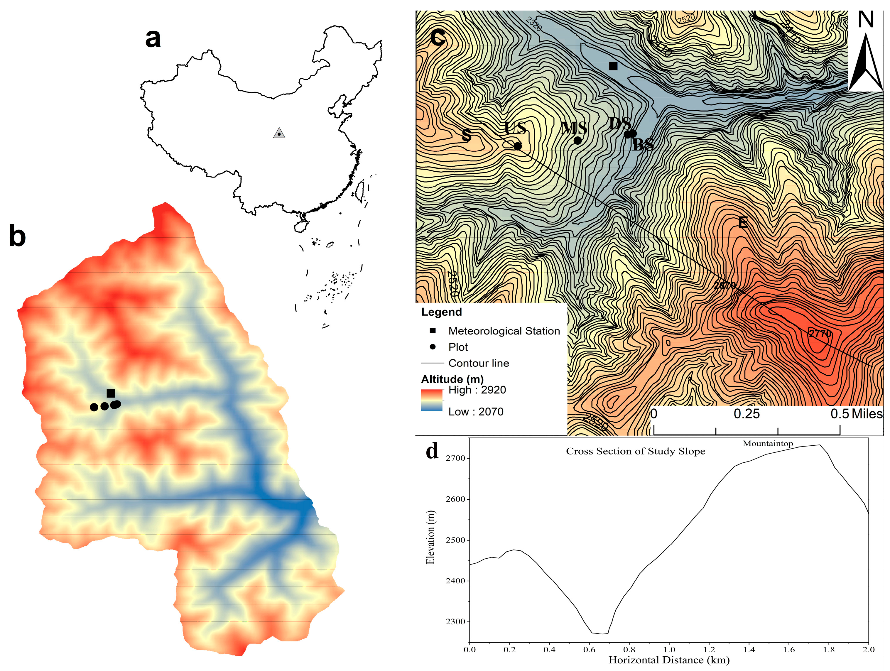
Figure 1. Information about the locations of the study sample plots and sample trees. (a) Location of the Xiangshuihe (XSH) study watershed in NW China. (b) The location of plots (US, MS, DS and BS represent the upper, middle, down and bottom slope) along slope positions on the sample hillslope. (c) The detailed terrain of the study slope and opposite slope. (d) The valley cross-section.
Forests 14 00561 g001
Figure 2. Relationship between solar radiation and illuminance data.
Forests 14 00561 g002
Figure 3. The differences in solar radiation income at various slope positions. (Rh represents the daily solar radiation income of horizontal ground; US represents the upper slope; MS represents the middle slope; DS represents the down slope; BS represents the bottom slope). 1.5 times IQR (interquartile range) was used to determine the anomalous values. Groups marked by different letters significantly differ from each other (i.e., a is significantly greater than b) (p ≤ 0.05).
Forests 14 00561 g003
Figure 4. Effect of topographic change on solar radiation income on the hillslope. (a) The relationship between Rf and Rh. Rh represents the daily solar radiation income of the horizontal ground; Rf represents the daily solar radiation income of the single hillslope. (b) The relationship between Rs and Rf in different slope positions. Rs represents the daily solar radiation income outside the forest on the sample slope. The solid black line in (b) represents Rf = Ri. (c) The relationship between slope position and shade terrain effect. (RfRs) represents the shaded terrain effect of the opposite mountain; ΔHd represents the ratio of the height difference to the horizontal distance between the sample point and the top of the opposite mountain (i.e., the variation of the slope position), the ΔH value represents the elevation difference between the sample point and the opposite mountain top; the Δd value represents the horizontal distance between the sample point and the opposite mountain top; upper slope (US), middle slope (MS), down slope (DS) and bottom slope (BS). The (ΔHd < 0.26) was the threshold indicating that the sample point has no shaded terrain effect, that is, RfRs < 0.5 MJ m−2 day−1.
Forests 14 00561 g004
Figure 5. Comparison of the slope effect and the shaded terrain effect at different slope positions. Rslope represents the slope effect (i.e., RhRf).
Forests 14 00561 g005
Figure 6. The differences in the solar radiation income of individual trees among social position levels in the down slope plot. Groups marked by different letters significantly differ from each other (i.e., a is significantly greater than b) (p ≤ 0.05).
Forests 14 00561 g006
Figure 7. Effect of social positions on the solar radiation income of individual trees. (a) Response of Ri to Rs. (Ri represents the daily solar radiation income of individual trees; Rs represents the daily solar radiation income outside the forest of the sample slope). (b) Response of Ri to Dom (Dom represents the social position levels of the sample trees). (c) Response of Ri to D. (D represents the mean distance between the sample tree and neighboring trees). The upper boundary line (UBL) method [44] was used to determine the response function types of Ri to Dom and D.
Forests 14 00561 g007
Figure 8. Comparison of the observed and simulated Ri values based on Equations (10)–(12) under the different weather conditions. (a) Comparison of the observed and simulated Ri values for all days. (b) Comparison of the observed and simulated Ri values for rain free days. (b) Comparison of the observed and simulated Ri values for all days. (c) Comparison of the observed and simulated Ri values for rainy days.
Forests 14 00561 g008
Figure 9. Relative contribution rate of Rh, Dom and D to the daily solar radiation income of individual trees (Ri) compared to a reference Ri. The reference Ri was modeled by Equation (10) with the long-term means of Rh, the ΔHd value of 0 (Figure 5c) and the mean Dom and D of the 835 sample trees on the hillslope. (ΔHd represents the ratio of the height difference to the horizontal distance between the sample point and the top of the opposite mountain (i.e., the variation of slope position); Rh represents the daily solar radiation income of the horizontal ground; Dom represents the social position levels of sample trees; D represents the mean distance between trees and neighboring trees).
Forests 14 00561 g009
Figure 10. Variation in the simulated Ri with Rh at different Dom and slope position levels by the Ri model (Equation (10)). The value of Rh of 9.32 MJ m−2 day−1 used the long-term mean values from 2013 to 2021. ΔHd represents the ratio of the height difference to the horizontal distance between the sample point and the top of the opposite mountain. ΔHd = 0.26 was the threshold indicating that the sample point had no shaded terrain effect (Figure 4c).
Forests 14 00561 g010
Table 1. The location information of Larix principis-ruprechtii plantation plots on the study slope.
Plot PositionsElevation (m)Slope Gradient (°)Elevation Difference (ΔH)Horizontal Distance (Δd)
Upper slope (US)247126.32591501
Middle slope (MS)239726.83331339
Down slope (DS)229329.04371092
Bottom slope (BS)227334.94571050
The ΔH represents the elevation difference between the sample point and the opposite mountain top; the Δd represents the horizontal distance between the sample point and the opposite mountain top.
Table 2. The stand characteristics of Larix principis-ruprechtii plantation plots on the study slope.
Plot PositionsStand Density (Trees ha−1)Mean Diameter at Breast Height (cm)Mean Tree Height (m)Mean Canopy Diameter (m)
Upper slope (US)85621.8319.44.5
Middle slope (MS)84422.2920.03.7
Down slope (DS) 74220.6319.24.5
Bottom slope (BS) 71121.4019.54.4
Table 3. The vertical structure characteristics of Larix principis-rupprechtii plantation plot in the down slope (DS) (means ± standard deviations).
Tree Social
Position Levels
Number of TreesMean Diameter at Breast Height (cm)Mean Tree Height (m)Mean Canopy Diameter (m)
Dominant 825.30 ± 1.721.8 ± 1.84.9 ± 0.5
Codominant 4021.19 ± 2.219.8 ± 1.44.6 ± 0.4
Intermediate 3119.16 ± 1.918.6 ± 1.74.3 ± 0.6
Suppressed 1215.40 ± 2.517.1 ± 2.33.6 ± 0.5
Table 4. The characteristics of seven sample trees in the down slope plot (DS).
Tree Social
Position Levels
Tree No.Dom
Value
D
Value (m)
Diameter at Breast Height (cm)Tree
Height (m)
Canopy Diameter (m)
Dominant290.124.825.9221.85.2
570.114.524.3421.54.8
Codominant610.013.921.5019.84.4
690.003.321.1119.64.6
Intermediate43−0.043.019.5318.54.2
44−0.042.918.8218.44.0
Suppressed81−0.212.215.5017.23.5
Disclaimer/Publisher’s Note: The statements, opinions and data contained in all publications are solely those of the individual author(s) and contributor(s) and not of MDPI and/or the editor(s). MDPI and/or the editor(s) disclaim responsibility for any injury to people or property resulting from any ideas, methods, instructions or products referred to in the content.