A Multi-Parametric Investigation on Waterlogged Wood Using a Magnetic Resonance Imaging Clinical Scanner

Abstract

In cultural heritage conservation science, moisture content (MC) is an essential factor to determine. At the same time, it is essential to choose non-destructive and non-invasive approaches for more sustainable investigations and make them safe for the environment and the sample. The question addressed in this work concerns the possibility and the opportunity to investigate waterlogged wood by using nuclear magnetic resonance imaging (MRI) clinical scanners to carry out non-destructive volumetric diagnostics. In this study, MRI, the most important non-invasive medical imaging technique for human tissue analysis, was applied to study archaeological waterlogged wood samples. This type of archaeological material has a very high moisture content (400%–800%), thus, it is an ideal investigative subject for MRI which detects water molecules inside matter. By following this methodology, it was possible to obtain information about water content and conservation status through a T₁, T₂, and T₂* weighted image analysis, without any sampling or handling, and the samples were directly scanned in the water where they were stored. Furthermore, it permited processing 3D reconstruction, which could be an innovative tool for the digitalization of marine archaeological collections. In this work, 16 modern species of wood and a waterlogged archaeological wood sample were studied and investigated using a clinical NMR scanner operating at 3T. The results were compared with X-ray computed tomography (CT) images, as they had already been used for dendrochronology. The comparison highlights the similar, different, and complementary information about moisture content and conservation status in an all-in-one methodology obtainable from both MRI and CT techniques.

1. Introduction

Wood is a hygroscopic porous material comprised of cellulose, hemicellulose, lignin, and water, and it has always been used by man [1] due to its extreme versatility and abundance. Fresh wood is composed of 25%–35% lignin, while cellulose and hemicelluloses constitute 65%–75% of the mass, and up to 10% consists of extractives such as pectins, tannins, resins, and oils [2,3,4].

Excavated archaeological wood has a very different structure with respect to fresh wood since it is subjected to various chemical and biological degradation processes [5,6]. It has a very high moisture content (400%–800%) and, in seawater conditions, its entire microstructure is filled with water [6]. Submerged wood decay is accelerated if it is extracted from the water because profound shrinkages and even collapse may occur. For this reason, waterlogged wood remains are usually stored and treated in water [6], proving to be an ideal investigative subject for water-transfer studies.

Furthermore, the development of non-destructive techniques for investigating wood structure and the state of preservation of wooden products without compromising their integrity is highly desirable. In fact, it is not always possible to extract a sample from an analyzed object because most of the ancient artifacts are painted or strongly degraded [7,8,9,10,11,12,13,14] and therefore, it difficult to choose a good sampling area.

These peculiarities make waterlogged wood the ideal material to be investigated by nuclear magnetic resonance (NMR), a widespread medical technology that detects hydrogen atoms inside soft tissues [13,15,16,17,18,19].

In NMR spectroscopy, because of nuclear paramagnetism, macroscopic magnetization (M₀) is generated when hydrogen nuclei spins are immersed in a strong static magnetic field B₀. Then, an electromagnetic field in the radiofrequency (RF) range is used for stimulating the spins to absorb energy. The RF stimulation moves the magnetization M₀ from the direction parallel to B₀ to the direction perpendicular to B₀. When the spins of the hydrogen nuclei are no longer stimulated, they return to their initial state, generating signals that the RF probe receives as electromotive force. The intensity of the acquired NMR signal is proportional to the number of hydrogen spins in the volume investigated (i.e., the spin density) [20,21,22]. The NMR signal decays exponentially in time because of spin-spin and spin-lattice relaxation processes, which are quantified by T₂ and T₁ parameters, respectively.

Magnetic resonance imaging (MRI) is based on NMR spectroscopy, and it is obtained by superimposing time-dependent and controlled magnetic field gradients on the main magnetic field. In this way, MR images are acquired similarly to X-ray computed tomography (CT) scanners [23,24,25,26,27]. However, different from CT images representative of the spatial distribution mapping of the linear attenuation coefficient for X-rays [23,24], the principal sources of the NMR image contrast differences are the spin density and the relaxation times T₁ and T₂ of mobile protons in liquids and macromolecules. The quality of NMR images and their signal-to-noise ratio (SNR) improve in parallel to an increase in the number of mobile protons (water). A high SNR is necessary for enhancing the spatial resolution, which depends on the magnetic field gradients strength (g) used to obtain spatially resolved NMR information [20,21,28].

Currently, although MRI as CT is widely used to observe internal parts of the human body with little harm to the patient, its application to wood science and wooden cultural heritage diagnostics [27,29,30,31,32,33] is still to be developed, but nevertheless is a constantly evolving field.

One of the first works that highlighted the potential of MRI for studying wood was performed by Wang et al. [29] on a sample of cherry wood using a clinical scanner of 0.15 T. Other authors [30,34] have obtained images with an in-plane resolution of about 1 × 1 mm². Interesting results have been obtained in the field of dendrochronology [27,35], forest sciences [32,33,36], materials sciences, and archaeological woods [13,31,37]. Despite the potential usefulness in the physiological and microstructural study of wood, the presence of papers in the literature concerning the application of MRI for the recognition of wood characteristics, wood properties, and their conservation status is still limited [27,31,33,38,39,40,41,42,43]; therefore, MRI remains to be a non-consolidated technique for the above-mentioned purposes. Moreover, in recent years, the development of MRI clinical scanners has been remarkable, allowing us to obtain high-quality images for the investigation of human tissues. In parallel, different types of software dedicated to NMR image analysis and three-dimensional reconstruction of organs and tissues have been developed to optimize medical diagnostics [44]. These types of software allow zooming, manipulation, and rotating an image without losing image quality but highlighting image contrast differences. This allows an accurate inspection of all the different sides of an object and observations with more details.

The aim of this work was to develop and test a non-destructive and non-invasive MRI protocol on clinical scanners, which, potentially, could be useful for the diagnostics of waterlogged wood. Specifically, the purpose was to investigate the conservation state and to identify the wood anatomical features of interest in the field of cultural heritage. Towards this goal, two phantoms made of different wood species (32 in total, both hardwood and softwood), i.e., one water-imbibed phantom and another phantom at environmental humidity (30%), and a waterlogged archeological wood sample were all scanned at 3 T magnetic field. This study shows NMR images obtained on different wood species with an in-plane resolution of 250 × 250 μm². The images show contrast differences being weighted in T₁, T₂, and T₂* parameters. Different wood structures were identified and discussed in relation to NMR image multiparametric contrast. Moreover, proton density, relaxation time maps, and 3D reconstruction are presented together with T₁, T₂, and T₂* measurements of water in each wood species. The correlation of NMR parameters with the density (in kg/m³) of each wood species was carried out considering both imbibed and naturally hydrated wood samples. Finally, a comparison between MRI and CT images obtained on the same wood samples was performed to highlight the complementary and multiple information provided by the MRI investigation.

2. Materials and Methods

2.1. Wood Samples

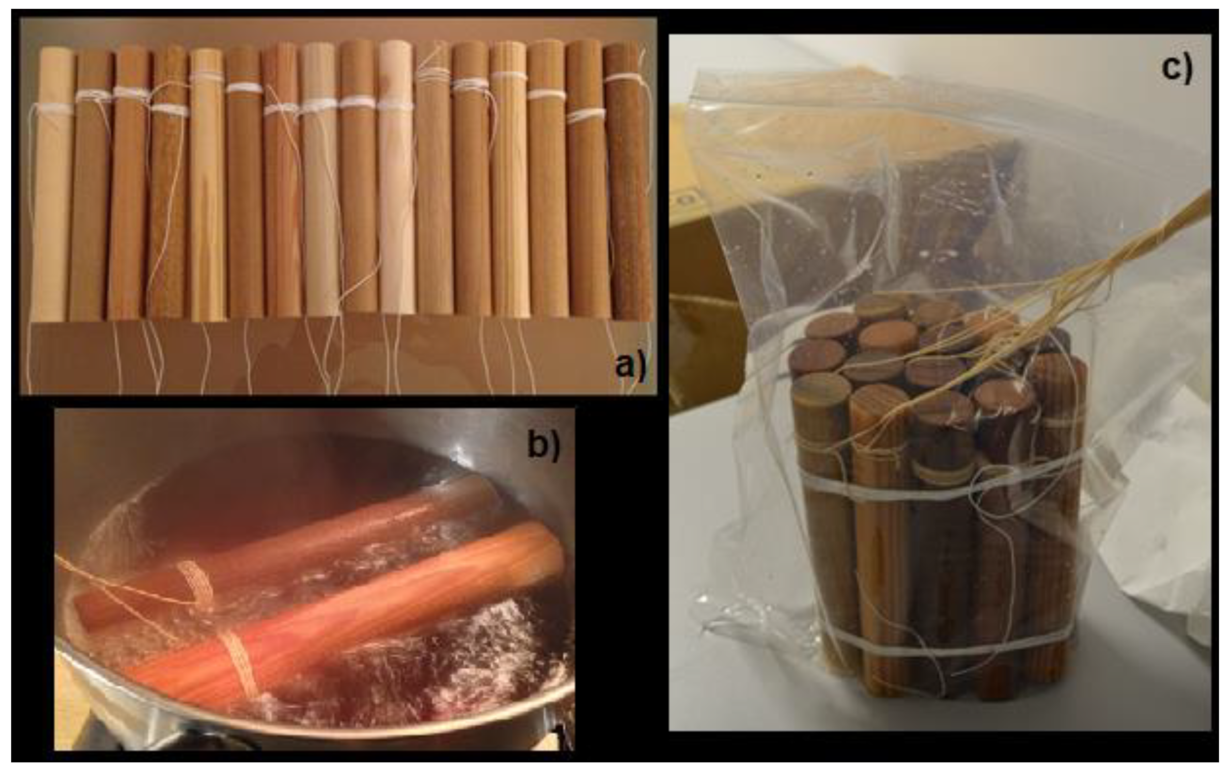
Thirty-two cylinders of wood with diameter d = (2.95 ± 0.05) cm and height h = (20.0 ± 0.1) cm were assembled to obtain two phantoms of sixteen cylinders, each with dimensions of about 15 cm × 12 cm × 20 cm (Figure 1 and

Table 1. Wood denominations of species analyzed in this work (right column) with the associated letter on the left to identify them.

Identification Letter	Wood Sample Species
A	Abura—Bahia (Mitragyna ciliata)
B	White Poplar (Populus alba)
C	Limba (Terminilia superba)
D	Red Spruce (Picea abies)
E	Silver Fir (Abies alba)
F	Anigrè (Aningeria altissima)
G	Silver Fir (Abies alba)
H	Sessile Oak (Quercus petraea)
I	English Walnut—Common Walnut (Juglans nigra)
L	Anigrè (Aningeria altissima)
M	Sapele (Entandrophragma cylindricum)
N	Australian Red Cedar—Toona (Toona ciliata)
O	Virginia Pine—Scrub Pine american (Pinus ponderosa)
P	African Walnut—Dibetou (Lovoa trichilioides)
Q	Red Spruce (Picea abies)
R	Virginia Pine—Scrub Pine american (Pinus ponderosa)

). Pieces of the aforementioned wood cylinders were cut to obtain little samples, 2.5 cm in height, for mass and density measurements. Moreover, a waterlogged archaeological wood sample from the Roman port of 5th century AC found in the Piazza Municipio of Naples (Italy) was investigated. It is characterized by a diameter of 8.7 cm.

To obtain a full water-imbibed sample, a phantom made of sixteen wood specimens was properly and completely immersed in 5 L of distilled water (Figure 1). The container was covered with plastic wrap so that water could not evaporate, and dust particles could not contaminate the solution. Four days later, the wood samples were boiled in distilled water for 30 min to let water penetrate the wood more easily [45]. This procedure was repeated four times to bring most of the wooden cylinders to water saturation. A wood sample is considered saturated when it sinks in water. After the first boiling procedure, the A, I, M, N, and O specimens (Table 1) sank; the H specimen sank after two days from the first boiling procedure; the F, L, and P specimens sank after the fourth day. Differently, the B, C, D, E, G, and Q specimens never sank.

Another phantom of sixteen wood specimens was exposed for two weeks to a temperature of 24 °C and relative humidity (RH) of about 30%. These temperature and RH values were chosen to be equal to those of the room where the 3 T NMR scanner, used to investigate the wood samples, was installed.

Finally, the archaeological wood from the Roman port of 5th century AC found in the Piazza Municipio of Naples (Italy) was soaked in water at the time of its discovery and was immediately stored in a tub of water at the Central Institute of Restoration in Rome (ICR, Italy). The archaeological wood sample belonged to a mooring pole for boats in the ancient port of Naples. Therefore, it is made up of wood of a very abundant species in the surroundings of Naples of 5th century AC with very poor value. It has been identified as Ashwood [2,46] by optical microscopy investigation of its fragment.

2.2. Wood Density Measurement

The wood density, d, was obtained from the relation:

$$d=M/V,$$

(1)

where $M$ is the mass and $V$ is the volume.

The following procedure was used to obtain masses and volumes of all the investigated woods. Initially, the mass of empty weighing bottles was measured with an analytical balance BP211D Sartorius. Subsequently, the masses of the samples inserted in the weighing bottles were measured. The samples, in the appropriate open containers, were positioned inside the Universal Memmert Oven stove at a temperature of T = (103.5 ± 0.5) °C for 24 h. Then, the container was closed before extraction from the stove to prevent the wood from instantly absorbing the humidity present in the laboratory. Once the masses were measured, this procedure was repeated for a second time, to achieve 48 h of drying time. It is believed that by using the above procedure, the samples were released from most of the moisture present [45].

The obtained data were processed to calculate the mean mass value and the standard deviation (SD) before and after drying for 24 and 48 h. A t-test was then carried out to assess whether the differences in the masses before and after the drying cycles were significant. Once all the values of the masses were collected, the density of each species of the samples was calculated. The $M$ net mass of the samples was calculated as follows:

$$M=Mcp-Mps,$$

(2)

where $Mcp$ is the mass of the weighing bottles with the inserted samples, measured after the drying procedure, and $Mps$ is the mass only of the weighing bottles. The error on the mass was obtained by summing the absolute errors of the two subtracted quantities. Then, the volume of samples was evaluated according to the relation:

$$V=A · h,$$

(3)

where A is the base area and h is the height.

The mean volume of each sample was equal to $V=\left(17.1 \pm 1.3\right)$ cm³.

2.3. MRI Acquisition

A Philips Achieva 3.0 T X-series (Philips Healthcare, Amsterdam, the Netherlands) clinical scanner, equipped with a 3T static magnetic field, high-performing imaging gradients (800 mT/m maximum gradient strength with 200 mT/m sloping ramp), and a FreeWave 32 SENSE-HEAD canals coil was used.

For the 16 modern water-soaked samples, the T₂-weighted (T₂-w), T₂*-weighted (T₂*-w), and T₁-weighted (T₁-w) images were performed using, respectively, a turbo spin echo (TSE) sequence, a gradient echo (fast field echo, FFE) sequence, and an inversion recovery turbo spin echo (IRTSE) sequence. All the parameters used, such as echo time (TE), repetition time (TR), inversion recovery time (IR), in-plane resolution (R), number of slices (N° slices), slice thickness (STK), number of scans (NS), matrix size (MTX) and field of view (FOV) are reported in

Table 2. Acquisition protocols used for the 16 modern water-soaked samples.

Purpose	High-Resolution Images			T2, T2* and T1 Measurement
Sequence	T2-TSE	T2*-FFE	T1-IRTSE	T2-TSE	T1-IRTSE	T2*-FFE
TE or TEs (ms)	16	4	30	10, 21, 32, 42, 52, 63, 74, 84, 94, 105	20	3, 9, 15, 21, 27, 33, 39, 45, 51, 57
IR or IRs (ms)	-	-	1800	-	100, 200, 400, 800, 1200, 1600, 1800	-
TR (ms)	1500	1000	2000	1500	2000	2000
STK (mm)	5	5	3	5	5	5
N° slices	20	20	20	20	20	20
NS	1	2	1	1	1	4
MTX (mm2)	880 × 880	1024 × 1024	1024 × 1024	640 × 640	672 × 672	288 × 288
FOV (mm2)	260 × 260	260 × 260	260 × 260	260 × 260	260 × 260	260 × 260
In-plane resolution, R (mm2)	0.29 × 0.29	0.25 × 0.25	0.25 × 0.25	0.41 × 0.41	0.39 × 0.39	0.90 × 0.90

. All images were acquired in axial view, i.e., along the transversal plane, which is perpendicular to vessels and tracheids [17]. Moreover, on the same 16 wood samples, the T₂, T_1, and T₂* values were measured by using, respectively, an axial-view TSE sequence, an axial-view IRTSE sequence, and an axial-view FFE sequence, and all the parameters are reported in Table 2. T₂* measurement was performed on both the water-soaked and 30% RH samples, whereas T₁ and T₂ measurements were performed only on water-soaked woods. T₂-w images were also used to obtain a 3D reconstruction of the 16 modern water-soaked samples.

To carry out MRI on the archaeological wood sample and to obtain its T₂*-w and T₂-w images, respectively, a gradient echo (FFE) sequence and a TSE sequence were used, and their acquisition parameters are reported in

Table 3. Acquisition protocols used for the archaeological waterlogged wood sample.

Purpose	High-Resolution Images and T2, T2* Measure		3D Reconstruction
Sequence	T2-TSE	T2*-FFE	T1-FFE
TE or TEs (ms)	20, 40, 60, 80, 100	8, 16, 23	6
TR (ms)	500	112	25
STK (mm)	1.5	1.5	1.5
Slice Gap (mm)	1.5	1.5	0
N° slices	5	3	60
NS	2	2	2
MTX (mm2)	1024 × 1024	1024 × 1024	512 × 512
FOV (mm2)	240 × 240	240 × 240	240 × 240
R (mm2)	0.23 × 0.23	0.23 × 0.23	0.47 × 0.47

. Finally, a 3D T₁-FFE sequence by selecting the parameters reported in Table 3 was applied to obtain T₁-w images in all sample volumes to perform the 3D reconstruction.

2.4. CT Acquisition

A Somatom Sensation 16 (Siemens Healthcare, Erlangen, Germany) with a gantry opening of 70 cm was used to obtain X-ray computed tomography (CT) images from the archeological waterlogged wood sample and a sample comprised of sixteen wood species. The spiral acquisition was performed using the following parameters: 180 mAs, 120 kV, slice thickness of 0.6 mm, FOV = 216 × 216 mm², matrix 512 × 512, pitch 0.70 mm B60s smooth Kernels.

2.5. MRI Data Processing

The Philips DICOM Viewer version R3.0 SP15 (Philips Healthcare, Amsterdam, the Netherlands) software was used to analyze Digital Imaging and Communications in Medicine (DICOM) images and to obtain regions of interest (ROI) in each wood cylinder of soaked and dry samples.

For each of the sixteen-soaked cylinders, some slices with homogeneous areas in signal intensity were chosen. For each slice, an ROI was selected manually to obtain the signal intensity, taking care that within that slice, each sample maintained a region of interest of similar extension.

To obtain proton density S(0), T_2, and T₂* maps, a homemade script of Matlab (MATLAB 9.0 R2016a (MathWorks Inc.) © 2023–2023 The MathWorks, Inc., Natick, MA, USA was used. In each image voxel, the following functions [21] were used to fit the S(TE) data from T₂ and T₂* acquisitions performed at different TEs:

S(TE) = S(0) exp(−TE/T₂) + c,

(4)

where c is a constant that considers the noise level. Moreover, by using Equation (4), we quantified T₂ and T₂* in each selected ROI while using the following relation:

S(IR) = S(0) [1 − 2exp(−IR/T₁)],

(5)

where S(IR) is the signal intensity, and at time IR we obtained the T₁ value.

To obtain the 3D reconstruction from 2D MRI of 16 cylinders-soaked phantoms we using the software generally employed in neuroimaging research: MRIcro, dcm2nii, mricron, and mricron32.

dcm2nii was used to convert the DICOM image to Neuroimaging Informatics Technology Initiative (NIfTI). In addition, to obtain 3D reconstruction from 2D T₁-w MRI of the archaeological sample, the Horos 2.4.1 software (iCat Solutions Ltd., Horos^™, Markham, ON, USA) a free, open-source medical image viewer, was used.

2.6. Statistical Analysis

The average values of the T₁, T₂, and T₂* parameters extracted from each slice were obtained with their standard deviations (SDs). Pearson’s correlation (R) was used to study linear correlations between variables. A p-value (p) less than 0.05 was considered for statistical significance.

2.7. 3D Rendering

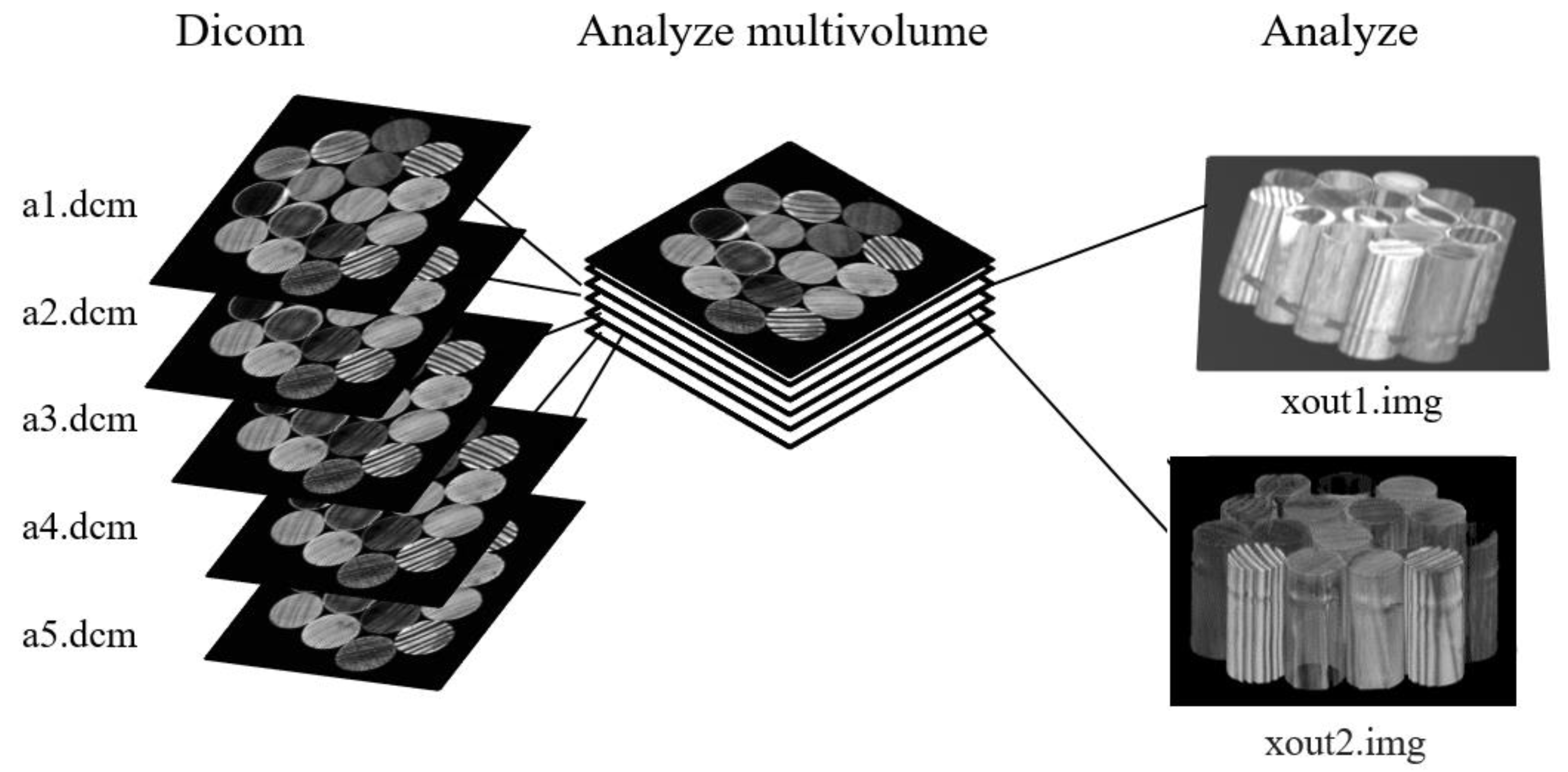
For the wood cylinders, 3D reconstruction from 2D MRI was obtained using the software generally employed in neuroimaging research: MRIcro, dcm2nii, mricron, and mricron32.

To use the MRIcro software that allows you to obtain 3D rendering from a series of 2D images, the 2D images in DICOM format must be converted to the SPM2 (3D Analyze hdr/img) format using the dcm2ii software. Then, it is necessary to convert the images from SPM2 format into SPM5 format (3D NlfTI1 Analyze hdr/img), as displayed in Figure 1.

Statistical Parametric Mapping (SPM) uses the NlfTI (Neuroimaging Informatics Technology Initiative) image format. The NlfTI format was created with the aim of accelerating the development and improving the usefulness of IT tools related to neuroimaging. This format includes information on image orientation. Figure 2 shows a schematic representation of DICOM files conversion in SPM format (Analyze hdr/img) to be used with MRIcro software. Using MRIcro, it is possible to visualize all 3 different orientations of the sample. The volume rendering is a technique for visualizing a 2D projection of a 3D sample. Using the Render option of MRIcro, we had access to the 3D image of wood samples. It was possible to choose the area/surface ratio to select the minimum voxel intensity that would be counted as part of the volume. It was possible to select the value of the surface depth that indicated how many voxels below the surface were averaged to determine the intensity of the surface. Moreover, roto-translation parameters: azimuth angle (Azimuth) and elevation (Elevation), are parameters that change the position of the observed sample by rotating it on the horizontal and vertical planes, respectively. The sample display option allowed us to choose whether to display one of the three image orientations or all three at the same time.

In addition, to obtain 3D reconstruction from 2D T₁-w MRI of the archaeological sample, the Horos software, a free, open-source medical image viewer, was used.

3. Results and Discussions

In this study, multiparametric high-resolution NMR images of different wood species were acquired using a clinical scanner operating at 3 T. In the first step, 16 different species of soaked wood were used (Figure 1 and Table 1) to test the potential of 2D and 3D MRI for the diagnosis of wood species and to distinguish hardwood and softwood. Then, the relaxation times of soaked and environmental humidity wood samples were quantified. Finally, an archeological wood sample was investigated.

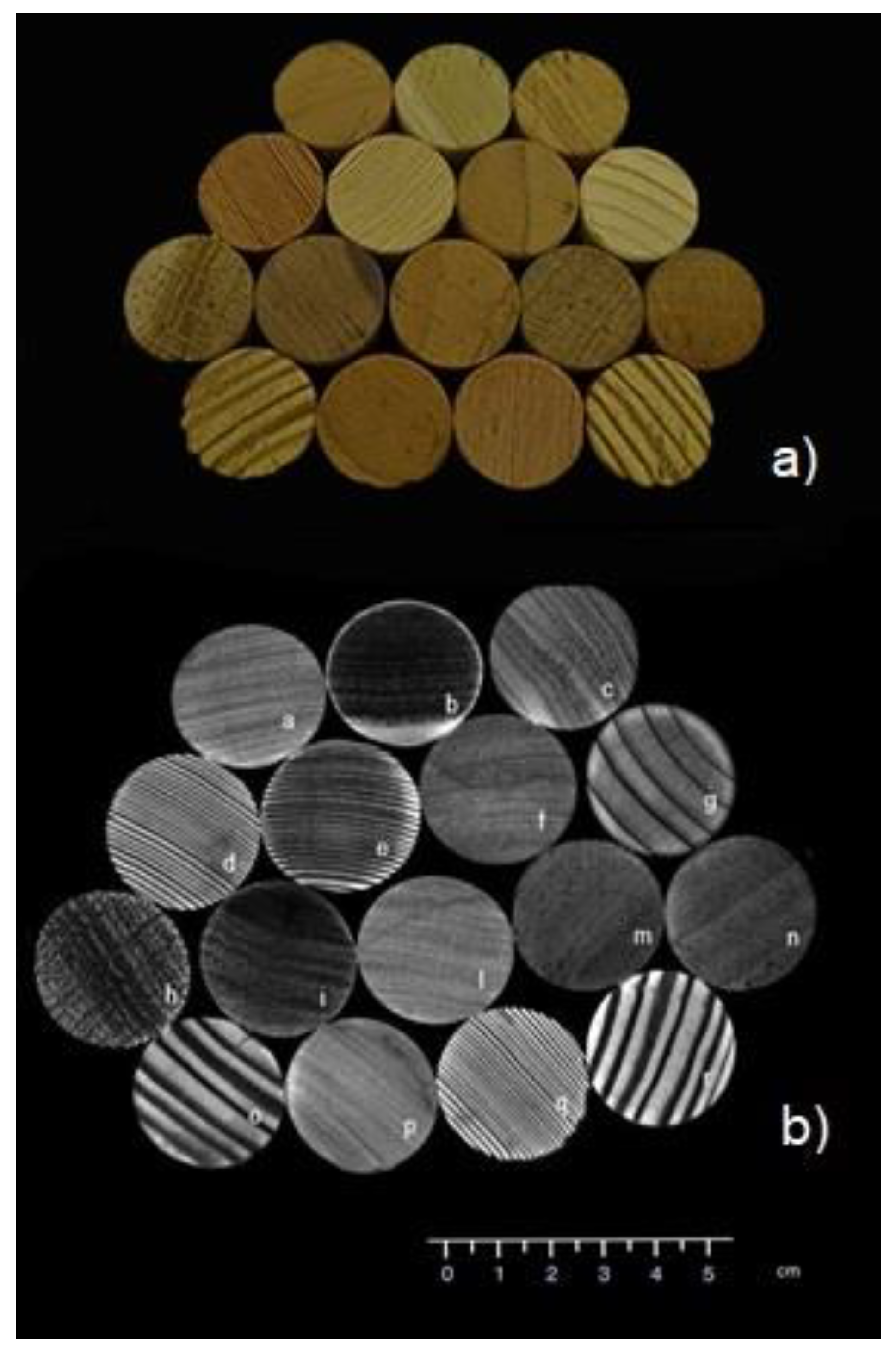
By comparing macroscopic wood characteristics observed with MRI to the standard macroscopic wood identification keys [2,46] usually utilized by wood experts, it was possible to perform an NMR survey with images and measurements of the relaxation times of 16 different wood species characterized by different microstructures. Figure 3 shows, at the top a photo, one of the 16 wooden cylinders sample used in this work and, at the bottom, its T₂-weighted NMR image (T₂-w image), obtained with an in-plane resolution of 250 × 250 μm². 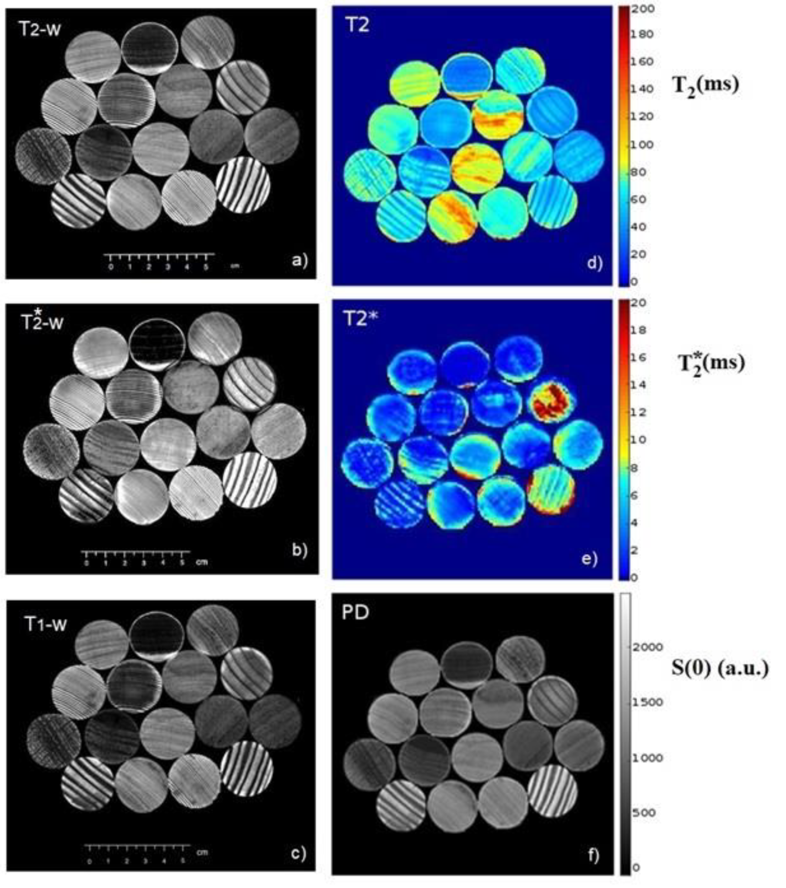Moreover, Figure 4 shows a multiparametric MRI of the same sample, where T₂-w, T₂*-w, and T₁-w images are displayed in Figure 4a–c, respectively. On the right side of Figure 4, T₂, T₂*, and proton density (PD) maps are reported in Figure 4d–f, respectively.

The timbers investigated in this work belong mainly to two categories: those of the Gymnosperms (known as softwoods [47]) and those of the Angiosperms (known as hardwoods [48]). These two groups present important structural differences. The softwoods, because of the presence of the same elements that perform more functions (tracheids), are called “homoxils” [47]. Differently, the hardwoods are called “eteroxils” [48] because they consist mainly of two different types of cells, one with mechanical function (fibers), and the other with conduction function (vessels). Regarding the wooden cylinders investigated in this work, the cross-section was mainly analyzed the because there are distinguishable growth rings, knots, regions of deterioration, and other structural characteristics of the wood [49].

To the best of our knowledge, the images in Figure 3b and Figure 4 are the first images of wood samples acquired with an in-plane resolution of 250 × 250 μm², using an NMR clinical scanner. Images are of good quality due to the high NMR signal intensity and the specific multiparametric contrast provided by the different NMR acquisition sequences. Moreover, the possibility of manipulating the images by medical software without loss of quality allows for enhancing image contrast differences that highlight anatomical characteristics which are peculiar to the two main groups, hardwood and softwood. To obtain such high-quality images, the bulk water in vessels and tracheids was exploited due to its longer T₂ relaxation as compared with that of bound water in wood parenchyma, which is about 1 ms or less (see

Table 4. T₁ and T₂ of 100% soaked wood specimens.

Wood Specimen 1	T1 (ms)		T2 (ms)
	Value	SD	Value	SD
A	265	±5	87.3	±0.1
B	570	±15	20.4	±0.6
C	287	±6	62.8	±1.1
D	338	±20	71.5	±1.9
E	85	±2	46.8	±1.0
F	324	±5	117.5	±0.3
G	82.5	±0.5	38.0	±0.6
H	519	±3	55.9	±1.3
I	466	±4	35.6	±0.1
L	313	±5	125.6	±0.2
M	577	±4	64.8	±0.2
N	446	±4	34.4	±0.2
O	82	±1	46.0	±1.2

¹ The correspondence between letter and wood essence is shown in Table 1.

and

Table 5. T₂* of 100% soaked and RH = 30% wood specimens.

T2* (ms)
Wood Specimen 1	Waterlogged		Environmental Humidity (RH = 30%)
	Value	SD	Value	SD
A	11.9	±0.3
B	2.08	±0.05
C	5.5	±0.2	0.34	±0.06
D	10.3	±1.0	0.42	±0.07
E	4.9	±0.1
F	6.5	±0.1
G	15.82	±0.05	0.40	±0.02
H	5.95	±0.04	0.58	±0.01
I	9.0	±0.1
L	10.8	±0.3
M	12.8	±0.5	0.742	±0.004
N	11.4	±0.4	0.475	±0.004
O	12.0	±0.2

¹ The correspondence between letter and wood essence is shown in Table 1.

and Figure 4d,e). This allowed the evaluation with high-definition images of the internal sections of the material and, in particular, the differentiation between hardwood and softwood groups was reached without taking or cutting out the samples. This characteristic of non-invasiveness is fundamental for cultural heritage investigations. Therefore, thanks to the inhomogeneous distribution of water [50], for each species of wood, it is easy to distinguish macroscopic anatomical characteristics such as growth rings, veins, parenchyma rays, texture, the difference between sapwood and heartwood, possible knots, and plant defects, without having to dissect the samples. In particular, some darker areas and black spots appearing in the T₂*-w image of some species (Mitragyna ciliata, Aningeria altissima, Entandrophragma cylindricum, Toona ciliata, Pinus ponderosa) may be due to magnetic field inhomogeneities generated by air pockets confined in the pores, or by paramagnetic substances present in the wood [13,35,43].

The T₂ map (Figure 4d) allows us to immediately identify areas where the water is more mobile (longer T₂), and therefore, where wood is less dense and more homogeneous in structure. The T₂* map allows us to identify areas characterized by a higher inhomogeneity of magnetic field (lower T₂* values) due to the magnetic susceptibility difference between adjacent wood tissue [51] (such as water in vessels and vessels cell membrane). These are highly heterogeneous areas and/or areas with the presence of paramagnetic agents or heavy metals that contribute to decreasing the value of the T₂* parameter [43]. The proton density (PD) map shows the spatial distribution of the S(0) parameter which is related to the NMR signal intensity without the relaxation effects (see Equation (4)). Therefore, the PD map highlights the amount of water in the wood.

We report the results and discussions for the different investigated wood species in the following.

3.1. Softwoods

In the images obtained in this work (Figure 3b and Figure 4a–c), the annual rings are well marked in softwood (D, E, G, O, Q, and R). In the growth rings, the light gray tones of the image voxels are ascribed to the beginning of the vegetative growth (earlywood), characterized by cellular elements with a broad lumen and thin cell walls to allow better management of nutrients from the roots to the foliage [47]. From the images, it appears that these areas have been mainly filled with free water. A very strong signal, recognizable in NMR images with whiter voxels, identifies porous areas in which there is a greater penetration of bulk water in large pores. Instead, the darker voxels areas, represent the latewood, characterized by cells with small diameters and thick cell walls, which therefore have a lower water content that is more closely bound to cell walls [13,47,52,53].

Considering the pines (Pinus ponderosa), samples O and R in Table 1 are characterized by well distinguishable annual rings, with a quite abrupt transition between earlywood and latewood [46,47]. It can be noted that latewood occupies from one-third to one-half of the annual ring. By zooming the image, resin canals are visible in the latewood portions or around them. From the high-resolution images, it is possible to notice a medium texture typical of all the species of pines, found especially in the T₂*-weighed image.

In the spruces (Picea abies), samples D and Q, it is possible to notice that the growth rings are well evident even if thinner than those of the pines. Furthermore, there is a gradual passage between the early and late zone. By enlarging the image, the rings in some parts are slightly wavy. All these features are perfectly in agreement with the known structure of spruce reported in the IAWA list [47] and with the high-field and high-resolution images reported in the Capuani et al. [17] paper.

In the silver firs (Abies alba), samples E and G, the annual rings are distinct, and the two samples have a variable amplitude, probably due to different growth conditions. This causes a different absorption of water, well observable in the T₂* map displayed in Figure 4e. Here, the map of sample G is characterized by T₂* values greater than the average values of the other samples (see also Table 5). This suggests a more homogeneous and less compact structure of the silver firs as compared with the other wood samples. The typical silver firs texture [47] that goes gradually from medium to fine is also observable [52].

3.2. Hardwoods

One of the main characteristics to identify hardwood is the arrangement of the pores (i.e., the transversal/cross-section of the vessels) [48,52]. There are three main groups based on the size and arrangement of the vessels in the annual ring. Ring-porous wood, semi-ring porous wood, and diffuse-porous wood [46,54]. The first one presents vessels in earlywood, cells with conduction functions, larger than those in latewood. This consists of a well defined zone in which there is an abrupt transition between earlywood and latewood which is visible. Semi-ring porous wood could present vessels in earlywood larger than the one in latewood or it could not. It presents a gradual transition between earlywood and latewood. The last type presents vessels with the same diameter. This characteristic is typical of tropical and temperate species [55].

In the sessile oak (Quercus petraea), sample H, by zooming the image, the presence of multiseriate parenchymal rays and the ring-porous, typical of deciduous oaks, can be distinguished. The texture is coarse and, thanks to the possibility of medical software to measure dimensions, a diameter of the vessels in the earlywood is estimated to be about 300 μm.

In the English walnut (Juglans nigra), which corresponds to sample I, it is possible to recognize a semi-ring porous, with identifiable growth rings in the image weighed in T₂*. This species presents a medium texture.

Some samples, such as Sapele (Entandrophragma cylindricum) and Australian red cedar (Toona ciliata), respectively, M and N, observed with a greater magnification, present a diffuse-porous ring and an indistinct growth ring boundary, especially in the T₂*-w images. There is a medium texture with vessels visible to the naked eye and a diameter of about 200–300 μm.

In white poplar (Populus alba, sample B), the different water absorption in the wood structure causes darker and lighter voxel-area stripes (Figure 3 and Figure 4a–c), as already highlighted for silver fir. There are annual rings that can be identified in the T₂*-w, T₂-w, and T₁-w images, their trend is quite regular, and the amplitude is about 2 mm. However, in general, all the image voxels of sample B are darker as compared with the voxels associated with all the other wood samples. Indeed, white poplar is characterized by denser parenchyma and a larger parenchyma area as compared with the vessels area [17,46,52]. White poplar is composed of a smaller number of pores and voids than silver fir and a greater number of walls and barriers which contain more trapped water [52]. All these characteristics indicate that water penetrates with extreme difficulty in poplar and the water inside the parenchyma is characterized by much shorter T₂ and T₂* relaxation times than the average relaxation times measured in other wood species. All these characteristics reduce the MRI signal intensity of water in poplar as compared with the signal intensity observed in other wood species.

On the market, there are species of different origins, which, although not part of the auglandaceae family, are usually improperly referred to in the common language as “walnut” [56]. Examples are the abura (Mitragyna ciliata, A), the aniegrè (Aningeria altissima, F-L), the limba (Terminilia superba, C), and the dibetou (Lovoa trichilioides, P). The textures of these species, belonging to different families, range from coarse (C) to medium (F-L and P) or fine (A). The border of the growth rings can be more or less distinct from the images. This type of hardwood could be referred to as diffuse-porous wood species.

3.3. Relaxation Times and Wood Density

T₁ and T₂ mean values obtained from each homogeneous ROI selected in each slice of the 16 soaked wood species sample are reported in Table 4, whereas in Table 5, T₂* mean values of 16 soaked wood species sample and 16 wood species sample at RH = 30% are listed. Finally, the wood density (in kg/m³) for all sixteen wood species is reported in

Table 6. Wood density obtained for each wood species.

Sample 1	Density (kg/m3)
A	530 ± 40
B	480 ± 40
C	480 ± 40
D	540 ± 40
E	350 ± 40
F	560 ± 40
G	350 ± 30
H	630 ± 50
I	680 ± 50
L	520 ± 40
M	550 ± 40
N	520 ± 40
O	510 ± 40
P	550 ± 40
Q	520 ± 40
R	530 ± 40

¹ The correspondence between the letter and wood species is shown in Table 1.

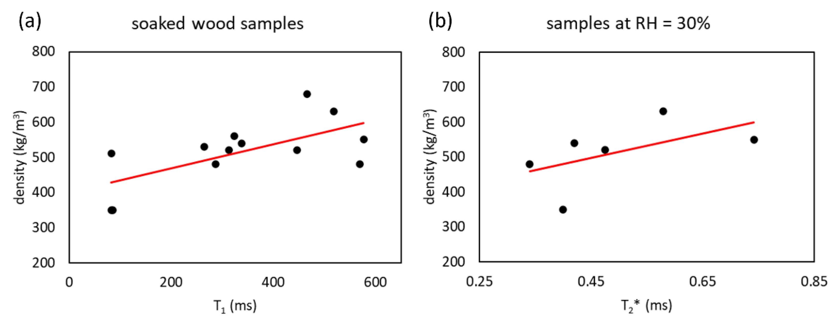
. The density values in Table 6 are in agreement with those reported in the literature [56]. On the one hand, no significant correlation was found between T₂ and T₂* and wood density in the water-soaked wood sample. On the other hand, a significant correlation was found between T₁ and wood density (Pearson’s correlation (R) = 0.60, p-value (p) = 0.025) in the water-soaked wood samples (in agreement with references [52,57]), and between T₂* and wood density (R = 0.38, p = 0.045) in the wood samples at RH = 30%, as shown in Figure 5.

Some relaxation times of wood samples at RH = 30% could not be quantified due to poor NMR signal or high SD. When RH = 30%, there is poor water that wets the walls of vessels [58,59]. This water is strongly interacting with cell walls and membranes [42,57,58,60]. For this reason, the T₂* relaxation times are much shorter than those of the free water in the vessels [39,52]. Indeed, T₂* measured in wood at RH = 30% belongs to water molecules bound to the wood polymers present in the cell wall, and therefore, it can be used to extract information on the wood density since it depends on the overall lumen volume and cell wall volume fractions [52,61].

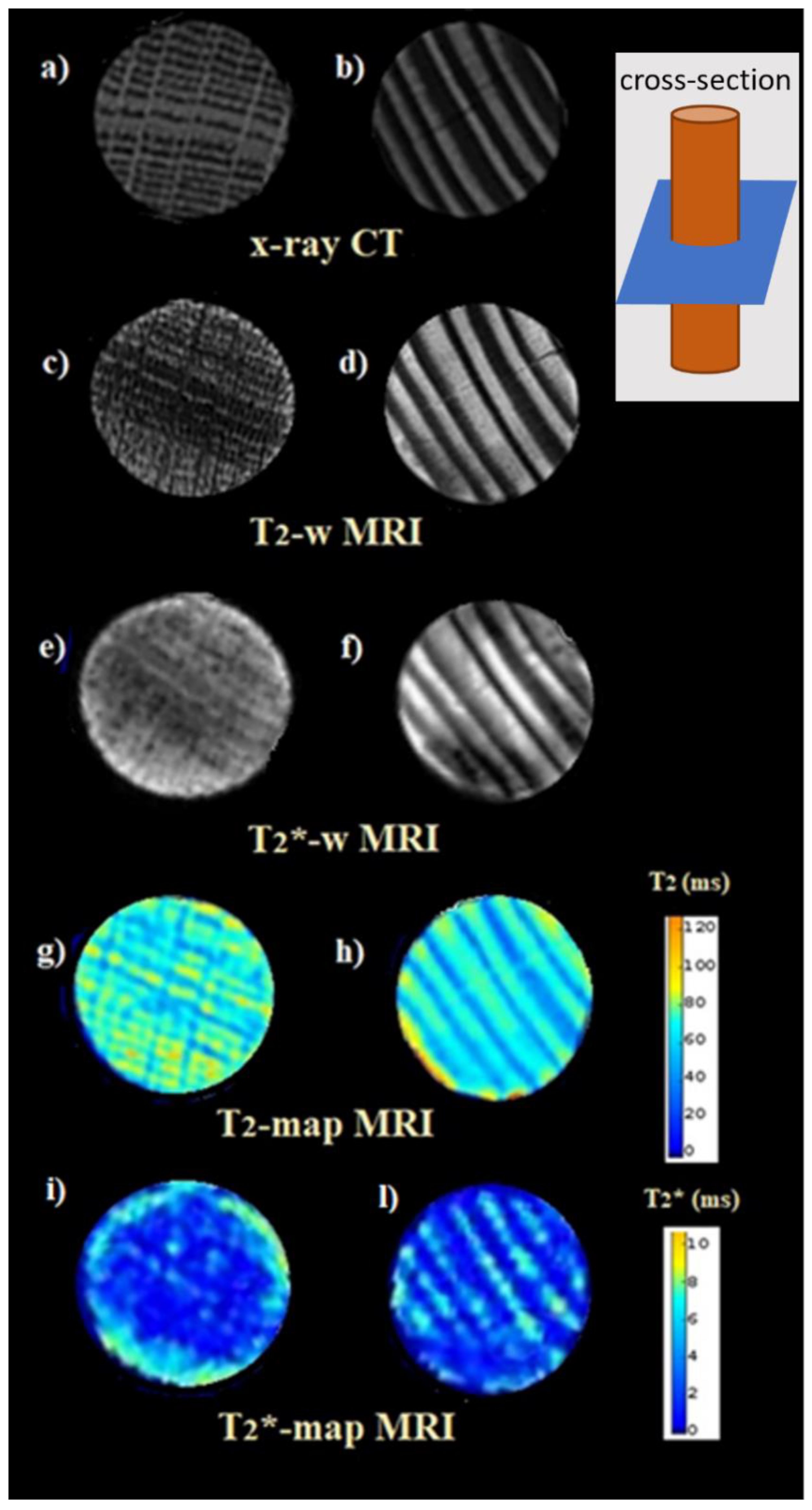
3.4. CT and Multiparametric MRI Comparison

Images comparison are displayed between one hardwood (Figure 6a,c,e,g,i), the Sessile Oak, and one softwood (Figure 6b,d,f,h,l), the Virginia Pine sample, obtained by CT scan (Figure 6a,b), T₂-w (Figure 6c,d), T₂*-w (Figure 6e,f), T₂-map (Figure 6g,h) and T₂-map (Figure 6i,l) MRI.

Apparently, the contrast of the X-ray CT images (Figure 6a,b) appears opposite as compared with that of the T₂-w images and T₂ maps (Figure 6c,d,g,h). The wood denser rings, which appear characterized by pixels lighter in the X-ray images, appear characterized by pixels darker in the NMR images. However, observing the T₂*-w (Figure 6e,f) and the T₂*-maps (Figure 6i,l), we realize that the contrast between X-ray and NMR images does not only follow the aforementioned simple rule. The T₂*-maps enhance the magnetic field inhomogeneities [17,51,62] generated by the magnetic susceptibility difference at the interface between different wooden tissues, wood and water, and wood and air, showing a decidedly different contrast as compared with what we observe in the X-ray images. In addition to this complementary information, as compared with that provided by X-rays, T₂*-w images are also sensitive to magnetic field inhomogeneities generated by paramagnetic substances and/or deposits of heavy metals [13,17,43]. This information is particularly useful in analyzing submerged archaeological wood, as we show later.

3.5. 3D Visualization from 2D MRI

Using MRIcro, it is possible to visualize all three different orientations (longitudinal, transversal, and sagittal) of the sample. In Figure 7, the screen capture image of the MRI obtained along the three different image views of a wood sample partially imbibed with water is displayed. As suggested by the example reported in Figure 7, using this MRIcro modality it is possible to monitor the water transport into vessels or other wood structures and evaluate their volume.

The 3D MRI surface rendering of the sample composed of sixteen different water-imbibed wood species (see Table 1 and Figure 2) is displayed in Figure 8. Using the view projection of the Render option of MRIcro software the sample at different orientations in space is observable. Brighter zones represent high-water content wood structures. The render option allows a change of the air/surface threshold and the surface depth to visualize 3D images at different image contrasts. An image with minimum surface/depth values and an image with high air/surface values are reported in Figure 8a,b, respectively; different values of the sharpness filter allow us, by zooming the image, to observe macroscopic differences among softwood and hardwood samples (Figure 8c,d).

3.6. 2D and 3D MRI of a Waterlogged Archeological Wood

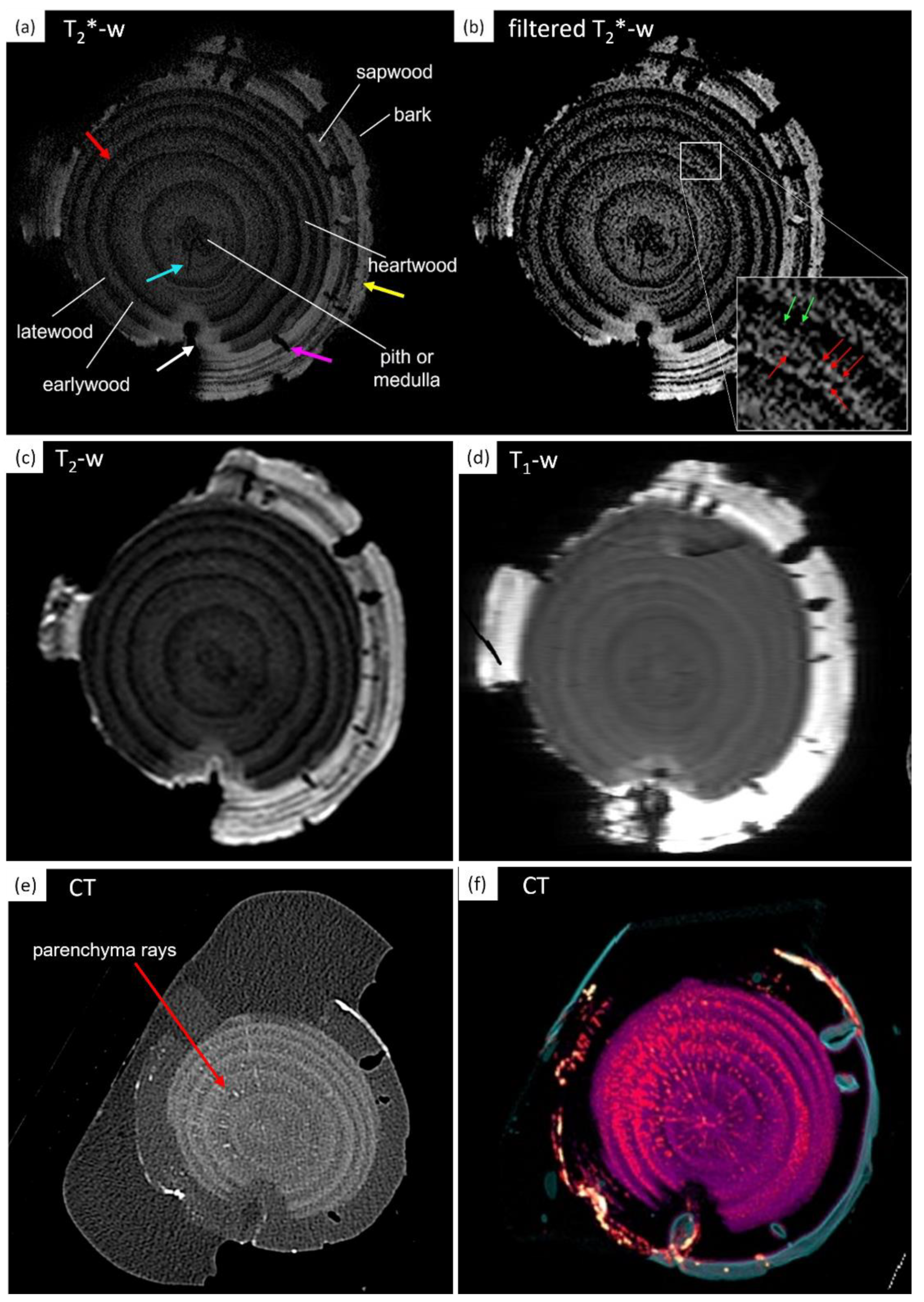
In Figure 9a–d, the T₂*-weighted, T₂-weighted, and T₁-weighted MR images together with CT images (Figure 9e,f) obtained by virtual sectioning the archeological wood sample along the transversal direction (i.e., perpendicular to the wood vessels and tracheids) are shown.

Earlywood and latewood are well visible in both the MR and the CT images, showing opposite image contrast differences. Heartwood and sapwood could be distinguished in MR images (Figure 9a–d) but not well in CT images (Figure 9e,f). However, parenchyma rays are only visible in CT and CT color-coded images whereas, in general, the CT multiplanar reconstruction image (MPR) shows less tissue contrast than MRI, but it confirms MRI water absorption differences in sapwood and heartwood. Considering the inverse relation between wood density and wood porosity and the linear relation between HU and wood density, HU values measurements confirm that sapwood (characterized by 33 HU) adsorbs more water as compared with heartwood (characterized by 150 HU), as reported in the literature [63].

The MRI contrast differences, which depend on T₂, T₁, and magnetic field inhomogeneities [28] at the interface between different wood elements, allowed us to recognize wood macroscopic components, such as sapwood with lighter voxels and heartwood characterized by darker image voxels. This result indicates that the average water content of sapwood is greater than that of heartwood (i.e., the mean porosity and the mean size of pores in sapwood are larger than in heartwood). In Figure 9a,b, at the center of the wood cylinder, it is possible to see the pith or medulla characterized by quite dark voxels as compared with the surrounding image voxels, highlighting a weak NMR signal due to low water content and/or high paramagnetic substances that generate high field inhomogeneity (i.e., low T₂* values). However, by comparing MR and CT images, as the medulla is not well visible in the CT image, we can advance the hypothesis that the medulla is better highlighted in MR images (where it is characterized by darker voxels) due to field inhomogeneities caused by salts or heavy metals trapped in the wood structure [13,20,31,35,43]. Overall, the wood sample appears well preserved with some major fractures (pink arrow) and perforations (yellow arrow) visible in Figure 9a. Moreover, the pith shape and cracks (light-blue arrow) as well as the decayed zone in heartwood (white arrow) can be seen in Figure 9a. These features indicate that the wood sample suffered mechanical stress and microbial degradation.

All the aforementioned image contrast differences are enhanced by the filter applied to the MR image in Figure 9b. Considering that the T₂*-weighted MR image of Figure 9a,b was acquired at echo time (TE) = 1 ms, the structural components of wood that provide a dark contrast are characterized by water with a transversal relaxation time (T₂*) close to or shorter than 1 ms. Since a fast relaxation time T₂* indicates that water is confined inside small structures, we can infer the pores size of the above-mentioned components. At the microscopic level, this wood is characterized by porous rings with distinct boundaries (red arrow, Figure 9a). Each annual ring seems to have an abrupt transition from latewood to earlywood. Latewood exhibits darker voxels that can be ascribed to the smaller lumen size of its vessels, whereas earlywood has brighter voxels due to the greater vessel sizes. This is well shown in the filtered image of Figure 9b, wherein in the zoomed square it is possible to notice smaller vessels in latewood (green arrows) and larger vessels in earlywood (red arrows). The MR image of Figure 9a has a linear resolution of 250 µm, and therefore, the anatomical elements with sizes smaller than 250 µm are not well resolved. In any case, the image of the wood sample shows many white pixels indicating the presence of vessels with a cross-section not much less than 250 µm (see the insert in Figure 9b). In the literature [64,65] the cross-section of Ash’s vessels is about 150–250 microns. Moreover, it must be considered that often in archaeological wood the pores are larger due to decay.

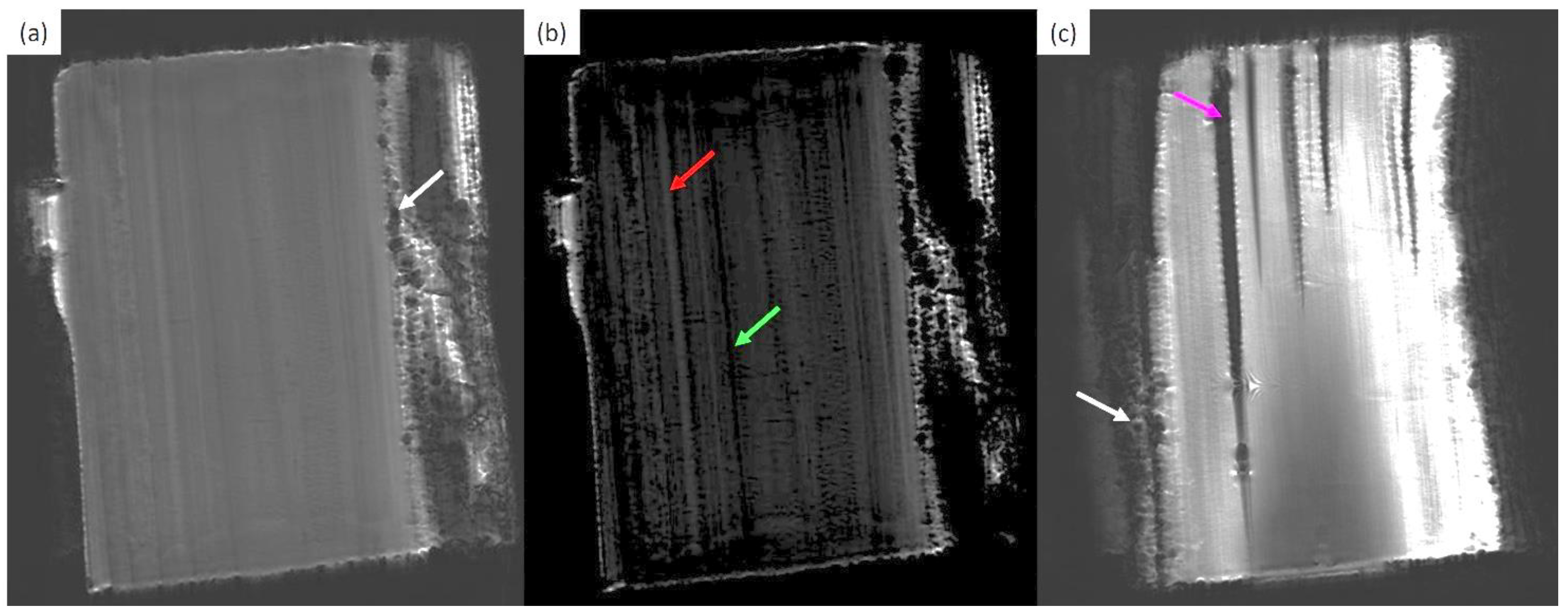
In Figure 10a, the T₂*-weighted MR image obtained by the longitudinal sectioning (i.e., parallel to the wood vessels) of the heartwood part of the archeological wood is shown. This image presents a strong degraded area on the right side with black spots (white arrow) that can be attributed to the degradation activity operated by microorganisms (fungi and bacteria) [38]. The degraded area exhibits a lighter contrast and is well separated from the rest of the sample, characterized by a more homogeneous grey color. We can identify the narrowest degraded area characterized by brighter white voxels in MR images as sapwood (Figure 9 and Figure 10c) and the largest homogenous area characterized by gray voxels as heartwood (Figure 9 and Figure 10a,b).

The filtered image in Figure 10b helps us to discriminate between structures with contrast differences: vessels (red arrow) and the annual ring limit (green arrow). Moreover, the same T₂*-weighted longitudinal MR image was obtained from the outer zone of the wood (Figure 10c). Its average lighter contrast suggests that this section was cut from sapwood as also confirmed by the large fractures (pink arrow), which are in the outermost area of the sample corresponding to the sapwood (see Figure 9a). The sapwood section is also characterized by black spots due to biological decay (white arrow). The three MR images in Figure 10 suggest that the ancient wood is a hardwood composed of well-preserved heartwood and strongly degraded sapwood.

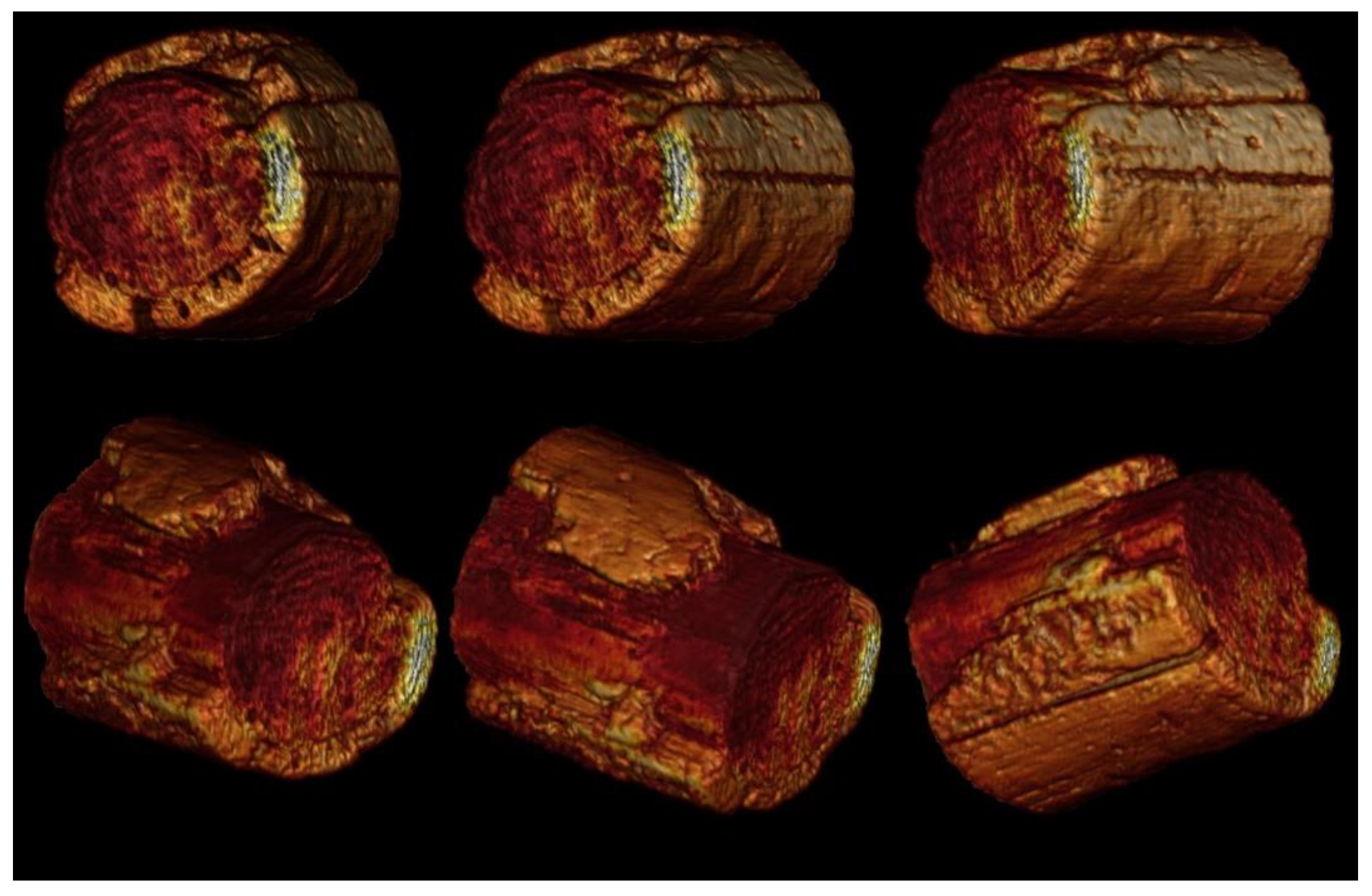
Figure 11 shows the 3D reconstruction of the archeological waterlogged wood obtained from all 2D image volumes. Figure 11 is composed of 3D images obtained using Horos, a free open-source medical image viewer. The 3D images come from a video showing the sample rotating around an axis, or another, which can be made using the 3D Viewer, the 3D Volume Rendering, and the movie option of the software. Just like in medical diagnostics, 3D imaging can help diagnose a wooden object. It is possible to evaluate the volumetric structure of the find to study its state of conservation or the technique used to make it. In Figure 11, it is possible to evaluate the state of conservation of the entire find. The lighter colors correspond to very porous, and therefore, not very dense wood with spaces filled with water. Darker colors indicate denser wood, with smaller pores and less water quantity. With the 3D visualization, it is possible to better evaluate, as compared with the observation of single 2D images, the erosion of the outer sapwood, which in some zones is completely missing.

4. Conclusions

This work highlights the possibility of carrying out diagnostics of wooden samples and archaeological wooden finds using MRI instrumentation and software for data processing employed in medical diagnostics. Several modern reference samples were analyzed and discussed to find a suitable methodology for archaeological waterlogged wood remains. Furthermore, for the first time, in this work NMR and CT images have been compared. The similar, different, and complementary information obtainable from both techniques was shown, suggesting the great potential of 2D and 3D MRI for the study and diagnosis of waterlogged wood. As reported and discussed in this paper, the MRI exam is particularly sensitive in discriminating “soft”, i.e., highly hydrated, woody tissues or wood structures filled with water (vessels, tracheids, hemicellulose). On the contrary, the image contrast provided by the CT allows the investigation of “hard” woody tissues, such as lignin and crystalline cellulose. On the one hand, the presence of water confuses the contrast differences provided by the X-rays in waterlogged wood images. On the other hand, MRI can highlight structures and features not visible by CT.

The combination of MRI and CT analyses allows to distinguish between hardwood and softwood directly on images and, at the same time, collect information about microstructure and preservation status through relaxometry measurements. Useful information about the dynamics of water or other substances inside samples, such as archaeological waterlogged woods, can be obtained. Moreover, in the case of conservation treatments, it could be a useful tool to choose the most suitable consolidant product or to evaluate its penetration.

In perspective, the images obtained with the combined CT-MRI approach could allow the creation of a type of “clinical file” of the wooden object with a detailed 3D reconstruction that could be an innovative tool for the digitalization of marine and waterlogged archaeological collections by using instrumentation widespread along the territory. These instruments are non-destructive, which is the most important requirement of diagnostic techniques for cultural heritage.