Abstract
Previous research on the effects of neighborhood crowding and soil moisture on tree height growth have been limited by time-consuming and sometimes inaccurate ground-based measurements of tree height. Recent developments in unmanned aerial vehicles (UAVs) allow detailed 3D point clouds of the canopy surface to be generated at relatively low cost. Using UAV-derived point clouds, we obtained height measurements of 4386 trees for the years 2019 and 2021. We also calculated four neighborhood crowding indices and a topography-based moisture index (depth-to-water) for these trees. Using initial tree height, neighborhood crowding indices and the depth-to-water index, we developed Bayesian hierarchical models to predict height growth for three tree species (Picea glauca (white spruce), Populus tremoluides (trembling aspen) and Pinus contorta (lodgepole pine)) across different stands. Bayes-R values of the final models were highest for white spruce (35%) followed by trembling aspen (28%) and lodgepole pine (25%). Model outputs showed that the effect of crowding and depth-to-water on height growth are limited and species-dependent, adding a maximum of 7% to the Bayes-R metric. Comparing different neighborhood crowding indices revealed that no index is clearly superior to others across all three species, as different neighborhood crowding indices resulted in only minor differences in model performance. While height growth can be partially explained by aerially derived neighborhood crowding indices and the depth-to-water index, future studies should focus on identifying relevant site characteristics to predict tree growth with greater accuracy.
1. Introduction
Predicting tree height growth is important to accurately modelling forest dynamics and its relationship to ecosystem services such as timber yield or carbon sequestration [1,2]. Tree height growth is a complex process, as it is influenced by a variety of factors related to physical (aspect, slope), chemical (nutrients) and biological (competition, symbiosis) conditions. Previous efforts to model height growth have aimed to capture those factors using predictors such as initial tree size and indices that describe site factors and local competition [3,4,5,6]. One way to measure local competition is through the assessment of neighborhood crowding, which mainly captures competition for light but can also reflect depletion of soil nutrients or water [7]. The effects of neighborhood crowding on tree growth vary considerably across species, environmental conditions, and regions. For example, in tropical rainforests [7] found different effects of neighborhood crowding in South America than in Africa, while [8] found that effects can depend on the species of mycorrhiza that are associated with root systems.
Neighborhood crowding in forest stands can have various effects on the height growth of individual trees. Increased neighborhood crowding could cause trees to prioritize height growth as a strategy for reducing their level of shading. Such effects are well known for other plants and have been reported in previous literature [9]. However, increased neighborhood crowding can also lead to decreased height growth rates because of strong competition between trees, which results in a few trees acquiring most of the available resources at their neighbors’ expense [8]. Whether neighborhood crowding has net positive or negative effect on a subject tree’s height growth depends on multiple factors that make clear predictions difficult. Furthermore, height growth is strongly related to life history traits such as longevity, regeneration patterns, or shade tolerance, resulting in varying responses when trees experience crowding [10].
Studies measuring neighborhood crowding with aerial canopy height data have used crowding indices based on ones calculated from ground-based data [11,12,13]. Ma et al. [11] estimated crowding by quantifying the percentage of competitive crown area in a subject tree’s neighborhood. Pedersen et al. and Lo et al [12,13] used sized-based, distance-dependent indices based on the angle formed between a point at a specified height of the subject tree and each neighboring tree’s crown surface. Vanderwel et al. [14] adopted the indices of the above-mentioned studies and compared their ability to explain variation in radial tree growth to traditional ground-based indices. Results indicated that aerial competition indices can be at least as effective as traditional ground-based metrics for measuring the effects of local crowding on radial growth.
Another important variable for estimating growth rates of trees is soil moisture [15,16]. Depending on species and the amount of soil water, changes in soil moisture can have either positive or negative effects on growth rates. Several proxy indices for soil moisture have been developed based on remotely sensed topographic information, including depth-to-water. The depth-to-water index [17] is defined as the cumulative slope along the least-cost pathway from a cell in the landscape to the nearest flow channel. It can can be represented by a map indicating potential wet areas, which are closely correlated with soil moisture regimes [18,19,20]. Although not yet widely used, the depth-to-water index is regarded as a promising metric for modelling the effects of soil moisture on tree growth [21].
Height growth responses of trees can vary considerably between species and stands. Species differ in their maximum annual height increments, which can be seen when comparing previous studies on a variety of species [22,23,24]. Moreover, depending on genetics and their associated life history traits, species will react differently to shortages in available resources [10]. Furthermore, stand conditions can be defined by an infinite number of variables that may influence a tree’s height growth. Such variables include neighborhood crowding and soil moisture, but also for example, species composition, nutrient levels, slope, or aspect. Interactions between different variables can influence the shape of relationship they have on growth rates. For instance, lodgepole pine (Pinus contorta) is less shade intolerant when located in dry locations [25,26], and growth rates of white spruce (Picea glauca) depend on a stand’s species composition [27].
Previous studies have compared UAV-based height measurements to traditional ground-based methods and found a low and acceptable range of error [28,29,30,31,32]. Although many studies have successfully measured tree height and inter-annual height growth using UAV-derived point clouds [32,33,34,35,36,37,38], we are not aware of any that have measured tree height growth over more than one year or evaluated effects of neighborhood crowding to date. Here, we use a set of neighborhood crowding indices derived from aerial canopy data to measure the effect of crowding on the height growth of three tree species. We also evaluate whether tree height growth is related to water availability within individual stands. Specifically, we sought to determine how tree height growth is influenced by (1) neighbourhood crowding and (2) depth-to-water, and how these relationships vary among species and stands within a given landscape.
2. Materials and Methods
2.1. Study Area
Field data were collected in Cypress Hills Interprovincial Park, a 35,000 ha protected area located on the southern Alberta-Saskatchewan border in western Canada (49°40 N, 110°15 W). Elevations range from 1000–1463 m. The climatic zone of the park is characterized as sub-humid with a mean annual temperature of approximately 2 °C and a mean annual precipitation of 550 mm. Vegetation in the park is a mosaic of fescue prairie and forests, with forests covering approximately 54% of the park’s landscape [39]. Forests in Cypress Hills are outliers of the aspen parkland and coniferous forest zones that border the Northern Great Plains of Canada [40], and are dominated by white spruce, trembling aspen (Populus tremoluides) and lodgepole pine. The majority of stands originated between 1880 and 1890 following large fires [41]. White spruce is a shade and drought tolerant species that can retain water within its tissues by reducing physiological activity during dry conditions [42]. In the study region it can be found mostly at lower slopes and valleys near creeks or wet areas. Lodgepole pine is shade intolerant but drought tolerant. It requires fire to open its serotinous cones and create suitable conditions for seed germination and growth [43]. Throughout the park it is mostly found on drier sites at higher elevations. Trembling aspen is a clonal, light demanding broadleaf tree species that can exchange resources through root connections [44]. It occupies mostly mid-slope positions on sites with intermediate soil moisture [45,46].
2.2. Canopy Height Models
We obtained aerial data for twenty forest stands across the park, of which eight stands were dominated by trembling aspen, six were dominated by white spruce, and six were dominated by lodgepole pine (Figure 1). In the summers of 2019 and 2021 a DJI Matrice 200 v2 (Beijing, China) equipped with a Sentera AGX-710 multispectral sensor was flown to obtain aerial imagery of these stands (Figure 1). Those surveys were used to derive detailed canopy height models for each forest stand and its surroundings. Image acquisition flights were carried out according to recommendations of [47]. The UAV flew to a predetermined altitude 60 m above the canopy. The UAV repeatedly traversed a 150 m by 200 m rectangular area in a series of parallel flight lines that maintained >90% side and forward overlap between adjacent images. As it flew over the site, the UAV captured downward-facing photos approximately every 2 s with a single flight lasting 24 min on average. Each photo was georeferenced using the UAV’s GPS and GLONASS receivers. Photogrammetric software (Agisoft Metashape (v. 1.6.4, St. Petersburg, Russia)) was used to generate a high resolution orthophoto (5.1 ± 0.9 cm per pixel), digital elevation model (DEM), and digital surface model (DSM) for each stand. Canopy height models (CHM) were produced from the differences in elevation between each stand’s DEM and DSM.
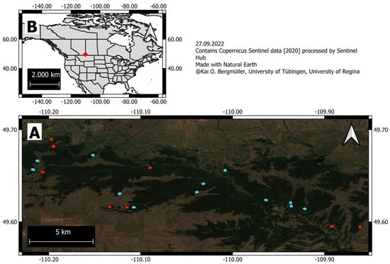
Figure 1.
(A) Location of 20 forest stands within Cypress Hill Interprovincial Park, coloured based on whether they were sampled for soil moisture (blue) or not (red). (B) Study area location within North America.
We used the orthophotos and CHMs to manually identify individual treetops within these stands, and to delineate the portion of each tree’s crown that contained its tallest point (Figure 2). Because single trees in the georeferenced data sets were not perfectly aligned between study years, the crown delineation process was done separately for 2019 and 2021 to avoid inaccurate tree height measurements. Due to the nature of UAV imagery understory trees could not be included. Orthophotos were used to identify tree species, resulting in 1695 white spruce, 1516 trembling aspen, and 1175 lodgepole pine.
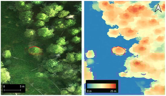
Figure 2.
Details from an orthophoto (left) and canopy height model (right). The red polygon shows the outline of the crown of a lodgepole pine that was manually delineated for height extraction.
Trees were chosen to have good visibility in the orthophotos and CHMs, so as to avoid mistakes in height extraction. Using the manually segmented tree crowns and the corresponding CHMs, we extracted the maximum height of each tree segment for the years 2019 and 2021. We calculated height growth rates for the two year period from the difference between these values.
2.3. Neighborhood Crowding Indices
Based on previous literature on remotely sensed neighborhood crowding indices, we derived four different indices that could be calculated from our CHM data. We first drew an annulus around each subject tree with a 15 m outer radius and 2 m inner radius. The 2 m inner radius was chosen to exclude the subject tree’s own crown, based on typical crown widths for the study area [14]. We then extracted the 2019 CHM values within the annulus for each subject tree and used these to calculate different indices. First, we calculated simply the mean canopy height in each area surrounding a specific tree (“mean canopy height”). Second, we calculated the canopy cover as the proportion of the CHM area which was above two meters in height (“canopy cover”). Third, we calculated the fraction of the canopy that was greater than 75% of the subject tree’s height in 2019 (“canopy above”). All of these indices were easy to calculate, but they did not account for the distance between each CHM pixel and the subject tree. Therefore, a fourth index was added to better account for the canopy’s spatial structure. We calculated the angle formed between a point at 75% of a subject tree’s height, and each pixel of the CHM in the previously defined surrounding area. We then calculated the mean sine function of these angles (“canopy angle”) (Table 1, Figure 3).

Table 1.
Summary of the chosen neighborhood crowding indices, showing equations, distance and size dependence as well as references.
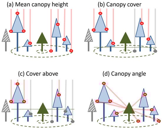
Figure 3.
Schematic illustrations for the four neighborhood crowding indices used in this study adapted from [14]. In each panel, a focal tree (solid green) is subject to competition from neighbours (blue outlined trees) present in a given area (green dashed circles). Neighbours that are outside of this area or do not meet particular criteria (grey hashed trees) are not included in calculations. Indices are derived from the height above ground of cells outside of the subject tree’s crown that meet particular criteria (pink vs. grey circles and lines).
2.4. Depth-to-Water Maps
DSMs were used to create topography-based depth-to-water maps (Figure 4). Calculations of depth-to-water maps for each forest stand followed the procedures described in [48] using the rgrass7 package in the R programming language, as well as Grass GIS [49,50]. The depth-to-water calculations depend on the value specified for the flow initiation area (FIA), and so we calculated depth-to-water maps corresponding to FIAs of 1.25 ha, 0.75 ha and 0.25 ha (Figure 5), which represent moisture conditions ranging from dry (1.25 ha) to wet (0.25 ha) soil. To determine an appropriate FIA value and validate the relationship between soil moisture and depth-to-water index, we measured soil moisture gravimetrically within twelve different forest stands in July 2022 (Figure 1). Four stands were chosen for each tree species to span the range of the calculated depth-to-water values. Each stand was divided into a four by three grid, and we collected soil samples at a depth of 20 cm at the centre of each grid cell. We then examined the relationship between soil moisture and depth-to-water using linear mixed effect models for different FIA values. Depth-to-water maps calculated with a FIA of 1.25 ha explained the most variation in soil moisture levels (Table 2). We therefore used these maps to extract the mean depth-to-water value within a 2 m radius of each individual tree.
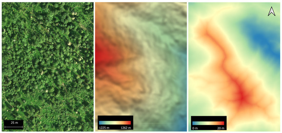
Figure 4.
Orthophoto (left), digital surface model (centre) and depth-to-water map (right) from an aspen-dominated forest stand.
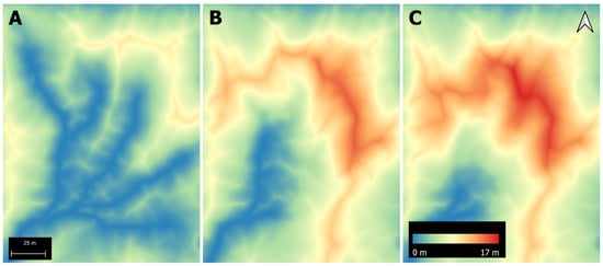
Figure 5.
Depth-to-water maps calculated with different flow initiation areas ((A) 0.25 ha, (B) 0.75 ha, (C) 1.25 ha) within an aspen-dominated forest stand.
Table 2.
Model fit summary for Bayesian linear mixed effect models (random slope and intercept across stands) that predicted soil moisture from depth-to-water maps with different flow initiation areas. 95% credible intervals for the effect of depth-to-water are shown, along with Bayes-R as a goodness-of-fit measure.
2.5. Growth Modelling
We developed a set of hierarchical Bayesian models to evaluate the influence of neighborhood crowding indices and the depth-to-water index on each species’ tree height growth. Separate models were created for each species with each model including stand-specific effects of neighbourhood crowding, tree height, and depth-to-water, as well as all two way interactions. Additionally, two base models were fitted to assess the influence of depth-to-water and neighborhood crowding: one including only the initial tree height as predictor, and the other adding the depth-to-water index but not neighborhood crowding. The growth models had the form:
where g is observed height growth, S is initial tree height, W and C are depth-to-water and neighbourhood crowding index values, respectively, i indexes the stand and j indexes the subject tree. The logarithmic transformation of initial tree height was chosen based on previous studies that have shown that size effects on growth become weaker as trees get larger [4,51]. All parameters were estimated as stand level random effects (i.e., random intercept and slope) that allowed for variation in their effects on height growth among stands. With these random effects at the stand level, we sought to account for possible differences in growth patterns between sites that may have been related to factors such as soil nutrient levels, exposure, or elevation. For the first base model (with initial tree height only), , , and were all set to zero. For the second base model (with initial tree height and depth-to-water), and were set to zero.
Each model was fit within a Bayesian framework using the package brms in the R programming language [49,52]. Distributional assumptions (normality, variance homogenity) and predictor independence were confirmed by inspection of raw data and residual plots. We tested for collinearity among predictor variables using their pairwise Pearson correlation coefficients. Absence of influential outliers was assured using the estimates for the shape parameter k of the generalized Pareto distribution using the default threshold of k > 0.7. Improper uniform priors were assigned to all model parameters. Samples were obtained from the posterior distribution of each model’s parameters by running four Markov chain Monte Carlo chains, each of which had 2000 warmup iterations, which were discarded, and 4000 sampling iterations.
Six different models were fit per species to evaluate the influence of four different neighborhood crowding indices and the depth-to-water index on tree height growth. These 18 models were fit separately to the available growth data for white spruce, trembling aspen and lodgepole pine. After model fitting we calculated the leave-one-out cross-validation information criterion (LOO) using Pareto smoothed importance sampling to estimate the out-of-sample predictive accuracy of each model [53].
We report estimated effect size ± SE as well as 95% credible intervals. If 95% credible intervals do not overlap zero then the corresponding predictors are reported as having a meaningful effect on height growth rates. Effects were also checked visually, as the presence of interactions makes it difficult to interpret main effects directly.
3. Results
3.1. Data Summary
Initial tree heights ranged from approximately 3–31 m (Figure 6). White spruce heights had the largest range. Trembling aspen, the smallest tree in the study, had generally lower heights than white spruce and lodgepole pine. Unlike the other two species, very few small (<10 m) lodgepole pine trees were present in the data set. Growth rates in the two-year study period were highest for white spruce, ranging from −0.9 m to 4.9 m. Pine growth rates ranged from −1.2 m to 4.4 m while trembling aspen growth ranged from −1.4 m to 4.6 m. Mean growth rates were highest for white spruce (approximately 1 m), while the average growth of aspen and pine were lower (approximately 0.4–0.5 m).
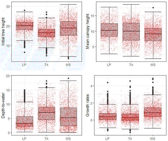
Figure 6.
Summary showing Box-Whisker plots for all predictor variables as well as tree height growth rates for each species (LP: lodgepole pine; TA: trembling aspen; WS: white spruce). Red dots represent individual data points.
3.2. Model Performance and Predictor Analysis
Base models using log transformed initial tree height as the only predictor variable were consistently ranked as the least informative across all species (Table 3). However, based on those models initial tree height had a consistent negative relationship with height growth. Effects were strongest for lodgepole pine (; 95% credible interval −1.38, −0.24), followed by white spruce (; −0.96, −0.54) and trembling aspen (; −1.10, −0.02). Base models that accounted for depth-to-water (but not neighbourhood crowding) performed much better than those with initial tree height only, but not as well as those that included neighbourhood crowding as a predictor (Table 3).
Table 3.
Summary of the differences in ELPD values for each species using different neighborhood crowding indices, based on the loo criterion. The model with highest ELPD-diff value is expected to have the best out-of-sample predictive performance.
No single neighborhood crowding index emerged as clearly superior to all others (Table 3). Mean canopy height performed well for white spruce, being ranked as the top model for that species. Canopy cover outperformed mean canopy height for lodgepole pine, and had similarly good performance to mean canopy height for white spruce. Canopy angle was ranked first for trembling aspen, but differences in ELPD values were <4 in comparison to mean canopy height, which is considered a small difference [53]. Canopy above never ranked as a top model for any species. Goodness-of-fit evaluation using Bayes-R showed that the largest share of variation in height growth (17%–27%) was explained by a subject tree’s initial height (Table 4). Adding depth-to-water as a predictor improved model performance by 2%–7%, with trembling aspen and white spruce showing the greatest improvements in fit. Neighborhood crowding produced little increase in Bayes-R for white spruce (0%–1%), but improved Bayes-R values somewhat more for lodgepole pine and trembling aspen (1%–4%). Variation in Bayes-R between neighborhood crowding indices within a species were small, ranging from only 1%–2%. The final height growth models performed best for white spruce (maximum 35% variation explained), followed by trembling aspen (28%) and lodgepole pine (25%) (Table 4).
Table 4.
Bayes-R values for the six height growth models for each species.
Based on ELPD and Bayes-R values, canopy cover was chosen as the final model for lodgepole pine and mean canopy height was chosen for white spruce and trembling aspen. Mean canopy height also showed a meaningful interaction with initial tree height (Table 5): smaller trees grow faster in less crowded neighborhoods, but slower as crowding increases, compared to tall trees (Figure 7). Consequently, height growth of small trembling aspen is affected negatively by increased crowding, whereas larger trees show a positive relationship between height growth and crowding. This relationship is unique for trembling aspen, as the other species showed no comparable interaction. Furthermore, an interaction between log transformed initial tree height and the depth-to-water index had a meaningful effect on trembling aspen’s height growth rates (Table 5). Small aspen trees grew faster in drier areas, reflecting a positive relationship between depth-to-water and height growth (Figure 7). Conversely, tall aspen trees grew faster in wetter areas than they did in drier areas. Again these effects are unique to trembling aspen, as the other species showed no comparable interaction. A third meaningful interaction was observed between the depth-to-water index and neighborhood crowding for lodgepole pine trees (Table 5): height growth of pine trees responded positively to crowding in drier areas, but not in wetter ones (Figure 7).
Table 5.
Parameter estimates of the final model for each species.
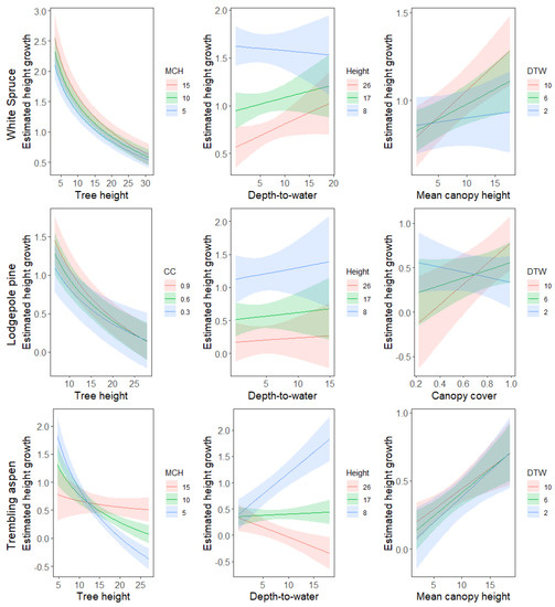
Figure 7.
Posterior mean predictions (±1 standard error) of height growth by species, tree height (height), depth-to-water (DTW), and neighbourhood crowding. Note that the axes have different scales across panels.
3.3. Stand Analysis
The random effects terms in the models allowed us to examine how the effects of tree size, neighborhood crowding and soil moisture varied among stands (Figure 8). The negative relationship between initial height and height growth was observed in all stands for white spruce and lodgepole pine. The effect of initial height was more variable among stands for trembling aspen, perhaps because it was influenced by interactions with neighborhood crowding and water availability (Figure 7). Extrapolating site-specific relationships between initial height and height growth it appears that white spruce trees do not reach their maximum height before 30 m, whereas the majority of lodgepole pine and trembling aspen stands reach a maximum height between 20 m and 30 m.
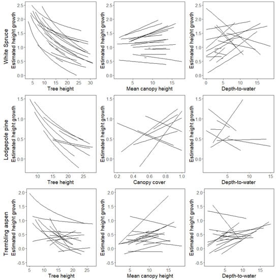
Figure 8.
Stand-specific relationships between predicted tree height growth and initial tree height (left), neighborhood crowding (centre), and depth-to-water (right) for each tree species. Note that the axes have different scales across panels.
Site-specific effects of neighborhood crowding and depth-to-water were not consistent, and included positive, negative, and neutral relationships for all three species (Figure 8). However, one notable pattern was that crowding had a positive effect in white spruce sites with faster height growth, but little effect in white spruce sites with slower height growth.
4. Discussion
To our knowledge, our study is the first to (1) estimate tree height growth rates over multiple years using UAV-derived CHMs; (2) evaluate the effect of neighborhood crowding on tree height growth based on aerial canopy data from UAVs; and (3) evaluate the usefulness of the depth-to-water index as a predictor variable for tree height growth rates. These advances have been made possible by recent developments in UAV technology that have opened new opportunities for modelling canopy structure from aerial imagery [14]. High-resolution CHMs can provide extensive data on tree heights more efficiently than ground-based measurements, and contribute detailed information on a subject tree’s neighborhood, which may serve as a proxy for the amount of competition that a tree experiences from its neighbors. Although the depth-to-water index has been applied successfully in different research areas, its value remains to be proven for predicting rates of tree growth.
Our comparison of different neighborhood crowding indices for predicting tree height growth revealed that there is no clearly superior index across the three species we studied. Canopy height has been previously used to predict stand attributes from airborne laser scanning data [54,55] and to predict radial tree growth rates [14]. For height growth we found that mean canopy height was most useful for trembling aspen, but that canopy cover was a better crowding metric for lodgepole pine (Table 3). White spruce did not show major improvements when including neighborhood crowding indices, which indicates that height growth rates for this species are relatively insensitive to competition.
4.1. Tree Size
Height growth rates across all species generally decreased with increasing tree size. The decrease in growth rates became weaker as trees approach their maximum height (Figure 7), as has been reported elsewhere [4,51]. However, the increase in growth rates from younger to medium-aged trees that has been found in other studies was not seen here, as very young trees are not often visible in UAV imagery and so were not well-represented in the dataset. By visually extrapolating site-specific relationships between initial height and height growth (Figure 8), we informally estimated maximum heights for each species. The estimated maximum heights of trembling aspen and lodgepole pine (20–30 m) were similar to previous reported values [23,56]. Maximum heights for white spruce were estimated to be much taller, perhaps exceeding 30 m [23].
4.2. Neighborhood Crowding Indices
Although the relationship between crowding and height growth varied somewhat across sites (Figure 8), increased neighborhood crowding generally seemed to stimulate height growth to avoid shading from surrounding trees. Such effects have been previously reported in studies of other plants [9]. Hara et al. [10] suggested that shade intolerant species located in crowded stands allocate resources to height rather than radial growth, in contrast to shade tolerant species. Furthermore, effects of crowding can depend on species and stand conditions.
We found that the effect of neighborhood crowding on height growth could depend on several factors. Lodgepole pine growth rates in wet sites (indicated by low depth-to-water values) were mostly unaffected by canopy cover, but in drier sites they showed faster growth rates under increased crowding (Figure 7). Newsome et al. [57] reported greater competitive effects of tall aspen on lodgepole pine in wetter, more productive sites, which is likely related to increased shade tolerance of lodgepole pine in dry sites [25,26]. Hence, competition associated with increased crowding negatively affects height growth in wet sites, whilst pines in dry sites are less prone to competition. Nevertheless, water seems to be a limiting factor for height growth rates at dry sites, as pines surrounded by few competitors still benefitted from increased water availability (Figure 7).
The height growth of short aspen trees decreased with increased crowding, but for taller trees the opposite effect was observed (Figure 7, Table 5). Small trees in locations with lower mean canopy height values are less prone to shading effects from neighboring trees [58]. Furthermore, competition for nutrients is likely less severe as there are fewer or smaller trees consuming resources. Large trees are less susceptible to shading by neighboring trees due to the size-asymmetric competition for light [58], and so competition should have a weaker effect on tall trees. At the same time, crowded locations may be associated with favorable stand conditions that enable trees to grow faster compared to locations with poorer conditions. For example, [46] reported increased survival of trembling aspen when it was surrounded by tall neighbours.
It is important to note that our dataset consisted only of overstory trees, as smaller understory trees cannot be seen from above. The height growth of smaller understory trees might be more sensitive to increased canopy height than that of canopy trees. Vanderwel et al. [14] reported that the effects of neighborhood crowding on radial growth rates were strongest for trees approximately 6 m high. Trees this size were very rare in the dataset (Figure 6), and so our results may underestimate effects of crowding for the whole population.
4.3. Depth-to-Water
Depth-to-water values had a meaningful influence on growth rates for lodgepole pine and trembling aspen. For both species, the direction of its effect depended on other variables. The effects of depth-to-water for lodgepole pine were linked to neighborhood crowding, as discussed above. Short aspen grew more slowly in wetter areas, but tall aspen grew faster in wetter areas (Figure 7). Reduced growth rates of short aspen in the Cypress Hills region could be related to a decreased competitive ability in relation to white spruce, which favours wet stands in the study area [46,59]. Decreased growth rates of large trees under drier conditions could be a sign of height limitation resulting from a lack of water.
Whether there is a positive or negative relationship between growth rates and depth-to-water was highly site dependent (Figure 8). Varying relationships between sites make it difficult to identify general patterns, which may be why our model did not report meaningful overall effects of depth-to-water for white spruce even though model performance improves when that variable is included. It is also possible that a larger FIA could produce depth-to-water maps that are more closely related to soil moisture levels, and that have stronger relationships with height growth. Readers should also keep in mind that the depth-to-water index is based on the topography omitting other relevant parameters such as forest density, litter depth, or mechanical composition. Owing to this simplification soil moisture may have stronger relationships with height growth than the depth-to-water index indicates.
4.4. Potential Sources of Error
Mean growth rates of trembling aspen and lodgepole pine were similar to previously reported averages [23,24], but the comparatively high growth rates for white spruce were not consistent with previous research [22]. Furthermore, while some negative values of growth rates can be explained by changing water pressures, defoliation, or fractures there is a degree of error associated with tree height measurements. Although we did not measure tree height estimation errors in our data, a number of other studies have investigated sources of error in aerial data [28,29,30,31]. Dempewolf et al. [32] reported increased error rates due to wind-induced movement of tree tops, as well as difficulties in developing accurate DSMs for dense forest stands. Low leaf cover and changing lighting conditions can also decrease measurement accuracy [47,60]. Such sources of errors are generally small when measuring individual tree heights, but can lead to a larger relative error when tree heights are compared at different times. To minimize errors, it can help to ensure similar flight conditions over multiple years. However, it can be difficult to carefully control for weather conditions especially when multiple sites are surveyed over a limited time period.
5. Conclusions
Our study showed that tree height growth decreased with initial height, and varied considerably between different sites. Neighborhood crowding and a depth-to-water index explained additional variation, but their effects were weaker, less consistent and species dependent. Competition related to crowding had little effect on height growth and could only be seen for some sites, in contrast to a previous study using the same crowding indices to predict radial growth [14]. This supports previous research, which has found height growth rates to be insensitive to competition compared to other tree parameters [61]. However, interactions between predictors determined whether they have a net positive or negative effect. Hence, generalizing statements about a single predictor are difficult to make, as complex models are needed to accurately model tree height growth. Further research should seek to identify other potential factors (such as soil or nutrients) that influence height growth and can account for the variability we found across different stands. Future studies should also seek to strengthen the correlation between a proxy index and soil moisture, either by testing a wider range of FIA’s regarding depth-to-water or using other indices. Aerial imaging offers a promising approach for modelling tree height growth, particularly if measurement errors across repeated surveys can be reduced through standardized flight conditions that minimize effects of lighting and wind.
Author Contributions
Conceptualization, M.C.V. and K.O.B.; Formal Analysis, K.O.B.; Data Curation, K.O.B. and M.C.V.; Writing—Original Draft Preparation, K.O.B.; Writing—Review & Editing, K.O.B. and M.C.V.; Visualization, K.O.B.; Supervision, M.C.V.; Project Administration, M.C.V.; Funding Acquisition, M.C.V. All authors have read and agreed to the published version of the manuscript.
Funding
This research was funded by the Natural Sciences and Engineering Research Council of Canada (funding number: RGPIN-2021-02521) and a PROMOS award from the German Academic Exchange Service to K.O.B.
Data Availability Statement
The data presented in this study are openly available on FigShare at https://doi.org/10.6084/m9.figshare.21774704 (accessed on 23 December 2022). The R code that was used for the set of models is openly available on GitHub at https://t.ly/Kb_l (accessed on 23 December 2022).
Acknowledgments
Many thanks to Christiane Zarfl for her valuable comments on the manuscript and her support during the creation of this work. Thank you to Imogen Mould for helping collecting soil samples and to Rebecca Dunkleberger, Kyle Cuthbert, Rebecca Bzdell and Dominick Smarda for the collection of drone data.
Conflicts of Interest
The authors declare no conflict of interest.
Abbreviations
The following abbreviations are used in this manuscript:
| CHM | Canopy height model |
| DEM | Digital elevation model |
| DSM | Digital surface model |
| ELPD | The theoretical expected log pointwise predictive density |
| FIA | Flow initiation area |
| LOO | Leave one out cross-validation information criterion |
| UAV | Unmanned aerial vehicle |
| MDPI | Multidisciplinary Digital Publishing Institute |
| DOAJ | Directory of open access journals |
References
- Jose, S.; Bardhan, S. Agroforestry for biomass production and carbon sequestration: An overview. Agrofor. Syst. 2012, 86, 105–111. [Google Scholar] [CrossRef]
- Hall, D.B.; Clutter, M. Multivariate multilevel nonlinear mixed effects models for timber yield predictions. Biometrics 2004, 60, 16–24. [Google Scholar] [CrossRef] [PubMed]
- Briseño-Reyes, J.; Corral-Rivas, J.J.; Solis-Moreno, R.; Padilla-Martínez, J.R.; Vega-Nieva, D.J.; López-Serrano, P.M.; Vargas-Larreta, B.; Diéguez-Aranda, U.; Quiñonez-Barraza, G.; López-Sánchez, C.A. Individual Tree Diameter and Height Growth Models for 30 Tree Species in Mixed-Species and Uneven-Aged Forests of Mexico. Forests 2020, 11, 429. [Google Scholar] [CrossRef]
- Nothdurft, A.; Kublin, E.; Lappi, J. A non-linear hierarchical mixed model to describe tree height growth. Eur. J. For. Res. 2006, 125, 281–289. [Google Scholar] [CrossRef]
- Jiang, L.; Li, Y. Application of Nonlinear Mixed-Effects Modeling Approach in Tree Height Prediction. J. Comput. 2010, 5, 1575–1581. [Google Scholar] [CrossRef]
- Ritchie, M.W.; Hann, D.W. Development of a tree height growth model for Douglas-fir. For. Ecol. Manag. 1986, 15, 135–145. [Google Scholar] [CrossRef]
- Rozendaal, D.M.A.; Phillips, O.L.; Lewis, S.L.; Affum-Baffoe, K.; Alvarez-Davila, E.; Andrade, A.; Aragão, L.E.O.C.; Araujo-Murakami, A.; Baker, T.R.; Bánki, O.; et al. Competition influences tree growth, but not mortality, across environmental gradients in Amazonia and tropical Africa. Ecology 2020, 101, e03052. [Google Scholar] [CrossRef]
- Ren, J.; Fang, S.; Lin, G.; Lin, F.; Yuan, Z.; Ye, J.; Wang, X.; Hao, Z.; Fortunel, C. Tree growth response to soil nutrients and neighborhood crowding varies between mycorrhizal types in an old-growth temperate forest. Oecologia 2021, 197, 523–535. [Google Scholar] [CrossRef]
- El-Gizawy, A.; Gomaa, H.; El-Habbasha, K.; Mohamed, S. Effect of different shading levels on tomato plants 1. Growth, flowering and chemical composition. Acta Horticult. 1993. [Google Scholar] [CrossRef]
- Hara, T.; Kimura, M.; Kikuzawa, K. Growth patterns of tree height and stem diameter in populations of Abies veitchii, A. mariesii and Betula ermanii. J. Ecol. 1991, 79, 1085–1098. [Google Scholar] [CrossRef]
- Ma, Q.; Su, Y.; Tao, S.; Guo, Q. Quantifying individual tree growth and tree competition using bi-temporal airborne laser scanning data: A case study in the Sierra Nevada Mountains, California. Int. J. Digit. Earth 2018, 11, 485–503. [Google Scholar] [CrossRef]
- Østergaard Pedersen, R.; Bollandsås, O.M.; Gobakken, T.; Næsset, E. Deriving individual tree competition indices from airborne laser scanning. For. Ecol. Manag. 2012, 280, 150–165. [Google Scholar] [CrossRef]
- Lo, C.S.; Lin, C. Growth-competition-based stem diameter and volume modeling for tree-level forest inventory using airborne LiDAR data. IEEE Trans. Geosci. Remote Sens. 2012, 51, 2216–2226. [Google Scholar] [CrossRef]
- Vanderwel, M.C.; Lopez, E.L.; Sprott, A.H.; Khayyatkhoshnevis, P.; Shovon, T.A. Using aerial canopy data from UAVs to measure the effects of neighbourhood competition on individual tree growth. For. Ecol. Manag. 2020, 461, 117949. [Google Scholar] [CrossRef]
- Bassett, J.R. Tree growth as affected by soil moisture availability. Soil Sci. Soc. Am. J. 1964, 28, 436–438. [Google Scholar] [CrossRef]
- Silberstein, R.; Vertessy, R.; Morris, J.; Feikema, P. Modelling the effects of soil moisture and solute conditions on long-term tree growth and water use: A case study from the Shepparton irrigation area, Australia. Agric. Water Manag. 1999, 39, 283–315. [Google Scholar] [CrossRef]
- Murphy, P.N.; Ogilvie, J.; Connor, K.; Arp, P.A. Mapping wetlands: A comparison of two different approaches for New Brunswick, Canada. Wetlands 2007, 27, 846–854. [Google Scholar] [CrossRef]
- Murphy, P.; Ogilvie, J.; Arp, P. Topographic modelling of soil moisture conditions: A comparison and verification of two models. Eur. J. Soil Sci. 2009, 60, 94–109. [Google Scholar] [CrossRef]
- Oltean, G.S.; Comeau, P.G.; White, B. Linking the depth-to-water topographic index to soil moisture on boreal forest sites in Alberta. For. Sci. 2016, 62, 154–165. [Google Scholar] [CrossRef]
- Schönauer, M.; Väätäinen, K.; Prinz, R.; Lindeman, H.; Pszenny, D.; Jansen, M.; Maack, J.; Talbot, B.; Astrup, R.; Jaeger, D. Spatio-temporal prediction of soil moisture and soil strength by depth-to-water maps. Int. J. Appl. Earth Obs. Geoinf. 2021, 105, 102614. [Google Scholar] [CrossRef]
- Bjelanovic, I.; Comeau, P.G.; White, B. High resolution site index prediction in boreal forests using topographic and wet areas mapping attributes. Forests 2018, 9, 113. [Google Scholar] [CrossRef]
- Wang, G.; Marshall, P.; Klinka, K. Height growth pattern of white spruce in relation to site quality. For. Ecol. Manag. 1994, 68, 137–147. [Google Scholar] [CrossRef]
- Peterson, E.; Peterson, N.M. Ecology, Management, and Use of Aspen and Balsam Poplar in the Prairie Provinces; Canadian Electronic Library: Edmonton, AB, Canada, 1992. [Google Scholar]
- Amman, G.D. The role of the mountain pine beetle in lodgepole pine ecosystems: Impact on succession. In The Role of Arthropods in Forest Ecosystems; Springer: Berlin/Heidelberg, Germany, 1977; pp. 3–18. [Google Scholar]
- Carter, R.; Klinka, K. Variation in shade tolerance of Douglas fir, western hemlock, and western red cedar in coastal British Columbia. For. Ecol. Manag. 1992, 55, 87–105. [Google Scholar] [CrossRef]
- Williams, H.; Messier, C.; Kneeshaw, D.D. Effects of light availability and sapling size on the growth and crown morphology of understory Douglas-fir and lodgepole pine. Can. J. For. Res. 1999, 29, 222–231. [Google Scholar] [CrossRef]
- Man, R.; Greenway, K.J. Effects of soil moisture and species composition on growth and productivity of trembling aspen and white spruce in planted mixtures: 5-year results. New For. 2013, 44, 23–38. [Google Scholar] [CrossRef]
- Torres-Sánchez, J.; López-Granados, F.; Serrano, N.; Arquero, O.; Peña, J.M. High-throughput 3-D monitoring of agricultural-tree plantations with unmanned aerial vehicle (UAV) technology. PLoS ONE 2015, 10, e0130479. [Google Scholar] [CrossRef]
- Díaz-Varela, R.A.; De la Rosa, R.; León, L.; Zarco-Tejada, P.J. High-resolution airborne UAV imagery to assess olive tree crown parameters using 3D photo reconstruction: Application in breeding trials. Remote Sens. 2015, 7, 4213–4232. [Google Scholar] [CrossRef]
- Lisein, J.; Pierrot-Deseilligny, M.; Bonnet, S.; Lejeune, P. A photogrammetric workflow for the creation of a forest canopy height model from small unmanned aerial system imagery. Forests 2013, 4, 922–944. [Google Scholar] [CrossRef]
- Karpina, M.; Jarząbek-Rychard, M.; Tymków, P.; Borkowski, A.; Tymków, P.; Borkowski, A. UAV-based automatic tree growth measurement for biomass estimation. Int. Arch. Photogramm. Remote Sens. Spat. Inf. Sci. 2016, 8, 685–688. [Google Scholar] [CrossRef]
- Dempewolf, J.; Nagol, J.; Hein, S.; Thiel, C.; Zimmermann, R. Measurement of within-season tree height growth in a mixed forest stand using UAV imagery. Forests 2017, 8, 231. [Google Scholar] [CrossRef]
- Krause, S.; Sanders, T.G.; Mund, J.P.; Greve, K. UAV-based photogrammetric tree height measurement for intensive forest monitoring. Remote Sens. 2019, 11, 758. [Google Scholar] [CrossRef]
- Panagiotidis, D.; Abdollahnejad, A.; Surovỳ, P.; Chiteculo, V. Determining tree height and crown diameter from high-resolution UAV imagery. Int. J. Remote Sens. 2017, 38, 2392–2410. [Google Scholar] [CrossRef]
- Zarco-Tejada, P.J.; Diaz-Varela, R.; Angileri, V.; Loudjani, P. Tree height quantification using very high resolution imagery acquired from an unmanned aerial vehicle (UAV) and automatic 3D photo-reconstruction methods. Eur. J. Agron. 2014, 55, 89–99. [Google Scholar] [CrossRef]
- Moe, K.T.; Owari, T.; Furuya, N.; Hiroshima, T. Comparing individual tree height information derived from field surveys, LiDAR and UAV-DAP for high-value timber species in Northern Japan. Forests 2020, 11, 223. [Google Scholar] [CrossRef]
- Peña, J.M.; de Castro, A.I.; Torres-Sánchez, J.; Andújar, D.; San Martín, C.; Dorado, J.; Fernández-Quintanilla, C.; López-Granados, F. Estimating tree height and biomass of a poplar plantation with image-based UAV technology. AIMS Agric. Food 2018, 3, 313–326. [Google Scholar] [CrossRef]
- Zainuddin, K.; Jaffri, M.; Zainal, M.; Ghazali, N.; Samad, A. Verification test on ability to use low-cost UAV for quantifying tree height. In Proceedings of the 2016 IEEE 12th International Colloquium on Signal Processing & Its Applications (CSPA), Melaka, Malaysia, 4–6 March 2016; pp. 317–321. [Google Scholar]
- Robinov, L.; Hopkinson, C.; Vanderwel, M.C. Topographic Variation in Forest Expansion Processes across a Mosaic Landscape in Western Canada. Land 2021, 10, 1355. [Google Scholar] [CrossRef]
- Newsome, R.D.; Dix, R.L. The Forests of the Cypress Hills, Alberta and Saskatchewan, Canada. Am. Midl. Nat. 1968, 80, 118–185. [Google Scholar] [CrossRef]
- Strauss, L.R. Fire Frequency of the Cypress Hills West Block Forest; Faculty of Graduate Studies and Research, University of Regina: Regina, SK, Canada, 2002. [Google Scholar]
- Grossnickle, S.C. Ecophysiology of Northern Spruce Species: The Performance of Planted Seedlings; NRC Research Press: Ottawa, ON, Canada, 2000. [Google Scholar]
- MacDonald, G.; Cwynar, L.C. Post-glacial population growth rates of Pinus contorta ssp. latifolia in western Canada. J. Ecol. 1991, 79, 417–429. [Google Scholar] [CrossRef]
- Peltzer, D.A. Does clonal integration improve competitive ability? A test using aspen (Populus tremuloides [Salicaceae]) invasion into prairie. Am. J. Bot. 2002, 89, 494–499. [Google Scholar] [CrossRef]
- Sauchyn, M.A.; Sauchyn, D.J. A continuous record of Holocene pollen from Harris Lake, southwestern Saskatchewan, Canada. Palaeogeogr. Palaeoclimatol. Palaeoecol. 1991, 88, 13–23. [Google Scholar] [CrossRef]
- Shovon, T.A.; Sprott, A.; Gagnon, D.; Vanderwel, M.C. Using imagery from unmanned aerial vehicles to investigate variation in snag frequency among forest stands. For. Ecol. Manag. 2022, 511, 120138. [Google Scholar] [CrossRef]
- Dandois, J.P.; Olano, M.; Ellis, E.C. Optimal Altitude, Overlap, and Weather Conditions for Computer Vision UAV Estimates of Forest Structure. Remote Sens. 2015, 7, 13895–13920. [Google Scholar] [CrossRef]
- Schönauer, M.; Maack, J. R-Code for Calculating Depth-to-Water (DTW) Maps Using GRASS GIS; Zenodo: Geneva, Switzerland, 2021. [Google Scholar] [CrossRef]
- R Core Team. R: A Language and Environment for Statistical Computing; R Foundation for Statistical Computing: Vienna, Austria, 2020. [Google Scholar]
- Awaida, A.; Westervelt, J. Geographic Resources Analysis Support System (GRASS GIS). USA: Geographic Resources Analysis Support System (GRASS GIS) Software. 2020. Available online: https://grass.osgeo.org/ (accessed on 30 December 2022).
- Bowman, D.M.J.S.; Brienen, R.J.W.; Gloor, E.; Phillips, O.L.; Prior, L.D. Detecting trends in tree growth: Not so simple. Trends Plant Sci. 2013, 18, 11–17. [Google Scholar] [CrossRef]
- Bürkner, P.C. brms: An R Package for Bayesian Multilevel Models Using Stan. J. Stat. Soft. 2017, 80, 1–28. [Google Scholar] [CrossRef]
- Vehtari, A.; Gelman, A.; Gabry, J. Practical Bayesian model evaluation using leave-one-out cross-validation and WAIC. Stat. Comput. 2017, 27, 1413–1432. [Google Scholar] [CrossRef]
- Means, J.E.; Acker, S.A.; Harding, D.J.; Blair, J.B.; Lefsky, M.A.; Cohen, W.B.; Harmon, M.E.; McKee, W.A. Use of large-footprint scanning airborne lidar to estimate forest stand characteristics in the Western Cascades of Oregon. Remote Sens. Environ. 1999, 67, 298–308. [Google Scholar] [CrossRef]
- Zhao, K.; Popescu, S.; Nelson, R. Lidar remote sensing of forest biomass: A scale-invariant estimation approach using airborne lasers. Remote Sens. Environ. 2009, 113, 182–196. [Google Scholar] [CrossRef]
- Alexander, R.R. Site Indexes for Lodgepole Pine, with Corrections for Stand Density: Instructions for Field Use; Rocky Mountain Forest and Range Experiment Station, Forest Service, US: Fort Collins, CO, USA, 1966; Volume 24.
- Newsome, T.A.; Heineman, J.L.; Nemec, A.F.L. Competitive interactions between juvenile trembling aspen and lodgepole pine: A comparison of two interior British Columbia ecosystems. For. Ecol. Manag. 2008, 255, 2950–2962. [Google Scholar] [CrossRef]
- Weiner, J. Asymmetric competition in plant populations. Trends Ecol. Evol. 1990, 5, 360–364. [Google Scholar] [CrossRef]
- Huang, J.G.; Stadt, K.J.; Dawson, A.; Comeau, P.G. Modelling growth-competition relationships in trembling aspen and white spruce mixed boreal forests of western Canada. PLoS ONE 2013, 8, e77607. [Google Scholar] [CrossRef]
- Huang, H.; He, S.; Chen, C. Leaf abundance affects tree height estimation derived from UAV images. Forests 2019, 10, 931. [Google Scholar] [CrossRef]
- Lanner, R.M. On the insensitivity of height growth to spacing. For. Ecol. Manag. 1985, 13, 143–148. [Google Scholar] [CrossRef]


Disclaimer/Publisher’s Note: The statements, opinions and data contained in all publications are solely those of the individual author(s) and contributor(s) and not of MDPI and/or the editor(s). MDPI and/or the editor(s) disclaim responsibility for any injury to people or property resulting from any ideas, methods, instructions or products referred to in the content. |
© 2023 by the authors. Licensee MDPI, Basel, Switzerland. This article is an open access article distributed under the terms and conditions of the Creative Commons Attribution (CC BY) license (https://creativecommons.org/licenses/by/4.0/).