

Mapping Tree Mortality Caused by Siberian Silkmoth Outbreak Using Sentinel-2 Remote Sensing Data
 , ,
, ,
Abstract
:1. Introduction
2. Materials and Methods
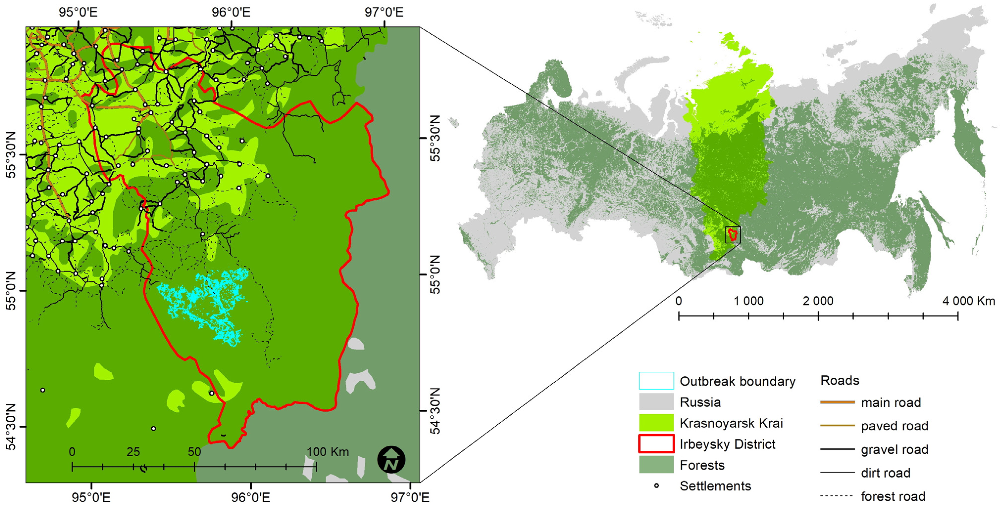
2.1. Study Area
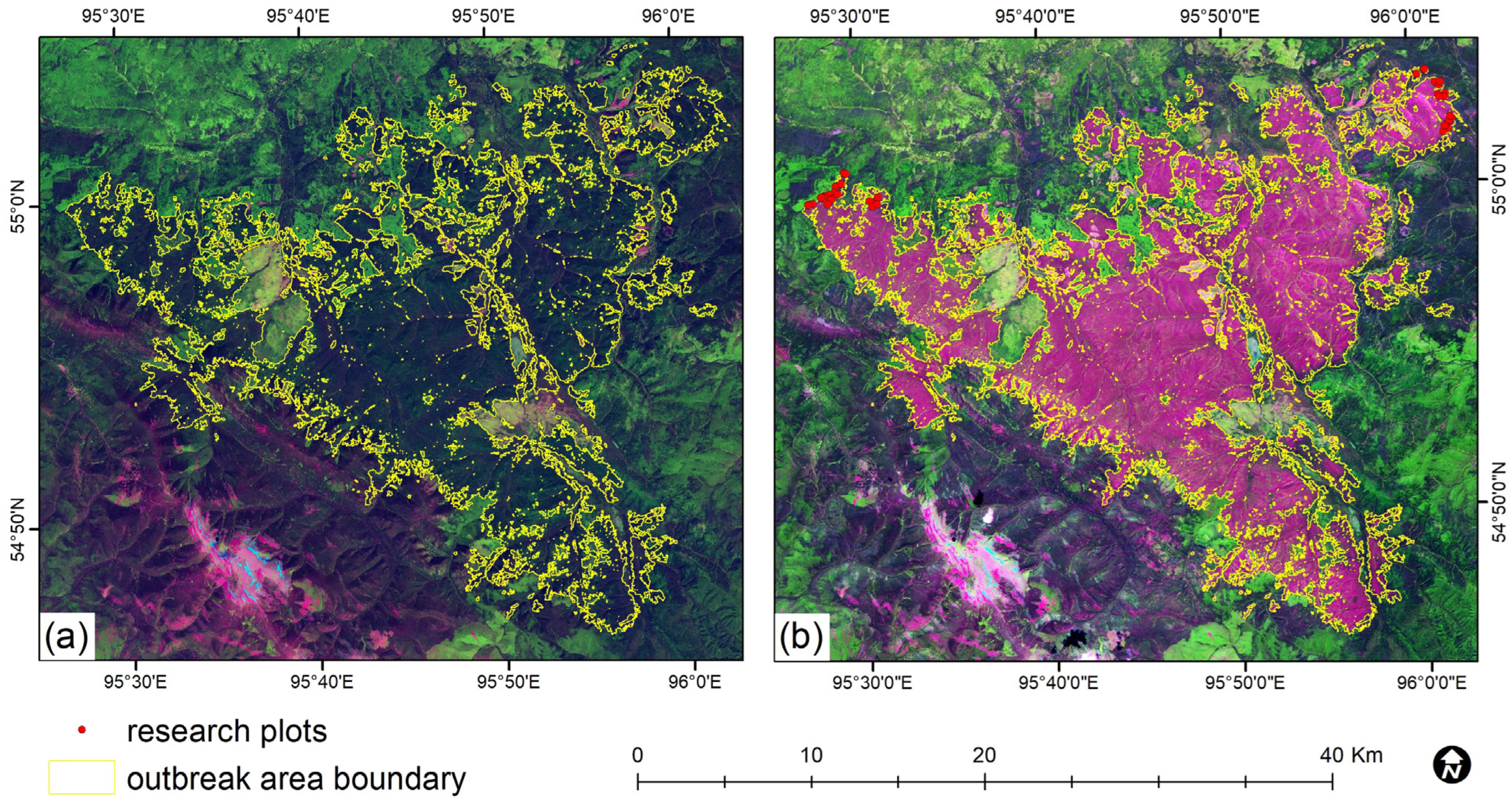
2.2. Field Studies
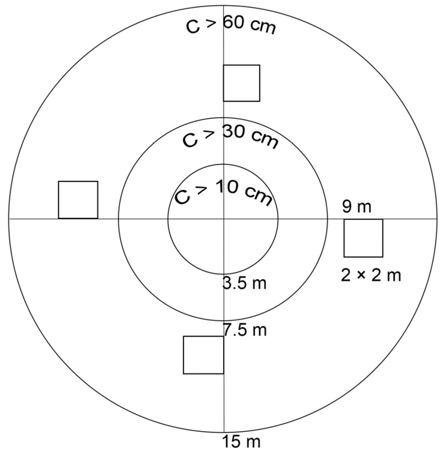
2.2.1. Field Research Methods
2.2.2. Field Data
2.3. Remote Sensing Data
2.4. Methods
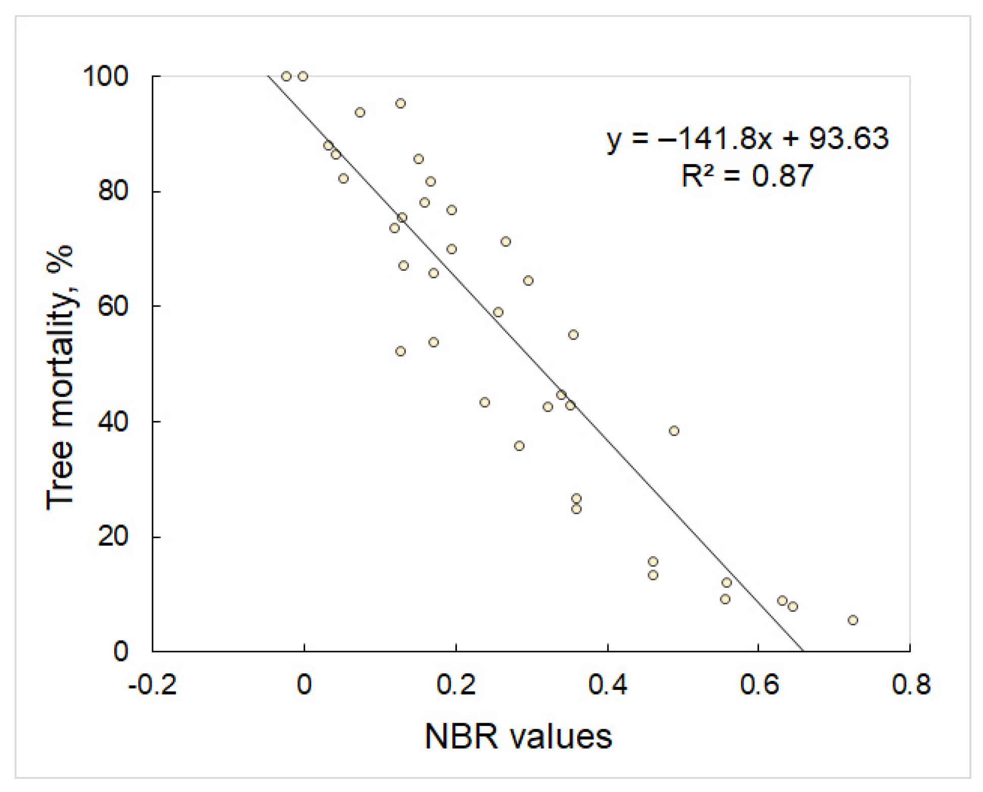
3. Results
4. Discussion
5. Conclusions
Author Contributions
Funding
Data Availability Statement
Acknowledgments
Conflicts of Interest
References
- Gauthier, S.; Bernier, P.; Kuuluvainen, T.; Shvidenko, A.Z.; Schepaschenko, D.G. Boreal forest health and global change. Science 2015, 349, 819–822. [Google Scholar] [CrossRef] [PubMed]
- Dixon, R.K.; Brown, S.; Houghton, R.A.; Solomon, A.M.; Trexler, M.C.; Wisniewski, J. Carbon Pools and Flux of Global Forest Ecosystems. Science 1994, 263, 185–190. [Google Scholar] [CrossRef]
- Masson-Delmotte, V.; Zhai, P.; Pirani, A.; Connors, S.L.; Péan, C.; Berger, S.; Caud, N.; Chen, Y.; Goldfarb, L.; Gomis, M.I. Contribution of Working Group I to the Sixth Assessment Report of the Intergovernmental Panel on Climate Change. In Climate Change 2021: The Physical Science Basis; Cambridge University Press: Cambridge, UK; New York, NY, USA, 2021. [Google Scholar] [CrossRef]
- Flannigan, M.D.; Logan, K.A.; Amiro, B.D.; Skinner, W.R.; Stocks, B.J. Future Area Burned in Canada. Clim. Chang. 2005, 72, 1–16. [Google Scholar] [CrossRef]
- Williams, N.G.; Lucash, M.S.; Ouellette, M.R.; Brussel, T.; Gustafson, E.; Weiss, S.A.; Sturtevant, B.R.; Shchepashchenko, D.; Shvidenko, A. Simulating dynamic fire regime and vegetation change in a warming Siberia. Fire Ecol. 2023, 19, 33. [Google Scholar] [CrossRef]
- Kurz, W.A.; Stinson, G.; Rampley, G.J.; Dymond, C.C.; Neilson, E.T. Risk of natural disturbances makes future contribution of Canada’s forests to the global carbon cycle highly uncertain. Proc. Natl. Acad. Sci. USA 2008, 105, 1551–1555. [Google Scholar] [CrossRef] [PubMed]
- Boldaruev, V.O. Results and prospects for the study and extermination of the Siberian silkmoth in Eastern Siberia. In Materials on the Problem of the Siberian silkmoth; Publishing House of Siberian Brach of USSR Academy of Science: Novosibirsk, Russia, 1960; pp. 3–10. [Google Scholar]
- Galkin, G.I. Some issues of the formation of reservations and primary outbreak spots of the Siberian silkmoth in Krasnoyarsk Krai forests. In Siberian Silkmoth; Publishing House of Siberian Brach of USSR Academy of Science: Novosibirsk, Russia, 1960; pp. 21–33. [Google Scholar]
- Kharuk, V.I.; Antamoshkina, O.A. Impact of Silkmoth Outbreak on Taiga Wildfires. Contemp. Probl. Ecol. 2017, 10, 556–562. [Google Scholar] [CrossRef]
- Fajvan, M.A.; Wood, J.M. Stand structure and development after gypsy moth defoliation in the Appalachian Plateau. For. Ecol. Manag. 1996, 89, 79–88. [Google Scholar] [CrossRef]
- Janes, J.K.; Li, Y.; Keeling, C.I.; Yuen, M.M.S.; Boone, C.K.; Cooke, J.E.K.; Bohlmann, J.; Huber, D.P.W.; Murray, B.W.; Coltman, D.W.; et al. How the mountain pine beetle (Dendroctonus ponderosae) breached the canadian rocky mountains. Mol. Biol. Evol. 2014, 31, 1803–1815. [Google Scholar] [CrossRef]
- Quirion, B.R.; Domke, G.M.; Walters, B.F.; Lovett, G.M.; Fargione, J.E.; Greenwood, L.; Serbesoff-King, K.; Randall, J.M.; Fei, S. Insect and Disease Disturbances Correlate With Reduced Carbon Sequestration in Forests of the Contiguous United States. Front. For. Glob. Chang. 2021, 4, 716582. [Google Scholar] [CrossRef]
- Lehmann, P.; Ammunét, T.; Barton, M.; Battisti, A.; Eigenbrode, S.D.; Jepsen, J.U.; Kalinkat, G.; Neuvonen, S.; Niemelä, P.; Terblanche, J.S.; et al. Complex responses of global insect pests to climate warming. Front. Ecol. Environ. 2020, 18, 141–150. [Google Scholar] [CrossRef]
- Kharuk, V.I.; Im, S.T.; Yagunov, M.N. Migration of the Northern Boundary of the Siberian Silk Moth. Contemp. Probl. Ecol. 2018, 11, 26–34. [Google Scholar] [CrossRef]
- Anderegg, W.R.L.; Hicke, J.A.; Fisher, R.A.; Allen, C.D.; Aukema, J.; Bentz, B.; Hood, S.; Lichstein, J.W.; Macalady, A.K.; Mcdowell, N.; et al. Tree mortality from drought, insects, and their interactions in a changing climate. New Phytol. 2015, 208, 674–683. [Google Scholar] [CrossRef] [PubMed]
- Kondakov, Y.P. The outbreaks of Siberian silk moth in Krasnoyarsk krai forests. In Entomological Researches in Siberia; KF RES: Krasnoyarsk, Russia, 2002; Volume 2, pp. 25–74. [Google Scholar]
- Epova, V.I.; Pleshanov, A.S. Zones of Severity of Phyllophagous Insects in Asian Russia; Nauka, Siberian Publishing House RAS: Novosibirsk, Russia, 1995; p. 47. [Google Scholar]
- Kolomiets, N.G. Siberian silkworm—A pest of the lowland taiga. In Proceedings on Forestry of Western Siberia; Nauka: Novosibirsk, Russia, 1957; Volume 3, pp. 61–76. [Google Scholar]
- Kondakov, Y.P. Mass reproduction of Siberian silk moth. In Ekologiya Populyatsii Lesnykh Zhivotnykh Sibiri (Population Ecology of Forest Animals in Siberia); Nauka: Novosibirsk, Russia, 1974; pp. 206–264. [Google Scholar]
- Grodnitsky, D.L. Siberian silkworm and the fate of fir taiga. Nature 2004, 11, 49–56. [Google Scholar]
- Pavlov, I.N.; Litovka, Y.A.; Golubev, D.V.; Astapenko, S.A.; Chromogin, P.V. New outbreak of Dendrolimus sibiricus tschetv. in Siberia (2012–2017): Monitoring, modeling and biological control. Contemp. Probl. Ecol. 2018, 11, 406–419. [Google Scholar] [CrossRef]
- Furyaev, V.V. Forests That Died after Siberian Silk Moth Outbreaks and Thier Prescribed Burning; Nauka: Moskow, Russia, 1966. [Google Scholar]
- Isaev, A.S.; Palnikova, E.N.; Sukhovolsky, V.G.; Tarasova, O.V. Population Dynamics of Defoliating Forest Insects: Models and Forecasts; KMK Scientific Press Ltd.: Moscow, Russia, 2015; p. 262. [Google Scholar]
- Isaev, A.S.; Soukhovolsky, V.G.; Tarasova, O.V.; Palnikova, E.N.; Kovalev, A.V. Forest Insect Population Dynamics, Outbreaks and Global Warming Effects; Wiley: Hoboken, NJ, USA, 2017; 298p. [Google Scholar]
- Soukhovolsky, V.G.; Kovalev, A.V.; Palnikova, E.N.; Tarasova, O.V. Modelling the risk of insect impacts on forest stands after possible climate changes. Comput. Stud. Model. 2016, 8, 241–253. [Google Scholar] [CrossRef]
- Demidko, D.A.; Goroshko, A.A.; Slinkina, O.A.; Mikhaylov, P.V.; Sultson, S.M. The Role of Forest Stands Characteristics on Formation of Exterior Migratory Outbreak Spots by the Siberian Silk Moth Dendrolimus sibiricus (Tschetv.) during Population Collapse. Forests 2023, 14, 1078. [Google Scholar] [CrossRef]
- Franklin, J.F.; Lindenmayer, D.B.; MacMahon, J.A.; McKee, A.; Magnusson, J.; Perry, D.A.; Waide, R.; Foster, D. Threads of continuity: Ecosystems disturbances, biological legacies, and ecosystem recovery. Conserv. Biol. Pract. 2000, 1, 8–17. [Google Scholar] [CrossRef]
- Valendik, E.N.; Verkhovets, S.V.; Kisilyakhov, E.K.; Lantukh, A.Y. The role of forests damaged by the Siberian silkmoth in forest fires in the Lower Angara region. For. Manag. 2004, 6, 27–29. [Google Scholar]
- Jonášová, M.; Prach, K. The Influence of Bark Beetles Outbreak vs. Salvage Logging on Ground Layer Vegetation in Central European Mountain Spruce Forests. Biol. Conserv. 2008, 141, 1525–1535. [Google Scholar] [CrossRef]
- Niemelä, J. Management in Relation to Disturbance in the Boreal Forest. For. Ecol. Manag. 1999, 115, 127–134. [Google Scholar] [CrossRef]
- Davis, S.M.; Landgrebe, D.A.; Phillips, T.L.; Swain, P.H.; Hoffer, R.M.; Lindenlaub, J.C.; Silva, L.F. Remote Sensing: The Quantitative Approach; McGraw-Hill International Book Co.: New York, NY, USA, 1978. [Google Scholar]
- Vygodskaya, I.N.; Gorshkova, I.I. Theory and Experiment in Remote-Sensing Studies of Vegetation; Gidrometeoizdat: Moscow, Russia, 1987; p. 246. [Google Scholar]
- Kronberg, P. Remote-Sensing Study of the Earth; Mir: Moscow, Russia, 1988; p. 350. [Google Scholar]
- Senf, C.; Seidl, R.; Hostert, P. Remote sensing of forest insect disturbances: Current state and future directions. Int. J. Appl. Earth Obs. Geoinform. 2017, 60, 49–60. [Google Scholar] [CrossRef] [PubMed]
- Meng, R.; Gao, R.; Zhao, F.; Huang, C.; Sun, R.; Lv, Z.; Huang, Z. Landsat-based monitoring of southern pine beetle infestation severity and severity change in a temperate mixed forest. Remote Sens. Environ. 2022, 269, 112847. [Google Scholar] [CrossRef]
- Long, J.; Lawrence, R. Mapping Percent Tree Mortality Due to Mountain Pine Beetle Damage. For. Sci. 2016, 62, 392–402. [Google Scholar] [CrossRef]
- Havašová, M.; Bucha, T.; Ferenčík, J.; Jakuš, R. Applicability of a vegetation indices-based method to map bark beetle outbreaks in the High Tatra Mountains. Ann. For. Res. 2015, 58, 295–310. [Google Scholar] [CrossRef]
- Meddens, A.J.H.; Hicke, J.A.; Vierling, L.A.; Hudak, A.T. Evaluating methods to detect bark beetle-caused tree mortality using single-date and multi-date Landsat imagery. Remote Sens. Environ. 2013, 132, 49–58. [Google Scholar] [CrossRef]
- Meigs, G.W.; Kennedy, R.E.; Cohen, W.B. A Landsat time series approach to characterize bark beetle and defoliator impacts on tree mortality and surface fuels in conifer forests. Remote Sens. Environ. 2011, 115, 3707–3718. [Google Scholar] [CrossRef]
- Hart, S.J.; Veblen, T.T. Detection of Spruce Beetle-Induced Tree Mortality Using High- and Medium-Resolution Remotely Sensed Imagery. Remote Sens. Environ. 2015, 168, 134–145. [Google Scholar] [CrossRef]
- Kharuk, V.I.; Ranson, K.J.; Kozuhovskaya, A.G.; Kondakov, Y.P.; Pestunov, I.A. NOAA/AVHRR satellite detection of Siberian silkmoth outbreaks in eastern Siberia. Int. J. Remote Sens. 2004, 25, 5543–5555. [Google Scholar] [CrossRef]
- Ershov, D.V.; Devyatova, N.V. Application of satellite survey data to monitor mass outbreaks of Siberian moth. Izv. Vyssh. Uchebn. Zaved. Geod. Aerofotos’emka 2008, 2, 161–167. [Google Scholar]
- Fassnacht, F.E.; Latifi, H.; Ghosh, A.; Joshi, P.K.; Koch, B. Assessing the potential of hyperspectral imagery to map bark beetle-induced tree mortality. Remote Sens. Environ. 2014, 140, 533–548. [Google Scholar] [CrossRef]
- Hicke, J.A.; Logan, J. Mapping whitebark pine mortality caused by a mountain pine beetle outbreak with high spatial resolution satellite imagery. Int. J. Remote Sens. 2009, 30, 4427–4441. [Google Scholar] [CrossRef]
- Coops, N.C.; Johnson, M.; Wulder, M.A.; White, J.C. Assessment of QuickBird high spatial resolution imagery to detect red attack damage due to mountain pine beetle infestation. Remote Sens. Environ. 2006, 103, 67–80. [Google Scholar] [CrossRef]
- Smagin, V.N.; Ilinskaya, S.A.; Nazimova, D.I.; Novoseltseva, I.F.; Cherednikova, J.S. Forest Types of Mountains of Southern Siberia; Nauka: Novosibirsk, Russia, 1980; p. 336. [Google Scholar]
- Polikarpov, N.P.; Chebakova, N.M.; Nazimova, D.I. Climate and Mountain Forests in Southern Siberia; Nauka: Novosibirsk, Russia, 1986; p. 225. [Google Scholar]
- Order of Federal Forestry Agency on Approval of the Regulations for Organizing and Carrying Out Activities for State Forest Inventory; Federal Forestry Agency, Its Territorial Authorities and Subordinate Organizations: Moscow, Russia, 2022.
- Zhuravlev, P.G. Recommendations for Siberian Silkworm Control in the Forests of Russian Far East; FEFRI: Khabarovsk, Russia, 1960; p. 33. [Google Scholar]
- Grodnitsky, D.L.; Raznobarsky, V.G.; Soldatov, V.V.; Remarchuk, N.P. Degradation of taiga forests disturbed by the Siberian silkmoth. Contemp. Probl. Ecol. 2002, 1, 3–12. [Google Scholar]
- Baranchikov, Y.N.; Perevoznikova, V.D. The Siberian silkmoth outbreak areas as a source of additional carbon emissions. In Readings in Memory of Academician V. N. Sukachev. XX. Insects in Forest Biogeocenoses; KMK Scientific Press Ltd. Publishing House: Moscow, Russia, 2004; pp. 32–53. [Google Scholar]
- Krivolutskaya, G.O. Secretive Stem Pests in Dark Coniferous Forests Damaged by the Siberian Silkmoth in Western Siberia; Nauka: Moscow, Russia, 1965; p. 130. [Google Scholar]
- Forest Cover Loss Map from Global Forest Watch Dataset v1.10. Available online: https://data.globalforestwatch.org/ (accessed on 2 September 2023).
- Hansen, M.C.; Potapov, P.V.; Moore, R.; Hancher, M.; Turubanova, S.A.; Tyukavina, A.; Thau, D.; Stehman, S.V.; Goetz, S.J.; Loveland, T.R.; et al. High-Resolution Global Maps of 21st-Century Forest Cover Change. Science 2013, 342, 850–853. [Google Scholar] [CrossRef] [PubMed]
- Giglio, L.; Boschetti, L.; Roy, D.P.; Humber, M.L.; Justice, C.O. The Collection 6 MODIS burned area mapping algorithm and product. Remote Sens. Environ. 2018, 217, 72–85. [Google Scholar] [CrossRef]
- USGS Earthexplorer. Available online: https://earthexplorer.usgs.gov/ (accessed on 14 August 2023).
- Copernicus Open Access Hub. Available online: https://scihub.copernicus.eu (accessed on 2 September 2023).
- Sentinel Online. Sentinel-2 Annual Performance Report—Year 2022. Available online: https://sentinels.copernicus.eu/ca/web/sentinel/user-guides/sentinel-2-msi/document-library (accessed on 21 September 2023).
- Tucker, C.J. Red and photographic infrared linear combinations for monitoring vegetation. Remote Sens. Environ. 1979, 8, 127–150. [Google Scholar] [CrossRef]
- Zhu, Z.; Key, C.H.; Ohlen, D.; Benson, N.C. Evaluate Sensitivities of Burn-Severity Mapping Algorithms for Different Ecosystems and Fire Histories in the United States; Final Report to the Joint Fire Sciences Program, JFSP 01-1-4-12; Joint Fire Science Program: Boise, IA, USA, 2006.
- Key, C.H.; Benson, N.; Ohlen, D.; Howard, S.; McKinley, R.; Zhu, Z. The normalized burn ratio and relationships to burn severity: Ecology, remote sensing and implementation. In Proceedings of the Ninth Forest Service Remote Sensing Applications Conference, San Diego, CA, USA, 8–12 April 2002; Greer, J.D., Ed.; American Society for Photogrammetry and Remote Sensing: Bethesda, MD, USA, 2002. [Google Scholar]
- Key, C.H. Ecological and sampling constraints on defining landscape fire severity. Fire Ecol. 2006, 2, 34–59. [Google Scholar] [CrossRef]
- Gao, B.-C. NDWI—A normalized difference water index for remote sensing of vegetation liquid water fromspace. Remote Sens. Environ. 1996, 58, 257–266. [Google Scholar] [CrossRef]
- Gao, X.; Huete, A.R.; Ni, W.; Miura, T. Optical–biophysical relationships of vegetation spectra without background contamination. Remote Sens. Environ. 2000, 74, 609–620. [Google Scholar] [CrossRef]
- Crist, E.P.; Cicone, R.C. A physically-based transformation of Thematic Mapper data—The TM Tasseled Cap. IEEE Trans. Geosci. Remote Sens. 1984, 22, 256–263. [Google Scholar] [CrossRef]
- Kuhn, M. Building Predictive Models in R Using the caret Package. J. Stat. Softw. 2008, 28, 1–26. [Google Scholar] [CrossRef]
- Gareth, J.; Witten, D.; Hastie, T.; Tibshirani, R. An Introduction to Statistical Learning: With Applications in R; Springer Publishing Company, Incorporated: New York, NY, USA, 2014. [Google Scholar] [CrossRef]
- Pasquarella, V.J.; Bradley, B.A.; Woodcock, C.E. Near-Real-Time Monitoring of Insect Defoliation Using Landsat Time Series. Forests 2017, 8, 275. [Google Scholar] [CrossRef]
- Rahimzadeh-Bajgiran, P.; Weiskittel, A.R.; Kneeshaw, D.; MacLean, D.A. Detection of Annual Spruce Budworm Defoliation and Severity Classification Using Landsat Imagery. Forests 2018, 9, 357. [Google Scholar] [CrossRef]
- Townsend, P.A.; Singh, A.; Foster, J.R.; Rehberg, N.J.; Kingdon, C.C.; Eshleman, K.N.; Seagle, S.W. A general Landsat model to predict canopy defoliation in broadleaf deciduous forests. Remote Sens. Environ. 2012, 119, 255–265. [Google Scholar] [CrossRef]
- De Beurs, K.M.; Townsend, P.A. Estimating the effect of gypsy moth defoliation using MODIS. Remote Sens. Environ. 2008, 112, 3983–3990. [Google Scholar] [CrossRef]
- Fraser, R.H.; Latifovic, R. Mapping insect-induced tree defoliation and mortality using coarse spatial resolution satellite imagery. Int. J. Remote Sens. 2005, 26, 193–200. [Google Scholar] [CrossRef]

| Band/Spectral Range | Sentinel-2A | Sentinel-2B | Spatial Resolution (m) |
|---|---|---|---|
| Central Wavelength (nm) | |||
| 1/ Coastal Aerosol (COASTAL BLUE) | 422.7 | 422.3 | 60 |
| 2/ Visible Blue (BLUE) | 492.7 | 492.3 | 10 |
| 3/ Visible Green (GREEN) | 559.8 | 558.9 | 10 |
| 4/ Visible Red (RED) | 664.6 | 664.9 | 10 |
| 5/ Vegetation Read Edge (RE1) | 704.1 | 703.8 | 20 |
| 6/ Vegetation Read Edge (RE2) | 740.5 | 739.1 | 20 |
| 7/ Vegetation Read Edge (RE3) | 782.8 | 779.7 | 20 |
| 8/ Near Infrared (NIR) | 832.8 | 832.9 | 10 |
| 8a/ Narrow Near-Infrared (RE4) | 864.7 | 864 | 20 |
| 9/ Water Vapor | 945.1 | 943.2 | 60 |
| 10/ Cirrus Short Wave Infrared (SWIR) | 1373.5 | 1376.9 | 60 |
| 11/ Short Wave Infrared (SWIR1) | 1613.7 | 1610.4 | 20 |
| 12/ Short Wave Infrared (SWIR2) | 2202.4 | 2185.7 | 20 |
| Scene ID | Scene Date | Satellite |
|---|---|---|
| S2A_MSIL2A_20180625T045701_N9999_R119_T46UFF/T46UFG | 25 June 2018 | Sentinel 2A |
| S2A_MSIL2A_20200810T044711_N0214_R076_T46UFF/T46UFG | 10 August 2020 | Sentinel 2A |
| S2A_MSIL2A_20200922T045701_N0214_R119_T46UFF/T46UFG | 22 September 2020 | Sentinel 2A |
| S2B_MSIL1C_20210601T044659_N0300_R076_T46UFF/T46UFG | 1 June 2021 | Sentinel 2B |
| S2B_MSIL2A_20210704T045659_N0301_R119_T46UFF/T46UFG | 4 July 2021 | Sentinel 2B |
| S2A_MSIL2A_20210828T045701_N0301_R119_T46UFF/T46UFG | 28 August 2021 | Sentinel 2A |
| S2A_MSIL2A_20211017T045811_N0500_R119_T46UFF/T46UFG | 17 October 2021 | Sentinel 2A |
| S2A_MSIL1C_20220512T044701_N0400_R076_T46UFF/T46UFG | 12 May 2022 | Sentinel 2A |
| S2A_MSIL1C_20220611T044711_N0400_R076_T46UFF/T46UFG | 11 June 2022 | Sentinel 2A |
| S2B_MSIL2A_20220808T045659_N0400_R119_ T46UFF/T46UFG | 8 August 2022 | Sentinel 2B |
| S2A_MSIL2A_20220919T044711_N0400_R076_ T46UFF/T46UFG | 19 September 2022 | Sentinel 2A |
| S2A_MSIL1C_20230616T044701_N0509_R076_T46UFF/T46UFG | 16 June 2023 | Sentinel 2A |
| S2A_MSIL1C_20230825T044701_N0509_R076_T46UFF/T46UFG | 25 August 2023 | Sentinel 2A |
| Index | Formula | Reference |
|---|---|---|
| NDVI (Normalized Difference Vegetation Index) | (NIR − RED)/(NIR + RED) | Tucker, 1979 [59] |
| dNDVI (difference in Normalized Difference Vegetation Index) | NDVIpre − NDVIpost | Zhu et al., 2006 [60] |
| NBR (Normalized Burn Ratio) | (NIR − SWIR2)/(NIR + SWIR2) | Key et al., 2002 [61] |
| dNBR (difference in Normalized Burn Ratio) | NBRpre − NBRpost | Key, 2006 [62] |
| NDMI (Normalized Difference Moisture Index) | (NIR − SWIR1)/(NIR + SWIR1) | Gao, 1996 [63] |
| EVI (Enhanced Vegetation Index) | 2.5(NIR − RED)/(NIR + 6RED − 7.5BLUE) + 1 | Gao et al., 2000 [64] |
| TCG (Tasseled Cap Greenness) | −0.28482BLUE − 0.24353GREEN − 0.54364RED + 0.72438NIR + 0.084011SWIR1 − 0.180012SWIR2 | Crist et al., 1984 [65] |
| Date | Accuracy | |||||||
|---|---|---|---|---|---|---|---|---|
| NDVI | dNDVI | NBR | dNBR | NDMI | EVI | TCG | ||
| 10 August 2020 | R2 | 0.623 | 0.662 | 0.749 | 0.712 | 0.710 | 0.584 | 0.564 |
| RMSE | 17.962 | 17.663 | 15.775 | 15.908 | 15.605 | 20.888 | 20.268 | |
| MAE | 15.500 | 15.081 | 13.597 | 13.833 | 13.287 | 17.835 | 17.177 | |
| 22 September 2020 | R2 | 0.820 | 0.848 | 0.872 | 0.855 | 0.866 | 0.826 | 0.839 |
| RMSE | 13.126 | 12.936 | 11.427 | 11.897 | 11.572 | 15.018 | 14.871 | |
| MAE | 11.258 | 10.876 | 9.602 | 10.524 | 9.949 | 12.016 | 11.920 | |
| 1 June 2021 | R2 | 0.539 | 0.624 | 0.670 | 0.715 | 0.635 | 0.504 | 0.558 |
| RMSE | 20.609 | 19.451 | 18.161 | 16.891 | 18.455 | 21.759 | 21.040 | |
| MAE | 17.260 | 16.083 | 15.807 | 14.846 | 16.077 | 18.939 | 18.054 | |
| 4 July 2021 | R2 | 0.635 | 0.614 | 0.699 | 0.715 | 0.635 | 0.340 * | 0.325 * |
| RMSE | 19.930 | 19.058 | 16.995 | 16.891 | 18.455 | 25.820 | 25.263 | |
| MAE | 16.896 | 16.366 | 14.982 | 14.846 | 16.077 | 22.401 | 22.088 | |
| 28 August 2021 | R2 | 0.742 | 0.769 | 0.851 | 0.840 | 0.841 | 0.696 | 0.669 |
| RMSE | 15.442 | 14.506 | 12.490 | 12.455 | 12.530 | 18.566 | 17.703 | |
| MAE | 12.531 | 11.892 | 10.452 | 10.700 | 10.331 | 14.875 | 14.157 | |
| 17 October 2021 | R2 | 0.712 | 0.703 | 0.626 | 0.581 | 0.603 | 0.695 | 0.699 |
| RMSE | 16.732 | 15.855 | 18.909 | 20.121 | 20.300 | 17.944 | 17.115 | |
| MAE | 14.059 | 12.688 | 16.706 | 16.933 | 17.140 | 15.155 | 14.747 | |
| 12 May 2022 | R2 | 0.703 | 0.692 | 0.790 | 0.797 | 0.796 | 0.722 | 0.733 |
| RMSE | 17.335 | 17.088 | 14.223 | 13.533 | 14.445 | 16.322 | 15.799 | |
| MAE | 14.310 | 13.748 | 11.973 | 11.316 | 12.117 | 13.216 | 12.784 | |
| 11 June 2022 | R2 | 0.750 | 0.768 | 0.766 | 0.773 | 0.716 | 0.509 | 0.500 |
| RMSE | 15.376 | 14.883 | 15.181 | 14.872 | 15.732 | 22.107 | 21.781 | |
| MAE | 12.439 | 11.805 | 12.691 | 12.814 | 12.953 | 18.021 | 17.904 | |
| 8 August 2022 | R2 | 0.791 | 0.779 | 0.809 | 0.768 | 0.809 | 0.627 | 0.661 |
| RMSE | 14.486 | 14.044 | 13.866 | 14.419 | 13.456 | 19.329 | 19.157 | |
| MAE | 11.711 | 11.091 | 11.796 | 12.494 | 11.492 | 15.723 | 15.362 | |
| 19 September 2022 | R2 | 0.721 | 0.720 | 0.847 | 0.849 | 0.851 | 0.761 | 0.774 |
| RMSE | 15.823 | 15.668 | 12.412 | 12.507 | 12.137 | 14.683 | 15.056 | |
| MAE | 12.465 | 12.354 | 10.134 | 10.502 | 9.629 | 11.539 | 11.971 | |
| 16 June 2023 | R2 | 0.697 | 0.690 | 0.693 | 0.665 | 0.720 | 0.417 | 0.443 |
| RMSE | 17.324 | 17.391 | 17.275 | 17.809 | 16.762 | 24.659 | 23.888 | |
| MAE | 13.906 | 13.694 | 14.810 | 15.484 | 14.201 | 21.249 | 20.526 | |
| 25 August 2023 | R2 | 0.704 | 0.710 | 0.802 | 0.791 | 0.800 | 0.554 | 0.583 |
| RMSE | 16.461 | 16.802 | 13.152 | 13.751 | 13.649 | 21.135 | 20.672 | |
| MAE | 13.483 | 13.801 | 10.302 | 11.483 | 10.569 | 16.454 | 16.027 | |
Disclaimer/Publisher’s Note: The statements, opinions and data contained in all publications are solely those of the individual author(s) and contributor(s) and not of MDPI and/or the editor(s). MDPI and/or the editor(s) disclaim responsibility for any injury to people or property resulting from any ideas, methods, instructions or products referred to in the content. |
© 2023 by the authors. Licensee MDPI, Basel, Switzerland. This article is an open access article distributed under the terms and conditions of the Creative Commons Attribution (CC BY) license (https://creativecommons.org/licenses/by/4.0/).
Share and Cite
Slinkina, O.A.; Mikhaylov, P.V.; Sultson, S.M.; Demidko, D.A.; Khizhniak, N.P.; Tatarintsev, A.I. Mapping Tree Mortality Caused by Siberian Silkmoth Outbreak Using Sentinel-2 Remote Sensing Data. Forests 2023, 14, 2436. https://doi.org/10.3390/f14122436
Slinkina OA, Mikhaylov PV, Sultson SM, Demidko DA, Khizhniak NP, Tatarintsev AI. Mapping Tree Mortality Caused by Siberian Silkmoth Outbreak Using Sentinel-2 Remote Sensing Data. Forests. 2023; 14(12):2436. https://doi.org/10.3390/f14122436
Chicago/Turabian StyleSlinkina, Olga A., Pavel V. Mikhaylov, Svetlana M. Sultson, Denis A. Demidko, Natalia P. Khizhniak, and Andrey I. Tatarintsev. 2023. "Mapping Tree Mortality Caused by Siberian Silkmoth Outbreak Using Sentinel-2 Remote Sensing Data" Forests 14, no. 12: 2436. https://doi.org/10.3390/f14122436
APA StyleSlinkina, O. A., Mikhaylov, P. V., Sultson, S. M., Demidko, D. A., Khizhniak, N. P., & Tatarintsev, A. I. (2023). Mapping Tree Mortality Caused by Siberian Silkmoth Outbreak Using Sentinel-2 Remote Sensing Data. Forests, 14(12), 2436. https://doi.org/10.3390/f14122436