
Ecological Carrying Capacity Estimation of the Trails in a Protected Area: Integrating a Path Analysis Model and the Stakeholders’ Evaluation


Abstract
:
1. Introduction
2. Method
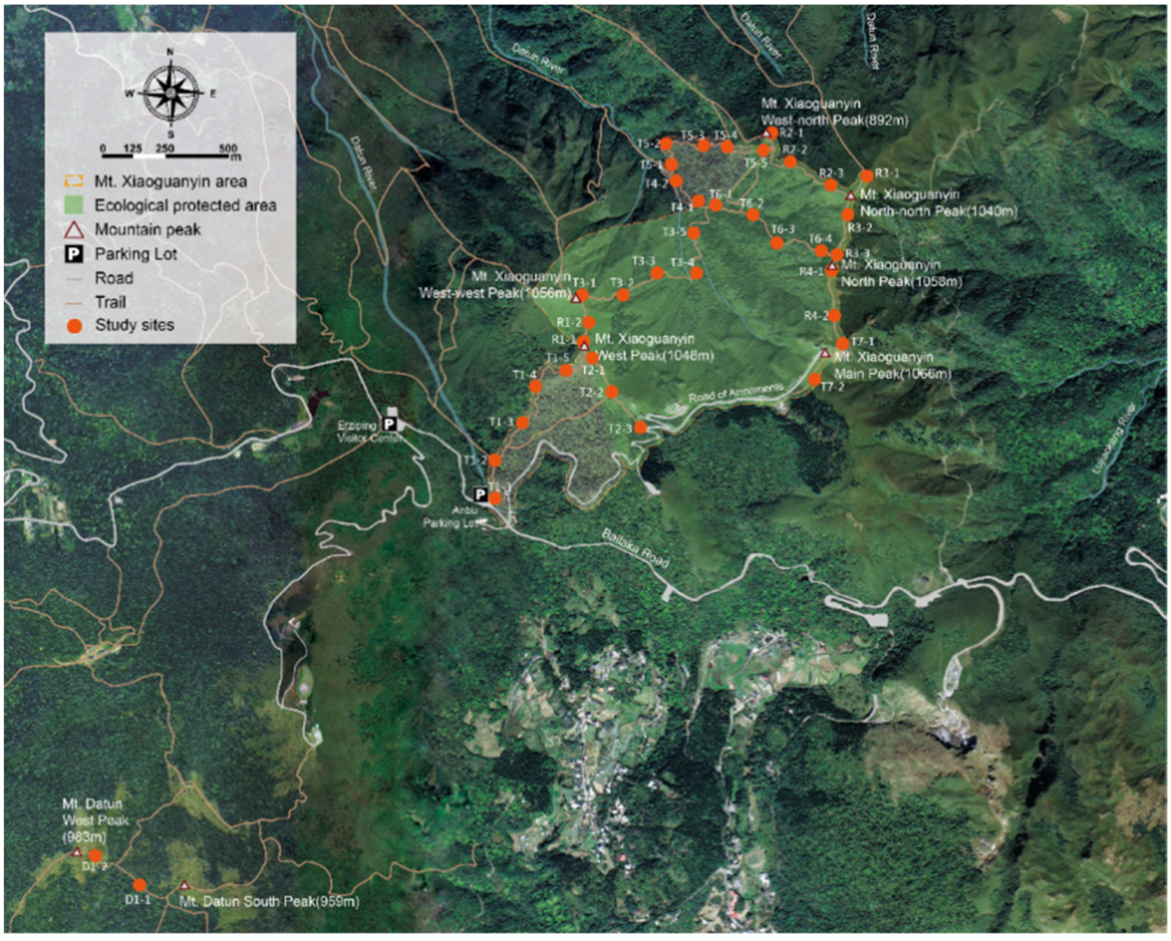
2.1. Study Area
2.2. Use–Impact Model Establishment
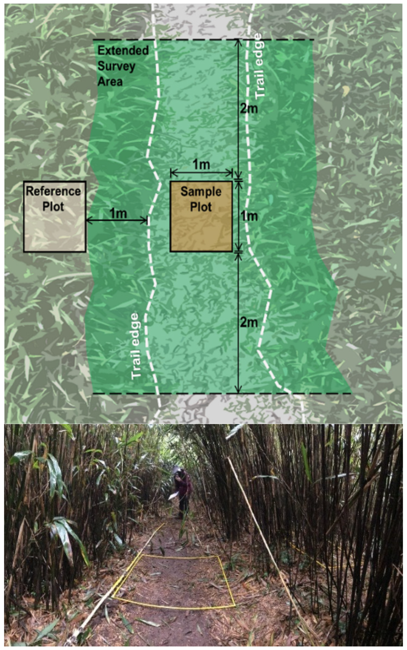
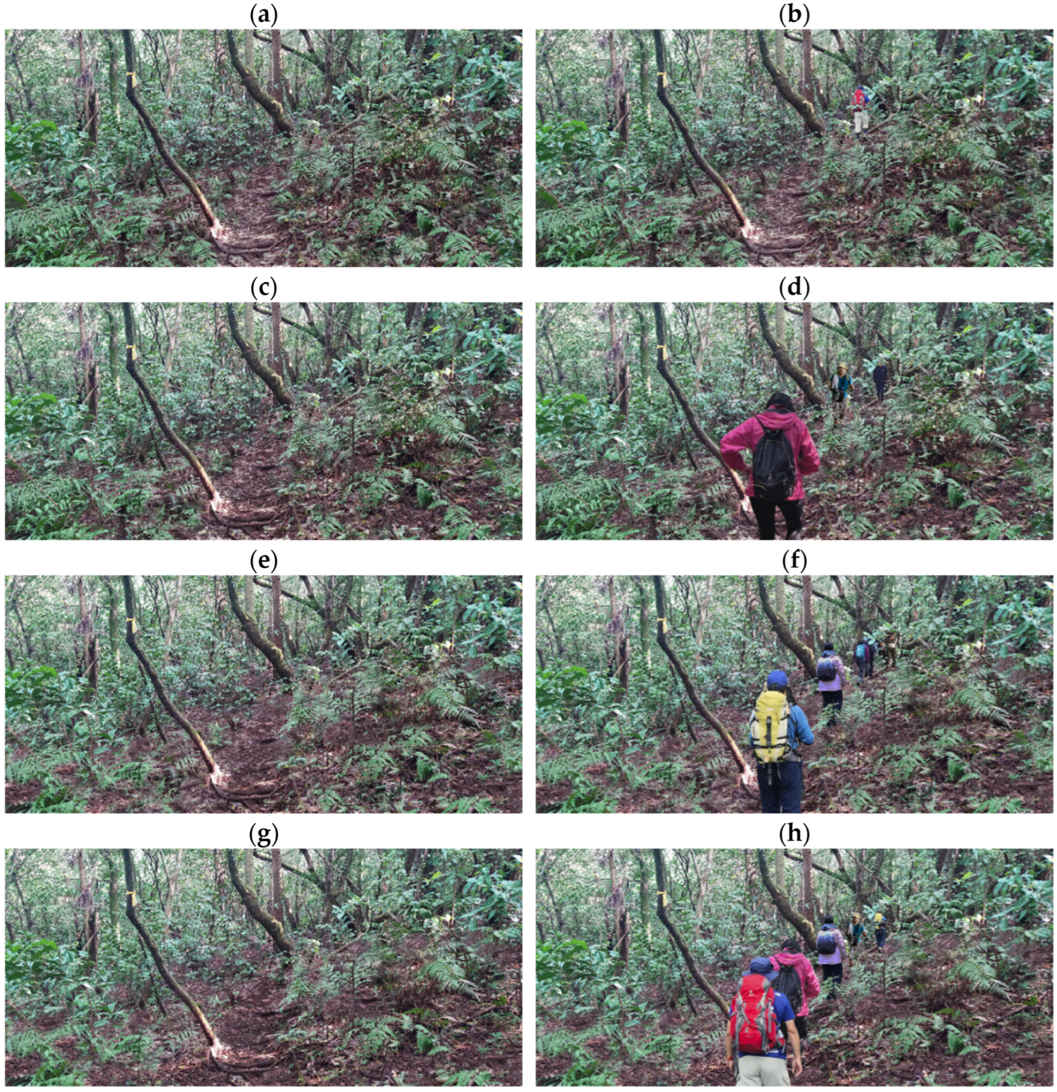
2.2.1. Use–Impact Survey along the Trails
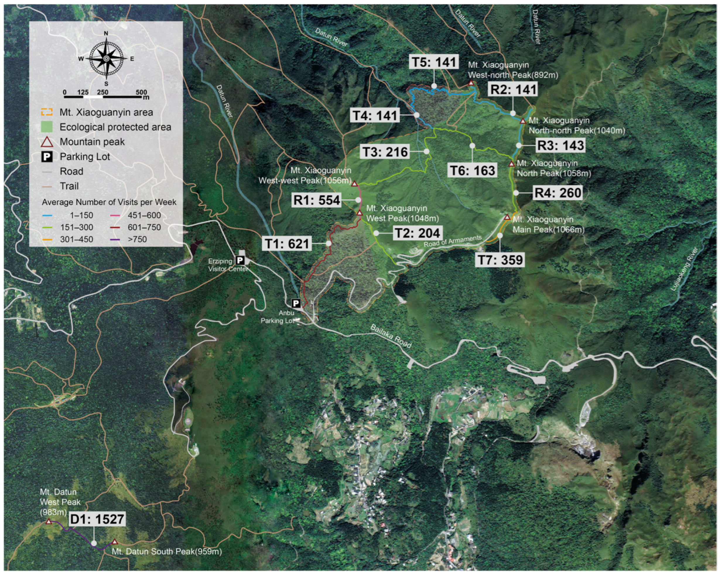
2.2.2. Trail Usage Counting and Estimating
- A.
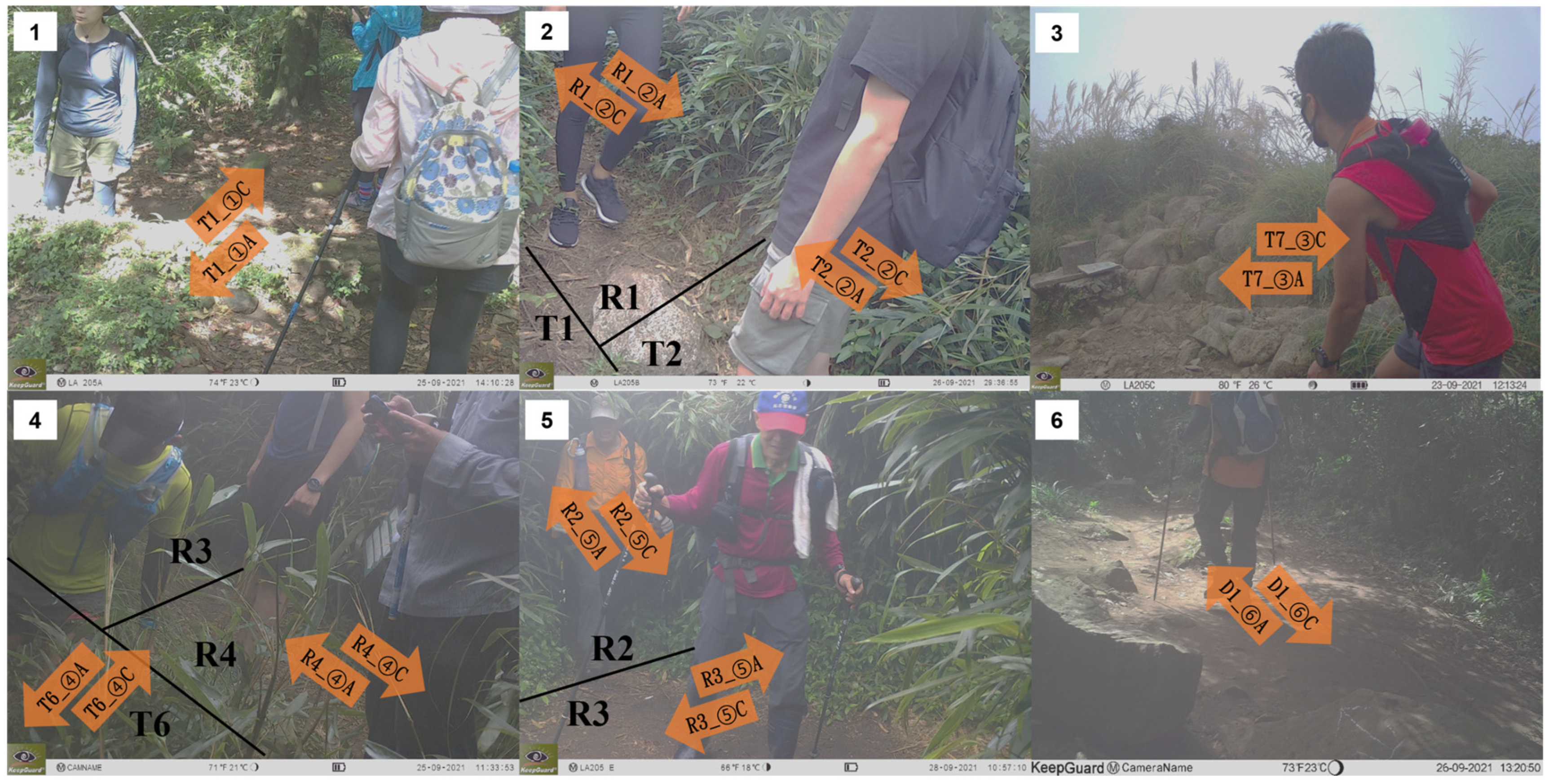
- Infrared trigger camera setting and trail usage
- B.
- Estimation and calibration of the trail peak usage
2.2.3. Conceptual Use–Impact Model
2.3. Stakeholders’ Acceptance Evaluation
2.3.1. Scenarios Simulation
2.3.2. Stakeholder Evaluation Survey
2.3.3. Acceptance Range of Ecological Carrying Capacity
3. Results
3.1. Use–Impact Model
3.1.1. Trail Usage
3.1.2. Landscape-Level Conditions and Use–Impact Factors along the Trails
3.1.3. The Use–Impact Model
- A.
- Relationship between Use and Impact
- B.
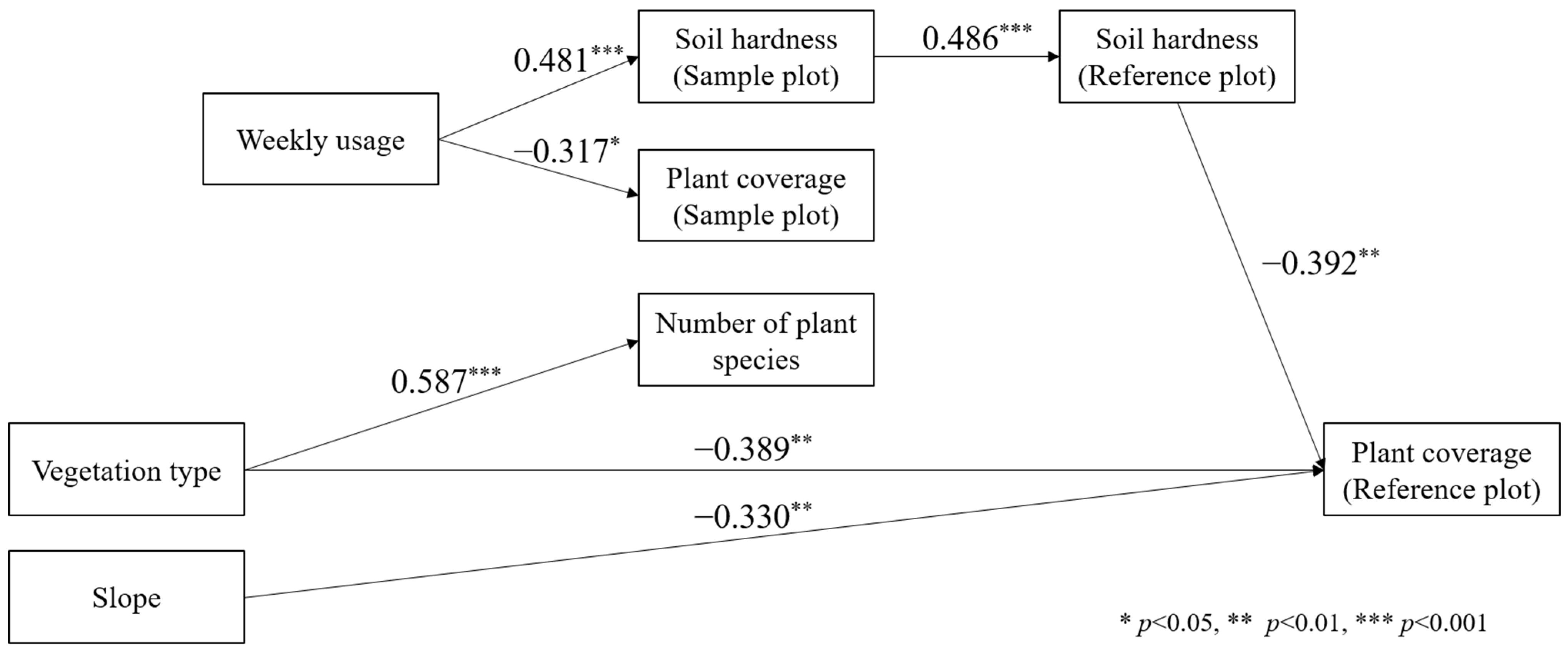
- Path analysis result of the Use–Impact model
3.2. Evaluation of Ecological Carrying Capacity
3.2.1. Simulated Scenarios
- A.
- Scenario 1: increased by 4% with 288 total hikers per week
- B.
- Scenario 2: baseline level with 404 total hikers per week
- C.
- Scenario 3: decreased by 10% with 696 total hikers per week
- D.
- Scenario 4: decreased by 20% with 988 total hikers per week
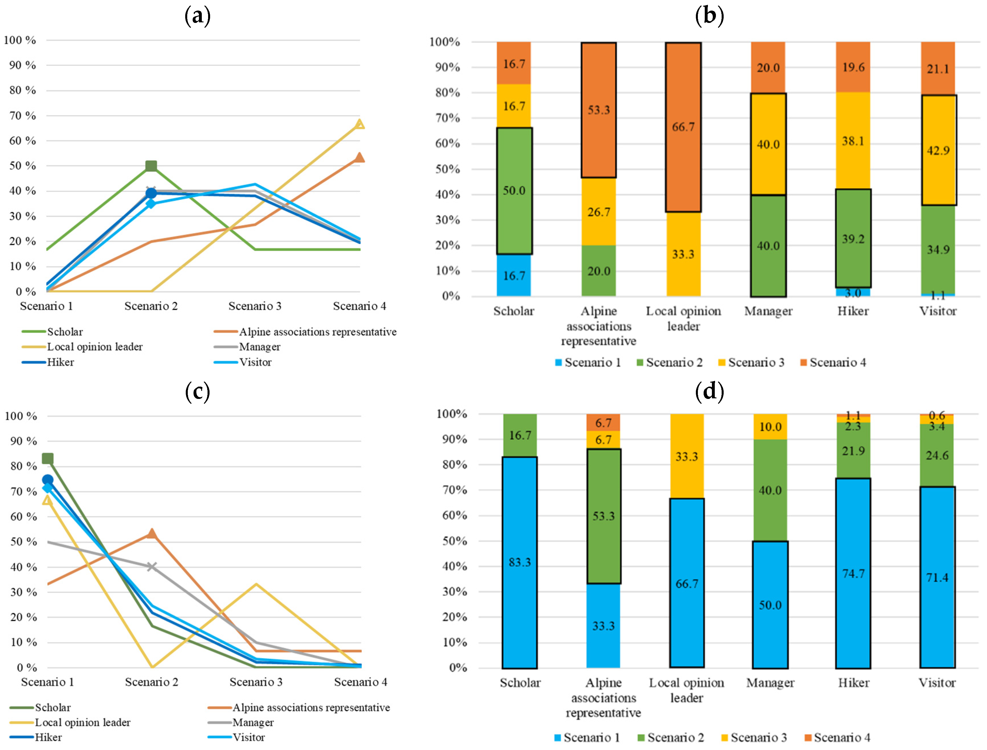
3.2.2. Acceptance Evaluation of the Stakeholders
3.2.3. Acceptance Range of Ecological Carrying Capacity
4. Discussion
4.1. Use–Impact Model
4.1.1. The Affect Paths of the Landscape-Level Conditions and Usage Impacts
4.1.2. Impact Factors and Future Path Model Refinement
4.2. Evaluation of Ecological Carrying Capacity
4.2.1. Objective and Subjective Estimation of Ecological Carrying Capacity
4.2.2. Long-Term Monitoring and Rolling Adjustment
5. Conclusions
Author Contributions
Funding
Data Availability Statement
Conflicts of Interest
References
- Outdoor Foundation 2022. 2022 Outdoor Participation Trends Report. Available online: https://outdoorindustry.org/resource/2022-outdoor-participation-trends-report/ (accessed on 27 September 2022).
- Beery, T.; Olsson, M.R.; Vitestam, M. COVID-19 and outdoor recreation management: Increased participation, connection to nature, and a look to climate adaptation. J. Outdoor Recreat. Tour. 2021, 36, 100457. [Google Scholar] [CrossRef]
- Hammitt, W.; Cole, D.; Monz, C. Wildland Recreation: Ecology and Management; John Wiley & Sons: New York, NY, USA, 2015. [Google Scholar]
- Manning, R.E. Studies in Outdoor Recreation: Search and Research for Satisfaction, 3rd ed.; Oregon State University Press: Corvallis, OR, USA, 2011. [Google Scholar]
- Stankey, G.H.; McCool, S.F.; Stokes, G.L. Limits of Acceptable Change: A New Framework for Managing the Bob Marshall Wilderness Complex. Western Wildlands 1984, 10, 33–37. [Google Scholar]
- Shelby, B.; Heberlein, T.A. A Conceptual Framework for Carrying Capacity Determination. Leisure Sci. 1984, 6, 433–451. [Google Scholar] [CrossRef]
- Sobhani, P.; Esmaeilzadeh, H.; Sadeghi, S.M.M.; Marcu, M.V. Estimation of Ecotourism Carrying Capacity for Sustainable Development of Protected Areas in Iran. Int. J. Environ. Res. Public Health 2021, 19, 1059. [Google Scholar] [CrossRef] [PubMed]
- Burns, R.C.; Arnberger, A.; von Ruschkowski, E. Social Carrying Capacity Challenges in Parks, Forests, and Protected Areas. Int. J. Sociol. 2010, 40, 30–50. [Google Scholar] [CrossRef]
- Needham, M.D.; Szuster, B.W.; Bell, C.M. Encounter norms, social carrying capacity indicators, and standards of quality at a marine protected area. Ocean Coast. Manage. 2011, 54, 633–641. [Google Scholar] [CrossRef]
- Salerno, F.; Viviano, G.; Manfredi, E.C.; Caroli, P.; Thakuri, S.; Tartari, G. Multiple Carrying Capacities from a management-oriented perspective to operationalize sustainable tourism in protected areas. J. Environ. Manage. 2013, 128, 116–125. [Google Scholar] [CrossRef] [PubMed]
- Rathnayake, R.M.W.; Gunawardena, U.A.D.P. Enjoying Elephant Watching: A Study on Social Carrying Capacity of Kawdulla National Park in Sri Lanka. Sabaragamuwa Univ. J. 2013, 12, 23–39. Available online: http://repo.lib.sab.ac.lk:8080/xmlui/handle/123456789/742 (accessed on 27 September 2022). [CrossRef]
- Rogowski, M. Assessing the tourism carrying capacity of hiking trails in the Szczeliniec Wielki and Błędne Skały in Stołowe Mts. National Park. For. Res. Pap. 2019, 80, 125–135. [Google Scholar] [CrossRef]
- McLachlan, A.; Defeo, O. Management and Conservation. In The Ecology of Sandy Shores, 3rd ed.; Academic Press: Cambridge, MA, USA, 2018; Volume 17, pp. 451–495. [Google Scholar]
- Cifuentes, M. Determinación de Capacidad de Carga Turística en Áreas Protegidas; CATIE: Turrialba, Costa Rica, 1992. [Google Scholar]
- Zacarias, D.A.; Williams, A.T.; Newton, A. Recreation carrying capacity estimations to support beach management at Praia de Faro, Portugal. Appl. Geogr. 2011, 31, 1075–1081. [Google Scholar] [CrossRef]
- Ríos-Jara, E.; Galván-Villa, C.M.; Rodríguez-Zaragoza, F.A.; López-Uriarte, E.; Muñoz-Fernández, V.T. The Tourism Carrying Capacity of Underwater Trails in Isabel Island National Park, Mexico. Environ. Manag. 2013, 52, 335–347. [Google Scholar] [CrossRef] [PubMed]
- Salemi, M.; Jozi, S.A.; Malmasi, S.; Rezaian, S. A New Model of Ecological Carrying Capacity for Developing Ecotourism in the Protected Area of the North Karkheh, Iran. J. Indian. Soc. Remote Sens. 2019, 47, 1937–1947. [Google Scholar] [CrossRef]
- Rocha, C.H.B.; Fontoura, L.M.; do Vale, W.B.; de Paula Castro, L.F.; da Silva, A.F.; de Oliveira Prado, T.; da Silveira, F.J. Carrying capacity and impact indicators: Analysis and suggestions for sustainable tourism in protected areas—Brazil. World Leis. J. 2021, 63, 73–97. [Google Scholar] [CrossRef]
- Santos, P.L.A.; Brilha, J. A Review on Tourism Carrying Capacity Assessment and a Proposal for Its Application on Geological Sites. Geoheritage 2023, 15, 47. [Google Scholar] [CrossRef]
- Bednar-Friedl, B.; Behrens, D.A.; Getzner, M. Optimal Dynamic Control of Visitors and Endangered Species in a National Park. Environ. Resour. Econ. 2012, 52, 1–22. [Google Scholar] [CrossRef]
- Monz, C.A.; Cole, D.N.; Leung, Y.F.; Marion, J.L. Sustaining Visitor Use in Protected Areas: Future Opportunities in Recreation Ecology Research Based on the USA Experience. Environ. Manag. 2010, 45, 551–562. [Google Scholar] [CrossRef]
- Marion, J.L.; Cole, D.N. Spatial and Temporal variation in soil and vegetation impacts on campsites. Ecol. Appl. 1996, 6, 520–530. [Google Scholar] [CrossRef]
- Whinam, J.; Chilcott, N.M. Impacts after four years of experimental trampling on alpine/sub-alpine environments in western Tasmania. J. Environ. Manag. 2003, 67, 339–351. [Google Scholar] [CrossRef]
- Burns, B.R.; Ward, J.; Downs, T.M. Trampling impacts on thermotolerant vegetation of geothermal areas in New Zealand. Environ. Manag. 2013, 52, 1463–1473. [Google Scholar] [CrossRef]
- Talbot, L.M.; Turton, S.M.; Graham, A.W. Trampling resistance of tropical rainforest soils and vegetation in the wet tropics of north east Australia. J. Environ. Manag. 2003, 69, 63–69. [Google Scholar] [CrossRef]
- Ros, M.; Garcia, C.; Hernandez, T.; Andres, M.; Barja, A. Short-Term Effects of Human Trampling on Vegetation and Soil Microbial Activity. Commun. Soil Sci. Plant Anal. 2004, 35, 1591–1603. [Google Scholar] [CrossRef]
- Müllerová, J.; Vítková, M.; Vítek, O. The impacts of road and walking trails upon adjacent vegetation: Effects of road building materials on species composition in a nutrient poor environment. Sci. Total Environ. 2011, 409, 3839–3849. [Google Scholar] [CrossRef] [PubMed]
- Bernhardt-Römermann, M.; Gray, A.; Vanbergen, A.J.; Bergès, L.; Bohner, A.; Brooker, R.W.; De Bruyn, L.; De Cinti, B.; Dirnböck, T.; Grandin, U.; et al. Functional traits and local environment predict vegetation responses to disturbance: A pan-European multi-site experiment. J. Ecol. 2011, 99, 777–787. [Google Scholar] [CrossRef]
- Kostrakiewicz-Gierałt, K.; Pliszko, A.; Gmyrek, K. The Effect of Informal Tourist Trails on the Abiotic Conditions and Floristic Composition of Deciduous Forest Undergrowth in an Urban Area. Forests 2021, 12, 423. [Google Scholar] [CrossRef]
- Cole, D.N. Experimental trampling of vegetation II. Predictors of resistance and resilience. J. Appl. Ecol. 1995, 32, 215–224. [Google Scholar] [CrossRef]
- Cole, D.N. Experimental trampling of vegetation I. Relationship between tramping intensity and vegetation response. J. Appl. Ecol. 1995, 32, 203–214. [Google Scholar] [CrossRef]
- Pickering, C.M.; Growcock, A.J. Impacts of experimental trampling on tall alpine herbfields and subalpine grasslands in the Australian Alps. J. Environ. Manag. 2009, 91, 532–540. [Google Scholar] [CrossRef]
- Littlemore, J.; Barker, S. The ecological response of forest ground flora and soils to experimental trampling in British urban woodlands. Urban Ecosyst. 2001, 5, 257–276. [Google Scholar] [CrossRef]
- Wubie, M.A.; Assen, M. Effects of land cover changes and slope gradient on soil quality in the Gumara watershed, Lake Tana basin of North–West Ethiopia. Model. Earth Syst. Environ. 2019, 6, 85–97. [Google Scholar] [CrossRef]
- Pickering, C.M. Ten Factors that Affect the Severity of Environmental Impacts of Visitors in Protected Areas. AMBIO 2010, 39, 70–77. [Google Scholar] [CrossRef]
- Sahani, N.; Ghosh, T. GIS-based spatial prediction of recreational trail susceptibility in protected area of Sikkim Himalaya using logistic regression, decision tree and random forest model. Ecol. Inform. 2021, 64, 101352. [Google Scholar] [CrossRef]
- Harris, J.E.; Gleason, P.M. Application of Path Analysis and Structural Equation Modeling in Nutrition and Dietetics. J. Acad. Nutr. Diet. 2022, 122, 2023–2035. [Google Scholar] [CrossRef]
- Paudel, B.; Velinsky, D.; Belton, T.; Pang, H. Spatial variability of estuarine environmental drivers and response by phytoplankton: A multivariate modeling approach. Ecol. Inform. 2016, 34, 1–12. [Google Scholar] [CrossRef]
- Mora, F. A structural equation modeling approach for formalizing and evaluating ecological integrity in terrestrial ecosystems. Ecol. Inform. 2017, 41, 74–90. [Google Scholar] [CrossRef]
- Kaveh, N.; Ebrahimi, A.; Asadi, E. Comparative analysis of random forest, exploratory regression, and structural equation modeling for screening key environmental variables in evaluating rangeland above-ground biomass. Ecol. Inform. 2023, 77, 102251. [Google Scholar] [CrossRef]
- Grace, J.B.; Keeley, J.E. A Structural Equation Model Analysis of Postfire Plant Diversity in California Shrublands. Ecol. Appl. 2006, 16, 503–514. [Google Scholar] [CrossRef] [PubMed]
- Laigle, I.; Moretti, M.; Rousseau, L.; Gravel, D.; Venier, L.; Handa, I.T.; Messier, C.; Morris, D.; Hazlett, P.; Fleming, R.; et al. Direct and Indirect Effects of Forest Anthropogenic Disturbance on Above and Below Ground Communities and Litter Decomposition. Ecosystems 2021, 24, 1716–1737. [Google Scholar] [CrossRef]
- Yang, L.; Shen, F.; Zhang, L.; Cai, Y.; Yi, F.; Zhou, C. Quantifying influences of natural and anthropogenic factors on vegetation changes using structural equation modeling: A case study in Jiangsu Province, China. J. Clean. Prod. 2021, 280, 124330. [Google Scholar] [CrossRef]
- Manning, R.; Valliere, W.; Wang, B.; Lawson, S.; Newman, P. Estimating day use social carrying capacity in Yosemite national park. Leis./Loisir 2002, 27, 77–102. [Google Scholar] [CrossRef]
- Szuster, B.; Needham, M.D.; Lesar, L.; Chen, Q. From a drone’s eye view: Indicators of overtourism in a sea, sun, and sand destination. J. Sustain. Tour. 2023, 31, 1538–1555. [Google Scholar] [CrossRef]
- Diedrich, A.; Huguet, P.B.; Subirana, J.T. Methodology for applying the Limits of Acceptable Change process to the management of recreational boating in the Balearic Islands, Spain (Western Mediterranean). Ocean Coast. Manag. 2011, 54, 341–351. [Google Scholar] [CrossRef]
- Chen, C.L.; Teng, N. Management priorities and carrying capacity at a high-use beach from tourists’ perspectives: A way towards sustainable beach tourism. Mar. Policy 2016, 74, 213–219. [Google Scholar] [CrossRef]
- Komsary, K.C.; Tarigan, W.P.; Wiyana, T. Limits of acceptable change as tool for tourism development sustainability in Pangandaran West Java. IOP Conf. Ser. Earth Environ. Sci. 2018, 126, 012129. [Google Scholar] [CrossRef]
- Dragovich, D.; Bajpai, S. Managing Tourism and Environment—Trail Erosion, Thresholds of Potential Concern and Limits of Acceptable Change. Sustainability 2022, 14, 4291. [Google Scholar] [CrossRef]
- Ju, Y. Survey of Rare and Valuable Species Viverricula Indica Pallida in Yangmingshan National Park; (Project No. A0091); Yangmingshan National Park Headquarters: Taipei, Taiwan, 2014.
- Kollmuss, A.; Agyeman, J. Mind the gap: Why do people act environmentally and what are the barriers to proenvironmental behaviour? Environ. Educ. Res. 2022, 8, 239–260. [Google Scholar] [CrossRef]
- Chien, H.; Yang, W. A Study on Recreational Impact and Physical-Ecological Carrying Capacity in Conservation Area: A Case Study on Vegetation at Four-Beast Mountain in Taipei. J. Outdoor Recreat. Tour. 1992, 5, 19–55. [Google Scholar] [CrossRef]
- Prevéy, J.S.; Seastedt, T.R. Seasonality of precipitation interacts with exotic species to alter composition and phenology of a semi-arid grassland. J. Ecol. 2014, 102, 1549–1561. [Google Scholar] [CrossRef]
- Keenan, R.J.; Kimmins, J. The ecological effects of clear-cutting. Environ. Rev. 1993, 1, 121–144. [Google Scholar] [CrossRef]
- Dormann, C.F.; Bagnara, M.; Boch, S.; Hinderling, J.; Janeiro-Otero, A.; Schäfer, D.; Schall, P.; Hartig, F. Plant species richness increases with light availability, but not variability, in temperate forests understorey. BMC Ecol. 2020, 20, 43. [Google Scholar] [CrossRef]
- Arrow, K.; Bolin, B.; Dasgupta, P.; Folke, C.; Holling, C.S.; Jansson, B.; Levin, S.; Perrings, C.; Pimentel, D. Economic growth, carrying capacity, and the environment. Ecol. Econ. 1995, 15, 91–95. [Google Scholar] [CrossRef]
- Ahn, B.; Lee, B.; Shafer, C.S. Operationalizing sustainability in regional tourism planning: An application of the limits of acceptable change framework. Tour. Manag. 2002, 23, 1–15. [Google Scholar] [CrossRef]
- Jordão, A.C.; Breda, Z.; Veríssimo, M.; Stevic, I.; Costa, C. Limits of Acceptable Change (LAC) for Tourism Development in the Historic Centre of Porto (Portugal). In Mediterranean Protected Areas in the Era of Overtourism; Mandić, A., Petrić, L., Eds.; Springer: Cham, Switzerland, 2021. [Google Scholar] [CrossRef]


| Variable | Method | Survey Area | |
|---|---|---|---|
| Landscape-level conditions | Vegetation type | Observe the vegetation type around the extended area. | Extended survey area |
| Slope (%) | Connect a straight line from the two endpoints of the extended survey area to measure the slope. | Extended survey area | |
| Use–impact factors | Trail width (cm) | Measure the widest trail width near the sample plot with a measuring tape. | Near sample plot |
| Soil hardness (kg/cm2) | Randomly measure three points of soil hardness within the plot with a soil hardness tester. | Sample plot and reference plot | |
| Plant coverage (%) | Use the photographic method to determine plant coverage of the plot. | Sample plot and reference plot | |
| Number of plant species | Survey and record the plant species within the 1 m depth from the edge along the trail in the extended survey area. | Extended survey area |
| Section | Camera Number | Usage Calculation |
|---|---|---|
| T1 | ① | T1 = T1_①C + T1_①A |
| T2 | ② | T2 = T2_②C + T2_②A |
| T3 | - | T3 = R1_②C − R1_②A |
| T4 | - | T4 = R2_⑤C + R2_⑤A |
| T5 | - | T5 = R2_⑤C + R2_⑤A |
| T6 | ④ | T6 = T6_④C + T6_④A |
| T7 | ③ | T7 = T7_③C + T7_③A |
| R1 | ② | R1 = R1_②C + R1_②A |
| R2 | ⑤ | R2 = R2_⑤C + R2_⑤A |
| R3 | ⑤ | R3 = R3_⑤C + R3_⑤A |
| R4 | ④ | R4 = R4_④C + R4_④A |
| D1 | ⑥ | D1 = D1_⑥C + D1_⑥A |
| Section | Vegetation Type | Slope (%) | Trail Width (cm) | Soil Hardness (kg/cm2) | Plant Coverage (%) | Number of Plant Species | ||
|---|---|---|---|---|---|---|---|---|
| Sample Plot | Reference Plot | Sample Plot | Reference Plot | |||||
| T1 | MT | 14.2 (5.5~28.1) | 126.0 (80~220) | 15.1 (5.2~26.2) | 2.8 (2.0~4.1) | 3.5 (0.0~9.4) | 44.5 (27.1~49.1) | 4 (2~6) |
| T2 | PU | 20.5 (11.8~26.7) | 135.0 (60~270) | 17.9 (8.7~35.0) | 4.2 (4.0~6.6) | 11.0 (2.1~6.6) | 52.7 (33.1~78.9) | 8 (6~9) |
| T3 | PU | 24.7 (8.6~35.2) | 83.4 (50~125) | 7.2 (4.2~14.0) | 2.0 (1.1~3.0) | 11.5 (0.0~23.8) | 67.4 (47.6~82.5) | 7 (4~10) |
| T4 | MT | 11.3 (5.5~17.0) | 70.0 (60~80) | 22.7 (13.7~31.7) | 4.1 (2.9~5.2) | 28.9 (26.2~31.6) | 34.2 (32.2~36.2) | 14 (8~19) |
| T5 | MT | 14.5 (4.0~28.5) | 62.0 (40~80) | 9.4 (4.8~19.0) | 3.0 (1.7~4.1) | 14.3 (4.2~21.6) | 33.4 (19.0~43.8) | 12 (5~17) |
| T6 | MT | 12.4 (2.8~20.8) | 71.5 (56~100) | 9.0 (4.7~12.2) | 2.0 (1.2~2.5) | 13.4 (0.6~22.5) | 55.0 (13.7~97.5) | 13 (5~19) |
| T7 | PU | 15.2 (6.8~23.5) | 70.0 (60~80) | 12.7 (4.3~21.0) | 1.7 (1.2~2.2) | 19.4 (0.1~38.7) | 79.9 (72.3~87.6) | 4 (3~4) |
| R1 | PU | 4.8 (3.2~6.4) | 75.0 (70~80) | 21.2 (7.4~35.0) | 6.1 (3.3~8.9) | 9.8 (9.2~10.3) | 53.1 (19.3~86.9) | 6 (5~7) |
| R2 | PU | 10.3 (1.8~10.5) | 70.0 (50~100) | 15.3 (8.0~28.0) | 2.0 (1.4~2.9) | 15.9 (1.1~23.5) | 67.9 (52.1~87.0) | 8 (4~10) |
| R3 | PU | 3.4 (1.2~5.6) | 66.7 (55~75) | 14.6 (10.0~16.7) | 1.3 (0.8~1.8) | 23.6 (13.1~36.1) | 85.2 (64.3~99.4) | 4 (3~4) |
| R4 | PU | 6.2 (1.8~10.5) | 70.0 (60~80) | 10.8 (9.8~11.8) | 1.3 (0.9~1.6) | 0.2 (0.0~0.4) | 51.2 (48.8~53.7) | 2 (1~3) |
| D1 | MT | 11.6 (1.7~21.5) | 102.5 (90~115) | 33.5 (26.2~40.7) | 3.1 (1.5~4.7) | 5.4 (1.6~9.3) | 51.7 (43.8~59.7) | 24 (21~26) |
| Weekly Usage | Vegetation Type | Slope | Trail Width | Soil Hardness (Sample Plot) | Soil Hardness (Reference Plot) | Plant Coverage (Sample Plot) | Plant Coverage (Reference Plot) | ||
|---|---|---|---|---|---|---|---|---|---|
| Landscape-level conditions | Vegetation type | 0.229 | |||||||
| Slope | −0.062 | −0.131 | |||||||
| Use–impact factors | Trail width | 0.251 | 0.18 | 0.189 | |||||
| Soil hardness (Sample plot) | 0.481 ** | 0.005 | −0.110 | 0.015 | |||||
| Soil hardness (Reference plot) | 0.169 | 0.141 | −0.017 | 0.120 | 0.486 ** | ||||
| Plant coverage (Sample plot) | −0.317 * | −0.011 | −0.053 | −0.461 ** | 0.001 | −0.151 | |||
| Plant coverage (Reference plot) | −0.087 | −0.400 ** | −0.272 * | −0.221 | −0.106 | −0.441 ** | 0.239 | ||
| Number of plant species | 0.342 * | 0.587 ** | −0.040 | −0.086 | 0.370 * | 0.108 | 0.169 | −0.152 |
| Index | χ2 | χ2/df | CFI | GFI | RMSEA | IFI |
|---|---|---|---|---|---|---|
| Result | 25.816 (p = 0.214) | 1.229 | 0.916 | 0.857 | 0.079 | 0.925 |
| Criteria | p > 0.05 | 1–3 | >0.9 | >0.8 | <0.08 | >0.9 |
| Path | B | S.E. | C.R. | p | β |
|---|---|---|---|---|---|
| Weekly usage → Soil hardness (sample plot) | 0.021 | 0.006 | 3.336 | 0.000 | 0.481 |
| Weekly usage → Plant coverage (sample plot) | −0.016 | 0.008 | −2.039 | 0.042 | −0.317 |
| Soil hardness (sample plot) → Soil hardness (reference plot) | 0.081 | 0.024 | 3.385 | 0.000 | 0.486 |
| Soil hardness (reference plot) → Plant coverage (reference plot) | −5.503 | 1.764 | −3.120 | 0.002 | −0.392 |
| Vegetation type → Number of plant species | 6.906 | 1.568 | 4.405 | 0.000 | 0.587 |
| Vegetation type → Plant coverage (reference plot) | −17.534 | 5.665 | −3.095 | 0.002 | −0.389 |
| Slope → Plant coverage (reference plot) | −0.780 | 0.297 | −2.626 | 0.009 | −0.330 |
| Section | Weekly Usage | Vegetation Type | Slope (%) | Soil Hardness (kg/cm2) | Plant Coverage (%) | ||
|---|---|---|---|---|---|---|---|
| Sample Plot | Reference Plot | Sample Plot | Reference Plot | ||||
| T1 | 442 | MT | 14.2 | 15.7 | 2.8 | 8.8 | 43.7 |
| T2 | 145 | PU | 20.5 | 11.5 | 2.5 | 13.8 | 59.1 |
| T3 | 154 | PU | 24.7 | 11.6 | 2.5 | 13.6 | 55.7 |
| T4 | 101 | MT | 11.3 | 10.9 | 2.4 | 14.6 | 49.1 |
| T5 | 101 | MT | 14.5 | 10.9 | 2.4 | 14.6 | 46.6 |
| T6 | 116 | MT | 12.4 | 11.1 | 2.4 | 14.3 | 48.1 |
| T7 | 256 | PU | 15.2 | 13.1 | 2.6 | 11.9 | 62.2 |
| R1 | 394 | PU | 4.8 | 15.0 | 2.7 | 9.6 | 69.0 |
| R2 | 101 | PU | 10.3 | 10.9 | 2.4 | 14.6 | 67.4 |
| R3 | 102 | PU | 3.4 | 10.9 | 2.4 | 14.5 | 72.8 |
| R4 | 185 | PU | 6.2 | 12.1 | 2.5 | 13.1 | 69.9 |
| Section | Weekly Usage | Vegetation Type | Slope (%) | Soil Hardness (kg/cm2) | Plant Coverage (%) | ||
|---|---|---|---|---|---|---|---|
| Sample Plot | Reference Plot | Sample Plot | Reference Plot | ||||
| T1 | 621 | MT | 14.2 | 18.2 | 3.0 | 5.7 | 42.0 |
| T2 | 204 | PU | 20.5 | 12.3 | 2.5 | 12.8 | 58.5 |
| T3 | 216 | PU | 24.7 | 12.5 | 2.5 | 12.6 | 55.1 |
| T4 | 141 | MT | 11.3 | 11.5 | 2.5 | 13.9 | 48.8 |
| T5 | 141 | MT | 14.5 | 11.5 | 2.5 | 13.9 | 46.3 |
| T6 | 163 | MT | 12.4 | 11.8 | 2.5 | 13.5 | 47.7 |
| T7 | 359 | PU | 15.2 | 14.5 | 2.7 | 10.2 | 61.2 |
| R1 | 554 | PU | 4.8 | 17.2 | 2.9 | 6.8 | 67.5 |
| R2 | 141 | PU | 10.3 | 11.5 | 2.5 | 13.9 | 67.1 |
| R3 | 143 | PU | 3.4 | 11.5 | 2.5 | 13.8 | 72.4 |
| R4 | 260 | PU | 6.2 | 13.1 | 2.6 | 11.8 | 69.2 |
| Section | Weekly Usage | Vegetation Type | Slope (%) | Soil Hardness (kg/cm2) | Plant Coverage (%) | ||
|---|---|---|---|---|---|---|---|
| Sample Plot | Reference Plot | Sample Plot | Reference Plot | ||||
| T1 | 1070 | MT | 14.2 | 24.5 | 3.5 | 0.0 | 37.8 |
| T2 | 352 | PU | 20.5 | 14.4 | 2.7 | 10.3 | 57.1 |
| T3 | 373 | PU | 24.7 | 14.7 | 2.7 | 9.9 | 53.7 |
| T4 | 244 | MT | 11.3 | 12.9 | 2.6 | 12.1 | 47.8 |
| T5 | 244 | MT | 14.5 | 12.9 | 2.6 | 12.1 | 45.3 |
| T6 | 282 | MT | 12.4 | 13.4 | 2.6 | 11.5 | 46.6 |
| T7 | 619 | PU | 15.2 | 18.2 | 3.0 | 5.7 | 58.8 |
| R1 | 954 | PU | 4.8 | 22.8 | 3.4 | 0.0 | 63.7 |
| R2 | 244 | PU | 10.3 | 12.9 | 2.6 | 12.1 | 66.1 |
| R3 | 247 | PU | 3.4 | 12.9 | 2.6 | 12.1 | 71.5 |
| R4 | 448 | PU | 6.2 | 15.8 | 2.8 | 8.7 | 67.4 |
| Section | Weekly Usage | Vegetation Type | Slope (%) | Soil Hardness (kg/cm2) | Plant Coverage (%) | ||
|---|---|---|---|---|---|---|---|
| Sample Plot | Reference Plot | Sample Plot | Reference Plot | ||||
| T1 | 1518 | MT | 14.2 | 30.7 | 4.0 | 0.0 | 33.6 |
| T2 | 499 | PU | 20.5 | 16.5 | 2.9 | 7.8 | 55.8 |
| T3 | 529 | PU | 24.7 | 16.9 | 2.9 | 7.3 | 52.2 |
| T4 | 346 | MT | 11.3 | 14.3 | 2.7 | 10.4 | 46.8 |
| T5 | 346 | MT | 14.5 | 14.3 | 2.7 | 10.4 | 44.3 |
| T6 | 400 | MT | 12.4 | 15.1 | 2.7 | 9.5 | 45.5 |
| T7 | 878 | PU | 15.2 | 21.8 | 3.3 | 1.3 | 56.3 |
| R1 | 1354 | PU | 4.8 | 28.4 | 3.8 | 0.0 | 60.0 |
| R2 | 346 | PU | 10.3 | 14.3 | 2.7 | 10.4 | 65.2 |
| R3 | 350 | PU | 3.4 | 14.4 | 2.7 | 10.3 | 70.5 |
| R4 | 635 | PU | 6.2 | 18.4 | 3.0 | 5.5 | 65.6 |
| The Highest Accepted Scenario (%) | The Lowest Accepted Scenario (%) | |||||||
|---|---|---|---|---|---|---|---|---|
| Stakeholders | 1 | 2 | 3 | 4 | 1 | 2 | 3 | 4 |
| Scholar | 16.7 | 50.0 | 16.7 | 16.7 | 83.3 | 16.7 | 0.0 | 0.0 |
| Alpine Association representative | 0.0 | 20.0 | 26.7 | 53.3 | 33.3 | 53.3 | 6.7 | 6.7 |
| Local opinion leader | 0.0 | 0.0 | 33.3 | 66.7 | 66.7 | 0.0 | 33.3 | 0.0 |
| Manager | 0.0 | 40.0 | 40.0 | 20.0 | 50.0 | 40.0 | 10.0 | 0.0 |
| Hiker | 3.0 | 39.2 | 38.1 | 19.6 | 74.7 | 21.9 | 2.3 | 1.1 |
| Visitor | 1.1 | 34.9 | 42.9 | 21.1 | 71.4 | 24.6 | 3.4 | 0.6 |
| Familiarity with the Mt. Xiaoguanyin Area | ρ = −0.080 p = 0.304 | ρ = −0.087 p = 0.262 | ||||||
| Pro-environmental behavior | ρ = −0.058 p = 0.208 | ρ = −0.071 p = 0.121 | ||||||
| Stakeholders | Turning Point Method | Percentage Method |
|---|---|---|
| Scholar | 288~404 | 288~404 |
| Alpine Association representative | 404~988 | 404~988 |
| Local opinion leader | 288~988 | 288~988 |
| Manager | 404 | 288~404, 288~696 |
| Hiker | 288~404 | 288~404, 288~696 |
| Visitor | 288~404 | 288~696 |
Disclaimer/Publisher’s Note: The statements, opinions and data contained in all publications are solely those of the individual author(s) and contributor(s) and not of MDPI and/or the editor(s). MDPI and/or the editor(s) disclaim responsibility for any injury to people or property resulting from any ideas, methods, instructions or products referred to in the content. |
© 2023 by the authors. Licensee MDPI, Basel, Switzerland. This article is an open access article distributed under the terms and conditions of the Creative Commons Attribution (CC BY) license (https://creativecommons.org/licenses/by/4.0/).
Share and Cite
Chang, H.-C.; Hsieh, C.-I.; Yu, C.-C.; Lin, Y.-J.; Lin, B.-S. Ecological Carrying Capacity Estimation of the Trails in a Protected Area: Integrating a Path Analysis Model and the Stakeholders’ Evaluation. Forests 2023, 14, 2400. https://doi.org/10.3390/f14122400
Chang H-C, Hsieh C-I, Yu C-C, Lin Y-J, Lin B-S. Ecological Carrying Capacity Estimation of the Trails in a Protected Area: Integrating a Path Analysis Model and the Stakeholders’ Evaluation. Forests. 2023; 14(12):2400. https://doi.org/10.3390/f14122400
Chicago/Turabian StyleChang, Han-Chin, Cheng-I Hsieh, Chin-Chung Yu, Yann-Jou Lin, and Bau-Show Lin. 2023. "Ecological Carrying Capacity Estimation of the Trails in a Protected Area: Integrating a Path Analysis Model and the Stakeholders’ Evaluation" Forests 14, no. 12: 2400. https://doi.org/10.3390/f14122400
APA StyleChang, H.-C., Hsieh, C.-I., Yu, C.-C., Lin, Y.-J., & Lin, B.-S. (2023). Ecological Carrying Capacity Estimation of the Trails in a Protected Area: Integrating a Path Analysis Model and the Stakeholders’ Evaluation. Forests, 14(12), 2400. https://doi.org/10.3390/f14122400