Article

Extraction the Spatial Distribution of Mangroves in the Same Month Based on Images Reconstructed with the FSDAF Model

1
College of Geomatics and Geoinformation, Guilin University of Technology, No. 12 Jian’gan Road, Guilin 541006, China
2
Key Laboratory of Digital Cartography and Land Information Application, Third Institute of Geographic Information Mapping, Ministry of Natural Resources, No. 1333 Tianlong Avenue, Jinniu District, Chengdu 610036, China
3
Guangxi Key Laboratory of Spatial Information and Geomatics, Guilin University of Technology, No. 12 Jian’gan Road, Guilin 541004, China
*
Author to whom correspondence should be addressed.
Forests 2023, 14(12), 2399; https://doi.org/10.3390/f14122399
Submission received: 21 October 2023 / Revised: 19 November 2023 / Accepted: 6 December 2023 / Published: 8 December 2023
(This article belongs to the Special Issue Machine Learning Techniques in Forest Mapping and Vegetation Analysis)

Abstract

:
Mangroves have extremely high economic and ecological value. Through remote sensing, the spatial distribution of and spatiotemporal changes in mangroves can be accurately obtained, providing data support for the sustainable development of coastal wetlands. However, due to the cloudy and rainy conditions in the growing areas of mangroves, there are relatively few high-quality image data available, resulting in a time difference between regional mosaic images, with a maximum difference of several months, which has a certain impact on accuracy when extracting the spatial distribution of mangroves in some regions. At present, most regional mangrove research has ignored the impact of the time difference between mosaic images, which not only leads to inaccurate monitoring results of mangroves’ spatial distribution and dynamic changes but also limits the frequency of monitoring of regional mangrove dynamic changes to an annual scale, making it difficult to achieve more refined time scales. Based on this, this study takes the coastal mangrove distribution area in China as the research area, uses Landsat 8 and MODIS images as basic data, reconstructs the January 2021 images of the research area based on the FSDAF model, and uses a random forest algorithm to extract the spatial distribution of mangrove forests and analyze the landscape pattern. The results showed that the fused image based on the FSDAF model was highly similar to the validation image, with an R value of 0.85, showing a significant positive correlation, indicating that the fused image could replace the original image for mangrove extraction in the same month. The overall accuracy of the spatial distribution extraction of mangroves based on the fused image was 89.97%. The high sample separation and spectral curve changes highly similar to the validation image indicate that the fused image can more accurately obtain the spatial distribution of mangroves. Compared to the original image, the fused image based on the FSDAF model is closer to the validation image, and the fused image can reflect the changes in mangroves in time series, thus achieving accurate acquisition of dynamic change information in a short time span. It provides data and methodological support for future monitoring of dynamic changes in large-scale mangroves. The total area of mangroves in China in January 2021 based on the fused image was 27,122.4 ha, of which Guangdong had the largest mangrove area, with 12,098.34 ha, while Macao had the smallest mangrove area of only 16.74 ha. At the same time, the mangroves in Guangdong and Guangxi had a high degree of fragmentation and were severely disturbed, requiring strengthened protection efforts, while the mangroves in Hong Kong, Zhejiang, and Macao had regular shapes, benefiting from local active artificial restoration.

1. Introduction

Mangroves are an important coastal resource, mainly composed of salt-tolerant woody plant communities that grow in tropical and subtropical regions [1,2]. They have high economic and ecological value, not only protecting embankments, sequestering carbon, providing timber, depositing microplastics, etc., but also protecting biodiversity, purifying water, and maintaining the stability of coastal ecosystems [3,4,5,6,7]. However, due to the dual influence of natural and human factors, about 35% of the world’s mangroves have disappeared in half a century, and China’s mangroves have also been severely damaged, with an area reduced by about half from the 1950s to 2000 [8,9]. The significant reduction in the area of mangroves has received widespread attention from countries around the world, and the increasing awareness of mangrove protection and restoration has resulted in a gradual recovery of the area over the following 20 years. By around 2020, the area of mangroves in China had basically returned to the level of the 1980s [10]. Therefore, there is an urgent need to comprehensively evaluate the health status of mangrove ecosystems in order to formulate reasonable scientific policies for mangrove protection and restoration, maintain the stability of mangrove ecosystems, and achieve sustainable development of mangroves [11].
The accurate acquisition of mangrove resources is not only the foundation for evaluating the health of mangrove systems but also the prerequisite for formulating mangrove protection policies. Traditional methods of acquiring mangrove resources are mostly through field investigations, which are time-consuming and labor-intensive, and the frequency of data updates is low, making it difficult to obtain detailed spatial distribution information, which brings great inconvenience to the formulation of protection policies. The emergence of remote sensing technology has successfully solved this problem, enabling not only the rapid acquisition of the spatial distribution of mangroves but also the easier realization of dynamic monitoring of mangrove resources, greatly saving manpower and material costs [12]. Hu et al. [13] combined SAR data with optical images and used a random forest method based on optimal feature combinations to extract mangroves from approximately 30,000 scenes of Sentinel-1 and Sentinel-2 images from 2015 to 2018, generating a high-precision 10 m spatial resolution map of mangrove distribution in China, providing a fine data source for quantitative analysis of landscape fragmentation and other fields. Zhang et al. [14] used more than 500 scenes of GF-1 and ZY-3 images and combined object-based classification methods with field surveys to produce a 2 m high-resolution map of mangrove distribution in China in 2018, providing a fine dataset for the management and planning of mangrove forests by the government and other research groups. Guo et al. [15] utilized approximately 2700 scenes of Landsat images and combined the Capsules-Unet model to achieve dynamic monitoring of mangroves in the Maritime Silk Road region from 1990 to 2015, providing effective data support for the long-term protection and sustainable development of mangroves. Leo et al. [16] obtained vegetation coverage using linear spectral decomposition based on dense Landsat images and obtained the percentage of planar canopy coverage using LiDAR data. By combining the two, they obtained the range and density changes specific to mangroves along the Australian coast from 1987 to 2016, providing effective support for analyzing changes in mangroves in Australia. By analyzing the former related research, it was found that when the study area is large, multiple images are usually required for stitching to obtain the spatial distribution of mangroves in the entirety of said study area. However, due to the influence of the temporal resolution of images and weather in areas with mangroves, mosaic images generally come from different months, with a maximum difference of several months, resulting in a certain time difference in the spatial distribution of mangroves based on mosaic images from different time periods. This further leads to inaccurate monitoring results of annual dynamic changes in some areas, and the annual change may only be a few months rather than twelve months. At the same time, the time difference between mosaic images also limits the time frequency of dynamic change monitoring to an annual scale, making it difficult to achieve a more refined time scale. However, the aforementioned studies have not conducted in-depth research on this issue and still use regional temporal differences in spatial distribution for annual-scale dynamic change monitoring, which not only has a certain impact on the accuracy of mangrove dynamic change monitoring results but also limits the monitoring results to an annual scale, making it difficult to achieve a more refined time scale.
The spatiotemporal fusion model combines high-spatial-resolution images with low-spatial-resolution and high-temporal-resolution images to predict images at a certain time period, providing the possibility of reconstructing high-quality optical images for a specific month based on existing optical images. For this reason, researchers have conducted a large number of studies on spatiotemporal fusion models. For example, in 1999, Zhukov et al. [17] first proposed multi-sensor multi-resolution technology (MMT), which is a de-mixing-based fusion method that completes image fusion by moving windows to de-mix coarse pixels and assigning the de-mixed reflectance to fine pixels. However, there are significant problems with MMT in practical applications, as it is prone to negative or extreme values. Therefore, some researchers have optimized the MMT, such as Zurita Miller et al. [18], who added constraints to the deconvolution process to ensure that the reflectivity after deconvolution is within a suitable range, avoiding negative and extreme values. In 2006, Gao et al. [19] innovatively proposed the spatial and temporal adaptive reflective fusion model (STARFM), which is a fusion method based on weighted functions. It assigns weights to coarse pixels based on the spatial information of adjacent pixels in fine images, making it suitable for areas with complex terrain. Although the STARFM model has high accuracy, there are many limitations, such as poor fusion accuracy in areas with high heterogeneity and rapid land cover changes. The flexible spatiotemporal data fusion (FSDAF) model was proposed in 2016 by Zhu et al. [20] and can be used to predict images using only a pair of basic images, reducing the model’s demand for images while capturing the reflectivity changes caused by land cover changes and making it suitable for heterogeneous landscapes. In addition, the thin plate spline (TPS) algorithm [21] is introduced into the model and can shrink coarse-resolution images into fine-resolution images to achieve better residual distribution. The model has been successfully applied to the reconstruction of images of inland areas [22], but the effectiveness of the FSDAF model in the reconstruction of images in cloudy and rainy mangrove areas still needs further verification.
Accordingly, this study reconstructed complete images of the mangrove distribution area in China in January 2021 using the FSDAF model based on Landsat 8 and MODIS images, with the aim of achieving spatial distribution extraction and landscape pattern monitoring of mangroves across the country in the same month, providing methodological and technical references for subsequent monitoring of the dynamic changes in mangroves at a monthly scale. The specific objectives are as follows: (1) to verify the accuracy of reconstructing images of mangrove areas based on the FSDAF model and the feasibility of reconstructing images of the same month in China’s mangrove areas; (2) to achieve spatial distribution extraction and area monitoring of China’s mangrove areas based on reconstructed images in the same month; (3) to achieve monitoring of the landscape pattern of mangrove areas in various provinces of China based on spatial distribution extraction of the same month in China’s mangrove areas, providing scientific, realistic, and comprehensive data support for the formulation of mangrove protection policies.

2. Materials and Methods
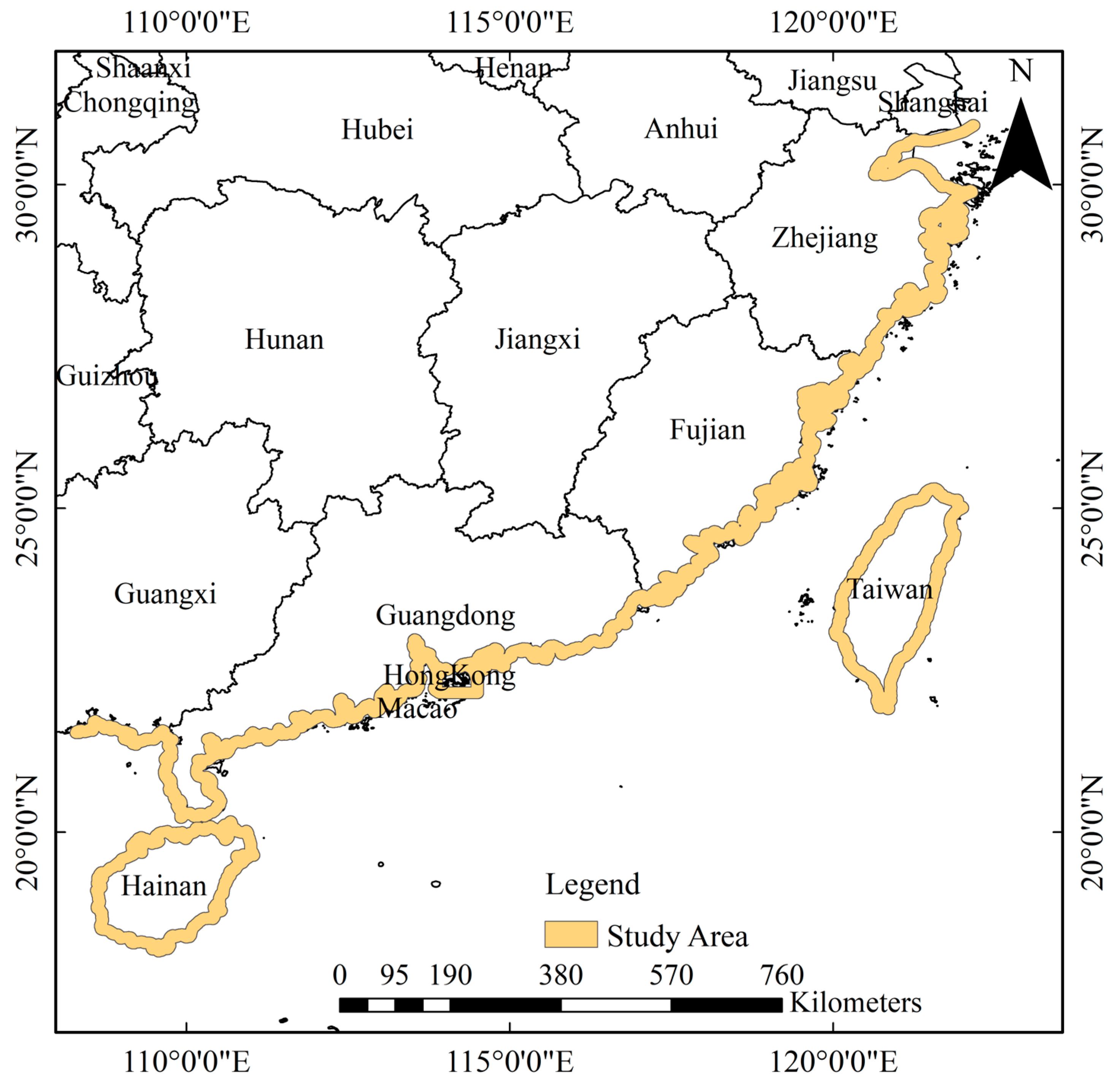
2.1. Study Area

In this study, the mangrove growth areas in China are taken as the study area, mainly including Guangxi, Guangdong, Hainan, Fujian, Zhejiang, Taiwan, Hong Kong, Macau, and other regions, located between 18°12′–31°37′ N and 108°0′–122°45′ E. The specific location is shown in Figure 1. As of 2017, there are 38 species of mangrove plants belonging to 26 genera in 22 families in China [23], mainly including Avicennia marina (Avicennia marina), Aegiceras corniculatum (Aegiceras corniculatum (L.) Blanco), Bruguiera gymnorrhiza (Bruguiera gymnorrhiza), etc. Most mangroves grow on mudflats near the coastline, with low-lying and complex terrain, often mixed with farmland, non-mangrove plants, etc.

2.2. Data Introduction and Preprocessing

2.2.1. Satellite Image Data

To accurately obtain the spatial distribution of mangroves in China in January 2021, this study used Landsat 8 images, MOD09GA, and MYD09GA as the basic data. Among them, there were 12 scenes of Landsat 8 images available in January 2021, as shown in Table 1. A total of 14 scenes of non-January 2021 Landsat 8 images were paired with MODIS data to participate in the reconstruction of the January 2021 image using the FSDAF model, as shown in Table 2. The total number of MODIS data used in January 2021 was 26, of which 15 scenes were paired with non-January 2021 Landsat 8 images, and 11 scenes participated in the reconstruction of non-January 2021 Landsat 8 images, as shown in Table 2.
The Landsat 8 image used in this study is a level 1 product from the USGS official website, so it needed to be radiometrically corrected and FLAASH atmospheric corrected using ENVI 5.3 software (Exelis Visual Information Solutions, Boulder, CO, USA) and subjected to principal component analysis (PCA). The MODIS image was obtained from the NASA official website and needed to be projected and resampled to 480 m using MRT (http://en.mrtlab.com) software (National Aeronautics and Space Administration (NASA), Washington, DC, USA). Then, in ENVI 5.3 software, the Landsat 8 image was used as a reference for geometric correction using a quadratic polynomial method, with a root mean square error (RMSE) of no more than 0.5 pixels. Finally, the nearest-neighbor method was used to resample it to 30 m.

2.2.2. Sample Data

Based on GF-1, GF-2, and Google Earth images from January 2021 and the surrounding dates, the sample points were selected with relatively obvious features throughout the study area (for the images that are not from January 2021, the sample points were selected from the same area of the image before and after January 2021 to ensure the correctness of the sample points). A total of 36,833 sample points were selected, including 10,335 mangrove samples, 5643 non-mangrove vegetation samples (including forests, crops, etc.), 9827 water samples (including oceans, lakes, ponds, etc.), and 11,028 land samples (including buildings, roads, etc.). The sample points are evenly distributed throughout the study area, as shown in Figure 2.

2.2.3. Other Auxiliary Data

To obtain a more accurate spatial distribution of mangroves, auxiliary data such as DEM were introduced and could be obtained from the ASTER GDEMV3 data from the geographic spatial data cloud, with a spatial resolution of 30 m. The elevation, slope, and slope direction were processed using ArcGIS 10.6 (Esri, Redlands, CA, USA).

2.3. Research Method

2.3.1. FSDAF Model

The FSDAF model is a spatiotemporal data fusion model proposed by Zhu et al. [20]. It predicts high-spatial-resolution images in the T2 period based on a basic image pair in the T1 period, which consists of a high-spatial-resolution image and a low-spatial-resolution image, as well as a low-spatial-resolution image in the T2 period. The basic image pair in the T1 period are close in date, and we usually selected high-quality images with little or no cloud cover. T2 usually refers to images required for research on the date.
The FSDAF model first classifies high-spatial-resolution images in the T1 period and then calculates the changes in each feature category in the low-spatial-resolution images from T1 to T2. Based on these changes, the high-spatial-resolution images in the T2 period are calculated. The resulting images achieve high accuracy for small changes in ground features but cannot accurately predict large changes in ground features. Therefore, it is necessary to introduce the residual R value to describe the ground-feature changes in low-spatial-resolution images. The FSDAF model uses a TPS function for spatial interpolation, which downscales the low-spatial-resolution images in the T2 period to more accurately allocate residuals. After the calculation is completed, the prediction of high-spatial-resolution images in the T2 period can be completed based on the changes between the high-spatial-resolution images in the T1 period and the low-spatial-resolution images from T1 to T2. Considering that the prediction process is performed pixel by pixel and that there will be patch effects during residual allocation [24], the final prediction of the high-spatial-resolution images in the T2 period is assisted by combining neighborhood information. The specific prediction process is shown in Formula (1):
T 2 ( x i j ,   y i j ) = T 1 ( x i j , y i j ) + k 1 n w k × Δ T ( x k , y k )
where T 2 ( x i j , y i j ) represents the pixel i corresponding to the predicted high-resolution image at T2, T 1 ( x i j , y i j ) represents the pixel i corresponding to the high-resolution image at T1, w k represents the weight of the kth pixel, Δ T ( x k , y k ) represents the change in the kth pixel during the T1T2 time period. The calculation process of w k and Δ T is shown in Equations (2)–(4):
w k = ( 1 / D k ) / k = 1 n ( 1 / D k )
D k = 1 + ( x k x i j ) 2 + ( y k y i j ) 2 / ( z / 2 )
Δ T ( x i j , y i j ) = R ( x i j , y i j ) + Δ T ( c )
where D k represents the spatial distance of the kth pixel, and the weight of the kth pixel is determined based on D k . z represents the size of the neighborhood. R ( x i j , y i j ) represents the residual of pixel i corresponding to low-spatial-resolution images and high-spatial-resolution images. Δ T ( c ) represents the change in the corresponding category of the pixel in the time period T1T2. The residual R value is used to approximate the change in the pixel in the time period T1T2, improving the change result of ground features. The calculation process is shown in Formula (5):
R ( x i , y i ) = 1 n j = 1 n T 1 ( x i j ,   y i j ) 1 n j = 1 n T 2 p r e ( x i j , y i j )
where n represents the number of categories, T 1 ( x i j , y i j ) represents the high-spatial-resolution image in the T1 period, and T 2 p r e ( x i j , y i j ) represents the image predicted based on the image in the T1 period. In order to better allocate the residuals, the FSDAF model introduces TPS interpolation for downscaling, which can better maintain the changes in ground feature types and local changes during the prediction process. The specific process is shown in Formula (6):
T 2 p r e ( x i j ,   y i j ) = f T P S ( x i j ,   y i j ) = a 0 + a 1 x + a 2 y + 1 2 i = 1 N b i r i 2 log r i 2
where f T P S ( x i j ,   y i j ) is the TPS interpolation method, a 0 , a 1 , a 2 are parameters determined based on the value of b i r i 2 log r i 2 , N is the pixel of the low-spatial-resolution image, and r i 2 = ( x x i ) 2 + ( y y i ) 2 .
By giving the limited-condition Formula (7), the parameters can be calculated through Formula (8). When Formula (8) reaches the minimum value, the parameters are the optimal solution:
i = 1 N b i = i = 1 N b i x i = i = 1 N b i y i = 0
1 m j = 1 m T 2 ( x i j ,   y i j ) + ξ f T P S ( x i j ,   y i j )
where m represents the number of sub-pixels in low-spatial-resolution images and ξ indicates the system difference between two different sensors.
The FSDAF model was constructed based on IDL 8.5. In order to further improve the accuracy of the model, a random forest classification algorithm with better classification capabilities was used to replace the ISODATA classification algorithm in the original model.

2.3.2. Feature Extraction

The distribution of ground objects in the investigated mangrove growth areas is relatively complex, often exhibiting the phenomena of identical objects with different spectra and different objects with identical spectra with regard to surrounding non-mangrove vegetation and farmland, leading to certain difficulties in extracting information from mangroves [25]. To accurately obtain the spatial distribution of mangroves, it is necessary to jointly apply multiple feature parameters, mainly including spectral features, exponential features, texture features, and terrain features. The specific feature parameters contained in each feature category are shown in Table 3.

2.3.3. Construction and Accuracy Evaluation of Mangrove Classification Model

Based on the extraction of feature parameters, the random forest algorithm is used to construct a model for extracting the spatial distribution of mangroves. Essentially, it consists of multiple trees that are independent of each other. Each tree samples from the sample with replacement, forming multiple decision trees [31]. Each node of each decision tree randomly selects some features during classification and obtains the optimal feature combination based on the Gini index. At the same time, each tree independently votes for the samples, and the class of the sample is determined based on the number of votes. In this way, random forests often have high accuracy in classification. During the model construction process, the parameter ntree is set to 500, and mtry is the square root of the sum of feature parameters.
The sample data were divided into modeling data and validation data in a 7:3 ratio, and 7 of the data were used for model construction. In the model construction, J–M distance and spectral differences were used to quantitatively describe the degree of sample separation. The remaining 3 data were used for model validation, and the evaluation metrics mainly included overall accuracy, user accuracy, producer accuracy, and the kappa coefficient. The specific calculation formulas are shown in reference [32].

2.3.4. Calculation of Landscape Pattern Index

Landscape pattern indexes can highly condense some information in landscape patterns and can evaluate relevant landscape types from a quantitative perspective. The classification results of mangroves based on the random forest algorithm were imported into Fragstats 4.2 software (Department of Forest Science, Oregon State University, Corvallis, OR, USA) to calculate various landscape indexes. In this study, six landscape indexes on type scale were selected, mainly including class area (CA), number of patches (NP), patch density (PD), edge density (ED), patch aggregation index (AI), and landscape shape index (LSI). The specific calculation process of each landscape index is shown in reference [33].

3. Results and Analysis

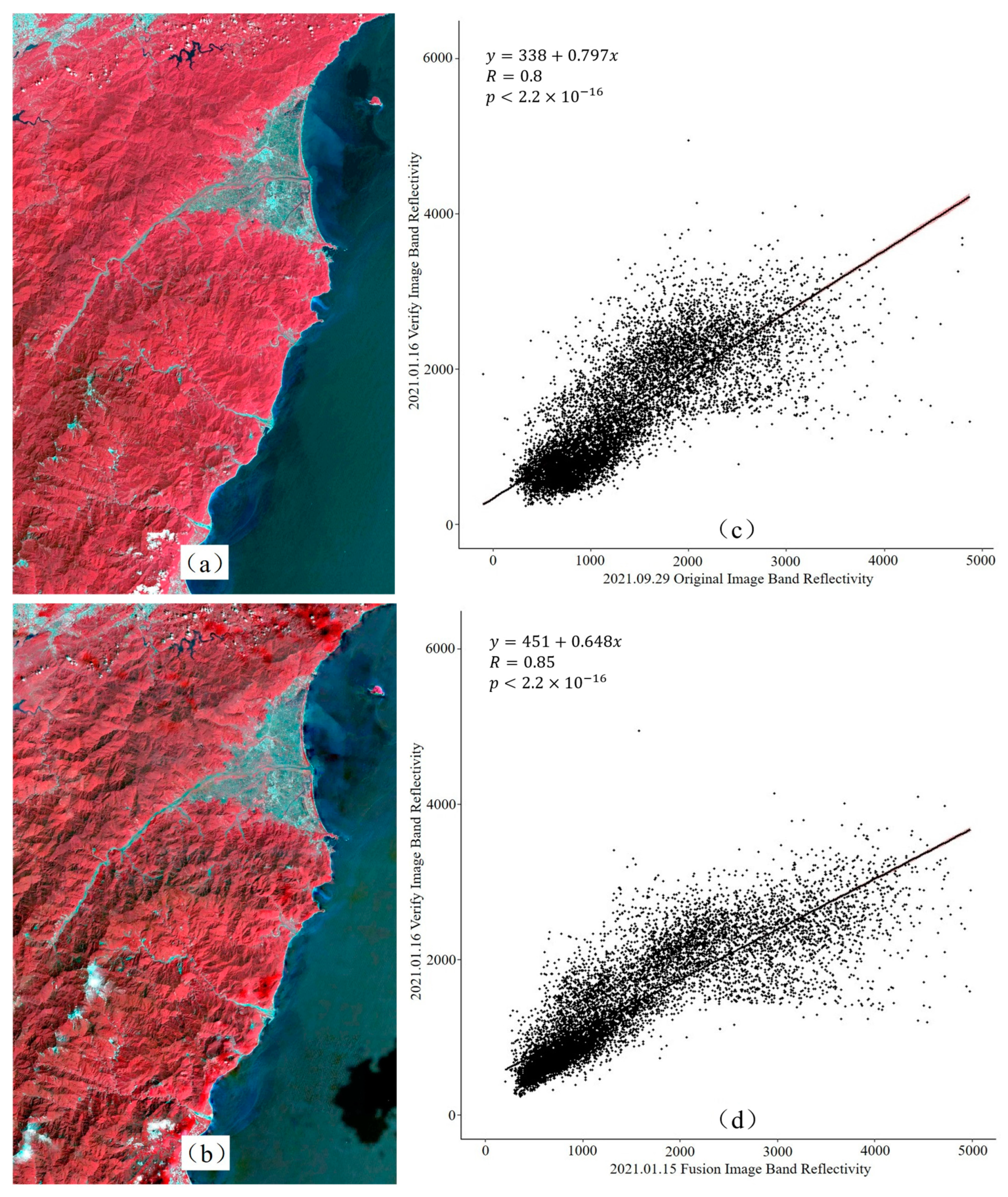
3.1. Fusion Image Based on FSDAF Model

Based on the original Landsat 8 image on 29 September 2021, a fused image on 15 January 2021 was obtained using the FSDAF model. Taking the Landsat 8 image on 16 January 2021 as the verification image, Pearson correlation analysis was used to analyze the correlation between the original image and the verification image as well as that between the fused image and the verification image. The results are shown in Figure 3.
From the results shown in Figure 3, the significance coefficients (P) of the original image and the fused image with the validation image are both less than 0.001, and the correlation coefficients ® are both greater than 0.80, indicating that there is a significant correlation between the original image and the fused image with the validation image, but the correlation between the original image and the validation image is less than that between the fused image and the validation image, as shown in Figure 3c,d. The results show that compared to the original image, the fused image obtained based on the FSDAF model is closer to the validation image and can more clearly reflect the changes in the mangroves, thus obtaining more realistic spatial distribution information of mangroves [34]. In summary, the fused image obtained based on the FSDAF model has a strong correlation with the validation image and can be used for reconstruction of images at specific times.

3.2. Mangrove Extraction Results Based on the Original Image and Fused Image

Based on the original image and the fused image with a row and column number of 125/45, the random forest algorithm was used to extract the spatial distribution of mangroves. The results are shown in Figure 4, and the classification accuracy is shown in Table 4.
As shown in Figure 4 and Table 4, the extraction results of mangroves based on the original image and the fused image are consistent in most areas, but there are slight differences in some areas, as shown in the enlarged area of Figure 4. Overall, the extraction results of mangroves based on the original Landsat 8 image on 7 October 2021 are generally lower than those based on the fused image on 2 January 2021, with the overall accuracy of the original image being 87.29%, slightly lower than the overall accuracy of the fused image of 89.97%. The user accuracy of the two images is basically the same, but there is a significant difference in producer accuracy, that is, there are more misclassifications in the original image compared to the fused image.
The reasons for the differences in the classification results of mangroves between the original image and the fused image were analyzed from the perspectives of the J–M distance and spectral curve between the mangroves and other samples. The results are shown in Table 5 and Figure 5.
According to the results shown in Table 5, for both the original image and the fused image, the J–M distance between the mangrove sample and the water sample and the land sample is higher than 1.9, indicating that the separation of the three ground objects is good, and the classification is not easily confused. For the original image of October 2021, the J–M distance between the mangrove sample and the non-mangrove vegetation sample is 1.563, which is significantly lower than the 1.768 of the January fused image, indicating that the mangrove sample and the non-mangrove vegetation sample are more difficult to distinguish regarding the original image of October than the fused image of January, resulting in a relatively poor classification result of mangroves based on the original image. By analyzing the results shown in Figure 5, the spectral curve changes specific to the fused image and the original image are similar in the blue, green, red, SWIR1, SWIR2 bands to the spectral curve changes specific to the reference image, but there are significant differences in the NIR band between the original image and the reference image. For the fused image, the difference in spectral reflectance between the mangrove and non-mangrove vegetation in the NIR band is 308.1, while the difference in spectral reflectance between the mangrove and non-mangrove vegetation in the NIR band in the reference image is 312.83, indicating that the difference between the features of the reference image and the fused image using the FSDAF model is closer in the NIR band. For the original image, the difference in spectral reflectance between the mangrove and non-mangrove vegetation in the NIR band is −19.23, indicating that the characteristics of the mangrove and non-mangrove vegetation are very similar in the NIR band of the October image, and similar spectral characteristics may lead to a smaller contribution of the NIR band reflectance and some features calculated based on the NIR band to the classification result, resulting in a poor classification result of the original image. This is also consistent with the conclusion of Li et al. [35]: that using the January image to extract mangroves can obtain more accurate results than when using the October image.

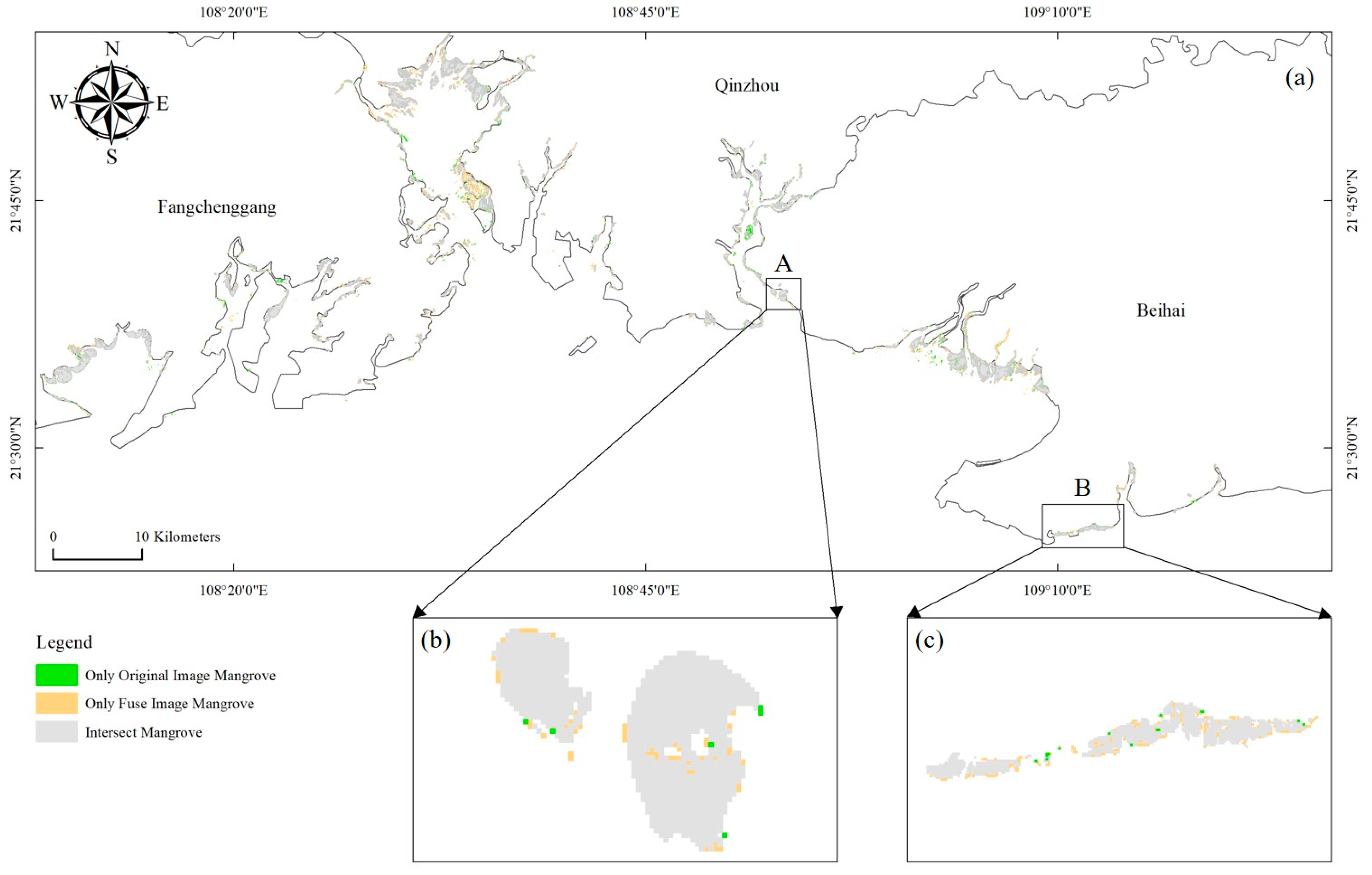
3.3. Analysis of Differences in Mangrove Extraction Results

When extracting mangroves in a large area, there is often a large time span between images due to missing data. During this period, mangroves are constantly affected by both natural and human factors, such as natural growth, disasters, human deforestation, invasive alien species, and artificial restoration [36,37], resulting in some differences between the extracted information on mangroves and the actual situation. For example, the changes in the mangroves in the two regions in different months are shown in Figure 6. After about 11 months, some mangroves in the region where mangroves originally existed disappeared, thus exposing the mudflat, as shown in the rectangular area in Figure 6a,b. In Figure 6c,d, after about 5 months, the area without mangroves grew mangroves, as shown in the rectangular area. The changes in the above images indicate that when there is a certain time span between images, the spatial distribution of mangroves undergoes certain changes. Therefore, when extracting mangroves or monitoring dynamic changes in mangroves, ignoring the time difference between images may lead to certain differences between the obtained results and the actual situation.
In order to more accurately evaluate the differences between the original image and the fused image based on the FSDAF model, the Landsat 8 image with a row and column number of 121/44 on 12 January 2021 was selected as the original image, and the Landsat 8 image on 6 December 2021 was used as the reference image. Based on the reference image, the fused image on 13 January 2021 was obtained using the FSDAF model. The tidal levels of the original image and the reference image were basically consistent, with the tidal height of the original image being 98 cm and that of the reference image being 106 cm, which allows one to basically ignore the impact of tidal inundation on the extraction of the spatial distribution of mangroves. Based on the random forest algorithm, the spatial distribution of mangroves in the original image, reference image, and fused image were extracted, and the results are shown in Figure 7.
According to the results shown in Figure 7c,d, although the spatial distributions of mangroves obtained from the original image, reference image, and fused image have little differences, the spatial distribution of mangroves extracted from the fused image is closer to that of the original image, indicating that the fused image based on the FSDAF model can simulate the changes in mangroves in images capturing different times, thus obtaining an extraction result closer to the original image [34]. However, the FSDAF model cannot fully simulate this change, which is mainly due to errors in residual allocation, that is, there are residual differences between the fused image pixels and the original image pixels. By statistically analyzing the mangrove areas extracted from the original image, reference image, and fused image, it is found that the area extracted from the original image is 239.31 ha, the area extracted from the reference image is 224.74 ha, and the area extracted from the fused image is 232.47 ha. The area of mangroves extracted from the fused image is closer to the result of the original image. Therefore, compared to previous large-scale mangrove extraction based on images from different months, the results of mangroves extracted from the same-month image based on the FSDAF model are closer to the real spatial distribution of mangroves.

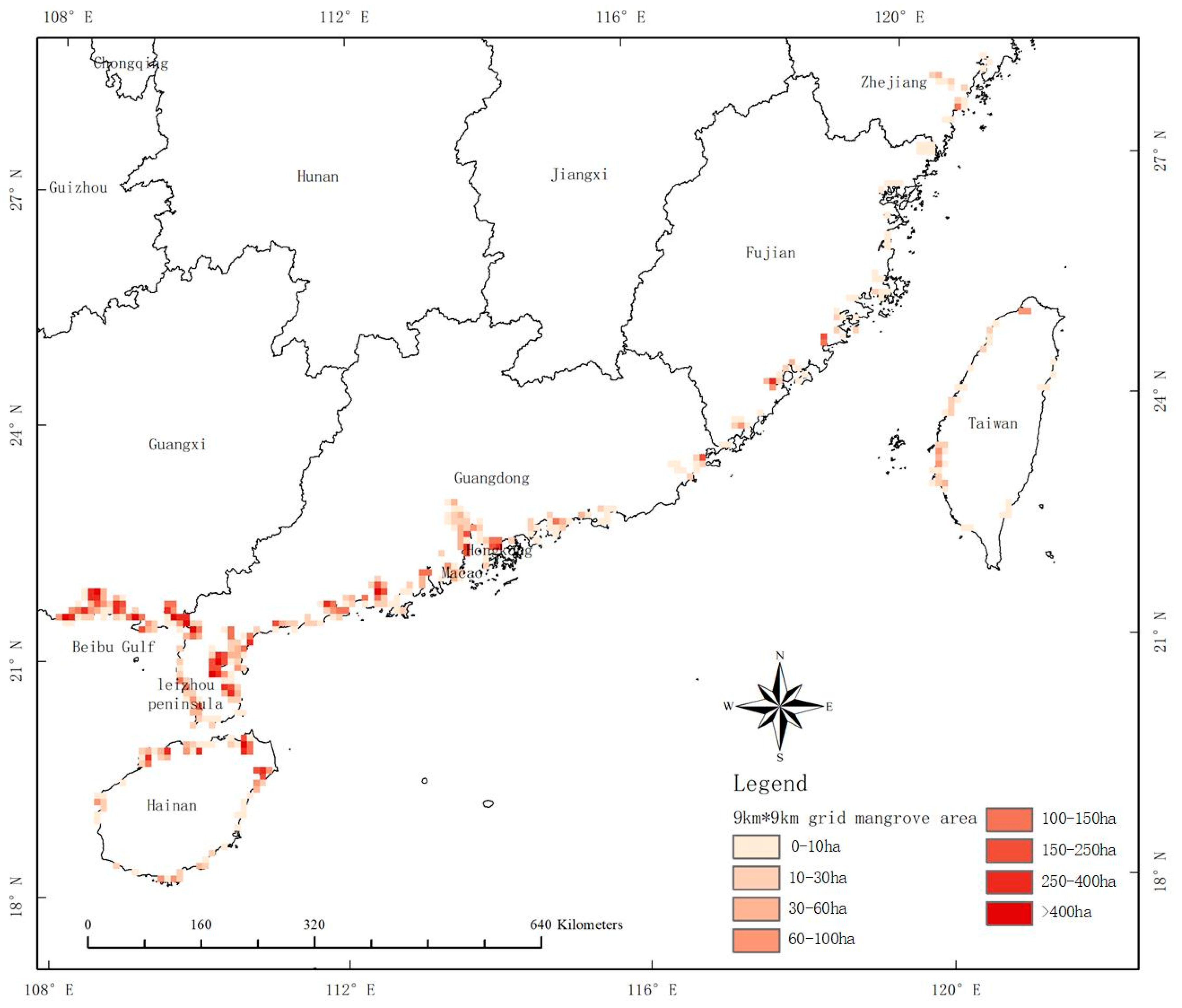
3.4. Spatial Distribution and Area Extraction Results of Mangroves in China

The spatial distribution of mangroves in China extracted from the January 2021 images reconstructed based on the FSDAF model is shown in Figure 8.
According to the analysis shown in Figure 8, China’s mangrove forests are mainly distributed in Guangxi, Guangdong, and Hainan, with relatively few forests in Zhejiang. The results show that as the latitude increases and the temperature gradually decreases, the distribution of mangroves becomes increasingly rare.
The distribution area of mangroves in relevant provinces and special administrative regions in China was statistically analyzed and represented in a 9 km × 9 km grid, as shown in Figure 9.
According to the results shown in Figure 9, the number of grids with an area of 0–10 ha is the largest, with a total of 144 grids, while the number of grids with an area of more than 400 ha is the smallest, with only 10 grids. The results show that most of China’s mangroves are distributed in the area between 108°0′ E and 114°04′ E and between 19°24′ N and 23°05′ N, with the most concentrated distribution in the Beibu Gulf and Leizhou Peninsula regions. The grids with an area of more than 400 ha are all located in this area. As the latitude increases, the distribution of mangroves becomes increasingly sparse. The grid areas of mangroves in Fujian, Zhejiang, and Taiwan are all below 60 ha, and most of the grids are below 30 ha.
The distribution area of mangroves in relevant provinces and special administrative regions in China is summarized in Figure 10.
The results shown in Figure 10 indicate that the total area of mangroves in China in January 2021 was 27,122.4 ha, of which Guangdong had the largest area of mangroves, with 12,098.34 ha, accounting for 44.61% of the total area of mangroves in the country. Guangxi, Hainan, Fujian, Hong Kong, Taiwan, Zhejiang, and Macao followed, with Macao having the smallest area of mangroves, with only 16.74 ha, accounting for 0.06% of the total area of mangroves in the country.
The mangrove area in China in January 2021 as extracted in this study is 27,122.4 ha, which is larger than similar results of previous studies. For example, Guo et al. [15] used Landsat series images to monitor the dynamic changes in mangroves in the Maritime Silk Road region from 1990 to 2015, and the mangrove area in China in 2015 was 19,144 ha. Zhang et al. [14] produced a spatial distribution map of mangroves in China with a resolution of 2 m in 2018 based on GF-1 and ZY-3 images and concluded that the area of mangroves in China in 2018 was 25,683.88 ha. This is mainly because there is a time difference between this study and previous studies, during which the area of mangroves may undergo significant changes due to the influence of natural and human factors. According to the continuous strengthening of mangrove protection and restoration in China in recent years, the area of mangroves has shown a gradual upward trend. Therefore, the mangrove area extracted in this study in 2021 should theoretically be larger than the mangrove areas extracted in 2015 and 2018 as part of previous studies. Due to the lack of relevant studies on the extraction of mangrove areas in the same year, it is not possible to conduct specific quantitative research with the mangrove areas extracted by other researchers. In the future, the spatial distribution of mangroves in different months in the same year can be extracted simultaneously to further quantify the differences in spatial distribution results of mangroves within a year. The average value of the extraction results in different months can also be taken as the accurate area of mangroves in the year to minimize the impact of accidental factors on the extraction results of the spatial distribution of mangroves.

3.5. Analysis Results of Mangrove Landscape Pattern in China

The calculation results of landscape pattern indexes of mangroves on the type scale in relevant provinces and special administrative regions in China are shown in Table 6.
According to the results shown in Table 6, from the perspective of class area, most of the mangroves are concentrated in Guangdong, Guangxi, and Hainan, with the three provinces accounting for 90.29% of the total area, reaching 24,487.47 ha. The number of patches, patch density, and edge density are often related to landscape fragmentation and human disturbance intensity. The patch density and edge density of mangroves in Fujian are the highest, with values of 2.09 and 12.59, respectively. The patch density of mangroves in Guangxi, Guangdong, Macao, and Hong Kong are all higher than 1, and the edge density is higher than 11, indicating that the patch fragmentation degree of the above regions is high and subject to significant human disturbance, resulting in low landscape security. Some mangrove growth environments may be severely damaged, requiring further strengthening of mangrove management and protection. The agglomeration index generally reflects the degree of aggregation or dispersion of landscape types. Combined with the spatial distribution of mangroves, it can be seen that suitable areas for mangroves in Hong Kong, Hainan, Guangxi, and Zhejiang are more concentrated, and the distribution of mangroves is relatively compact, resulting in a high degree of agglomeration. The areas of Guangdong, Fujian, and Taiwan span a large latitude and longitude, and the distribution of mangroves is more dispersed, resulting in a relatively low degree of aggregation index. However, the area of Macao is a special case, due to the small area of mangroves and severe human and natural impacts, resulting in a low degree of aggregation index [23]. The landscape shape index describes the regularity of the landscape shape. The larger the landscape shape index, the more irregular the shape of the landscape. The landscape shape index of mangroves is greatly affected by human and natural factors, such as artificial planting and restoration, which usually reduce the landscape shape index, while human deforestation and invasive alien species often increase the landscape shape index. The landscape shape index of mangroves in Guangdong is as high as 82.66, and the shape is extremely irregular. Guangxi, Hainan, Fujian, and Taiwan follow, with the landscape shape index of each region above 20, showing irregular shape. For these regions, it is necessary to formulate scientific mangrove restoration policies and strictly control the phenomenon of deforestation. The shape of mangroves in Hong Kong, Zhejiang, and Macao is relatively regular, benefiting from local active efforts to carry out artificial planting and restoration.

4. Conclusions

In this study, the FSDAF model was used to reconstruct the January 2021 images of the study area based on Landsat 8 and MODIS images, a random forest algorithm was used to extract the spatial distribution of mangroves, and landscape pattern indexes were analyzed. The main conclusions obtained are as follows:
(1)
The fused image based on the FSDAF model is highly similar to the reference image, with a correlation coefficient ® of 0.85. The results indicate that the fused image based on the FSDAF model has a strong correlation with the reference image and can be used for the reconstruction of images depicting specific times;
(2)
The overall accuracy of extracting the spatial distribution of mangroves from the January 2021 image reconstructed based on the FSDAF model is 89.97%, which is better than the extraction result based on the original October image (the overall accuracy is 87.29%). In January 2021, the total area of mangroves in China was 27,122.4 ha, of which Guangdong had the largest area of 12,098.34 ha, while Macao had the smallest area of 16.74 ha. Guangdong, Guangxi, and Hainan provinces accounted for 90.29% of the total area of mangroves in China;
(3)
The mangroves in Guangdong, Guangxi, Fujian, Hong Kong, and Macao are highly fragmented and severely affected by human disturbance. The mangroves in Guangxi, Hainan, Zhejiang, and Hong Kong are densely distributed and have a higher degree of aggregation. The mangroves in Guangdong and Guangxi are irregular in shape and severely affected by human logging and invasive alien vegetation. The mangroves in Zhejiang, Hong Kong, and Macao are regular in shape, thanks to active local efforts to carry out artificial restoration.
This study used the FSDAF model to reconstruct images to extract the spatial distribution of mangroves nationwide in January 2021. The results showed that the FSDAF model can accurately extract the spatial distribution of mangroves in a large area in the same month, which can improve the problem of time differences in the spatial distribution of mangroves extracted using images captured at different times. However, this study only extracted the spatial distribution of mangroves in January. In the future, the monthly spatial distribution of mangroves can be extracted to achieve more precise monitoring of dynamic changes in mangroves on a time scale. At the same time, in subsequent research, object-oriented classification can be considered to replace the pixel-based classification, reducing the “salt and pepper phenomenon” in classification results.

Author Contributions

Conceptualization, Q.Y. and H.Y.; data curation, Q.Y., W.D. and X.T.; formal analysis, Q.Y. and H.Y.; methodology, Q.Y., W.D. and Y.L.; supervision, J.C.; validation, H.Y.; writing—original draft preparation, Q.Y. and H.Y.; writing—review and editing, J.C. and Q.Y. All authors have read and agreed to the published version of the manuscript.

Funding

This study was supported by grants from the National Natural Science Foundation of China (41901370, 42261063), the Guangxi Natural Science Foundation (2018GXNSFBA281075), the Guangxi Science and Technology Base and Talent Project (GuikeAD19110064), and Scientific Research Foundation of Guilin University of Technology (GLUTQD2017094).

Data Availability Statement

No new data were created or analyzed in this study. Data sharing is not applicable to this article.

Acknowledgments

We thank the Guangxi Zhuang Autonomous Region Natural Resources Remote Sensing Institute for providing GF-2 images.

Conflicts of Interest

The authors declare no conflict of interest.

References

  1. Green, E.P.; Clark, C.D.; Mumby, P.J.; Edwards, A.J.; Ellis, A.C. Remote sensing techniques for mangrove mapping. Int. J. Remote Sens. 1998, 19, 935–956. [Google Scholar] [CrossRef]
  2. Wang, W.; Dong, Z.; Fu, D.; Qi, Y.; Lin, D. Classification of Mangrove in Leizhou Bay Based on ZY-3. Hydrogr. Surv. Charting 2020, 40, 35–39. [Google Scholar] [CrossRef]
  3. Alongi, D.M. Mangrove forests: Resilience, protection from tsunamis, and responses to global climate change. Estuar. Coast. Shelf Sci. 2008, 76, 1–13. [Google Scholar] [CrossRef]
  4. Kuenzer, C.; Bluemel, A.; Gebhardt, S.; Quoc, T.V.; Dech, S. Remote Sensing of Mangrove Ecosystems: A Review. Remote Sens. 2011, 3, 878–928. [Google Scholar] [CrossRef]
  5. Mukhopadhyay, A.; Mondal, P.; Barik, J.; Chowdhury, S.; Ghosh, T.; Hazra, S. Changes in mangrove species assemblages and future prediction of the Bangladesh Sundarbans using Markov chain model and cellular automata. Environ. Sci. Process. Impacts 2015, 17, 1111–1117. [Google Scholar] [CrossRef] [PubMed]
  6. Fan, H.; Wang, W. Some Thematic Issues for Mangrove Conservation in China. J. Xiamen Univ. (Nat. Sci.) 2017, 56, 323–330. [Google Scholar] [CrossRef]
  7. Liu, C.; Luo, Z.; Yan, Y.; Lin, H.; Hu, G.; Yu, R. Occurrence Characteristics of Microplastics in Mangrove Sediments in the Jiulong River Estuary and the Association with Heavy Metals. Environ. Sci. 2022, 43, 239–246. [Google Scholar]
  8. Jia, M. Remote Sensing Analysis of China’s Mangrove Forests Dynamics during 1973 to 2013; Northeast Institute of Geography and Agroecology, Chinese Academy of Sciences: Changchun, China, 2014. [Google Scholar]
  9. Xinqiu, D.; Baowen, L.; Zhaobai, W.; Houjian, W.; Damin, B.; Weiyu, D.; Shihao, L. Resources, Conservation Status and Main Threats of Mangrove Wetlands in China. Ecol. Environ. Sci. 2016, 25, 1237–1243. [Google Scholar] [CrossRef]
  10. Jia, M.; Wang, Z.; Mao, D.; Huang, C.; Lu, C. Spatial-temporal changes of China’s mangrove forests over the past 50 years: An analysis towards the Sustainable Development Goals (SDGs). Chin. Sci. Bull. 2021, 66, 3886–3901. [Google Scholar] [CrossRef]
  11. Zhang, Y.; Zhang, Z.; Jiang, B.; Shen, X.; Li, R. Ecosystem health assessment and management strategies of urban mangrove:A case study of Guangdong-Hong Kong-Macao Greater Bay Area. China Environ. Sci. 2022, 42, 2352–2369. [Google Scholar]
  12. Liu, K.; Li, X.; Wang, S.; Qian, J.; Zhong, K. Monitoring of the changes of mangrove wetland around the Zhujiang estuary in the past two decades by remote sensing. Trop. Geogr. 2005, 25, 111–116. [Google Scholar]
  13. Hu, L.; Xu, N.; Liang, J.; Li, Z.; Chen, L.; Zhao, F. Advancing the Mapping of Mangrove Forests at National-Scale Using Sentinel-1 and Sentinel-2 Time-Series Data with Google Earth Engine: A Case Study in China. Remote Sens. 2020, 12, 3120. [Google Scholar] [CrossRef]
  14. Zhang, T.; Hu, S.; He, Y.; You, S.; Yang, X.; Gan, Y.; Liu, A. A Fine-Scale Mangrove Map of China Derived from 2-Meter Resolution Satellite Observations and Field Data. ISPRS Int. J. Geo-Inf. 2021, 10, 92. [Google Scholar] [CrossRef]
  15. Guo, Y.; Liao, J.; Shen, G. Mapping Large-Scale Mangroves along the Maritime Silk Road from 1990 to 2015 Using a Novel Deep Learning Model and Landsat Data. Remote Sens. 2021, 13, 245. [Google Scholar] [CrossRef]
  16. Lymburner, L.; Bunting, P.; Lucas, R.; Scarth, P.; Alam, I.; Phillips, C.; Ticehurst, C.; Held, A. Mapping the multi-decadal mangrove dynamics of the Australian coastline. Remote Sens. Environ. 2020, 238, 111185. [Google Scholar] [CrossRef]
  17. Zhukov, B.; Oertel, D.; Lanzl, F.; Reinhackel, G. Unmixing-based multisensor multiresolution image fusion. IEEE Trans. Geosci. Remote Sens. 1999, 37, 1212–1226. [Google Scholar] [CrossRef]
  18. Zurita-Milla, R.; Clevers, J.G.P.W.; Schaepman, M.E. Unmixing-Based Landsat TM and MERIS FR Data Fusion. IEEE Geosci. Remote Sens. Lett. 2008, 5, 453–457. [Google Scholar] [CrossRef]
  19. Gao, F.; Masek, J.; Schwaller, M.; Hall, F. On the blending of the Landsat and MODIS surface reflectance: Predicting daily Landsat surface reflectance. IEEE Trans. Geosci. Remote Sens. 2006, 44, 2207–2218. [Google Scholar] [CrossRef]
  20. Zhu, X.; Helmer, E.H.; Gao, F.; Liu, D.; Chen, J.; Lefsky, M.A. A flexible spatiotemporal method for fusing satellite images with different resolutions. Remote Sens. Environ. 2016, 172, 165–177. [Google Scholar] [CrossRef]
  21. Yi, G.; Zhang, T.; He, Y.; Ye, H.; Li, J.; Bie, X.; Liu, D. Applicability analysis of four spatial interpolation methods for air temperature. J. Chengdu Univ. Technol. (Sci. Technol. Ed.) 2020, 47, 115–128. [Google Scholar]
  22. Zhai, H.; Huang, F.; Qi, H. Generating High Resolution LAI Based on a Modified FSDAF Model. Remote Sens. 2020, 12, 150. [Google Scholar] [CrossRef]
  23. Yang, S.; Lu, W.; Zou, Z.; Li, S. Mangrove Wetlands: Distribution, Species Composition and Protection in China. Subtrop. Plant Sci. 2017, 46, 301–310. [Google Scholar] [CrossRef]
  24. Zhu, X.; Chen, J.; Gao, F.; Chen, X.; Masek, J.G. An enhanced spatial and temporal adaptive reflectance fusion model for complex heterogeneous regions. Remote Sens. Environ. 2010, 114, 2610–2623. [Google Scholar] [CrossRef]
  25. Hu, L.; Li, W.; Xu, B. Monitoring mangrove forest change in China from 1990 to 2015 using Landsat-derived spectral-temporal variability metrics. Int. J. Appl. Earth Obs. Geoinf. 2018, 73, 88–98. [Google Scholar] [CrossRef]
  26. Huete, A.; Didan, K.; Miura, T.; Rodriguez, E.P.; Gao, X.Y.; Ferreira, L.G. Overview of the radiometric and biophysical performance of the MODIS vegetation indices. Remote Sens. Environ. 2002, 83, 195–213. [Google Scholar] [CrossRef]
  27. Xu, H. A Study on Information Extraction of Water Body with the Modified Normalized Difference Water Index (MNDWI). Natl. Remote Sens. Bull. 2005, 9, 589–595. [Google Scholar] [CrossRef]
  28. Gitelson, A.A.; Kaufman, Y.J.; Stark, R.; Rundquist, D. Novel algorithms for remote estimation of vegetation fraction. Remote Sens. Environ. 2002, 80, 76–87. [Google Scholar] [CrossRef]
  29. Pintym, B.; Verstraete, M.M. GEMI: A non-linear index to monitor global vegetation from satellites. Vegetatio 1992, 101, 15–20. [Google Scholar] [CrossRef]
  30. Zha, Y.; Ni, S.; Yang, S. An Effective Approach to Automatically Extract Urban Land-use from TM Imagery. Natl. Remote Sens. Bull. 2003, 7, 37–40. [Google Scholar] [CrossRef]
  31. Breiman, L. Random Forests. Mach. Learn. 2001, 45, 5–32. [Google Scholar] [CrossRef]
  32. Ye, Z.; Guo, Q.; Zhang, J.; Zhang, H.; Deng, H. Extraction of urban impervious surface based on the visible images of UAV and OBIA-RF algorithm. Trans. Chin. Soc. Agric. Eng. 2022, 38, 225–234. [Google Scholar] [CrossRef]
  33. Wu, J. Landscape Ecology: Pattern, Processe, Scale and Hierarchy, 2nd ed.; Higher Education Press: Beijing, China, 2007. [Google Scholar]
  34. Deng, W.; You, H.; Lei, P.; Li, M.; Chen, J. Monitoring of monthly dynamic changes of mangroves based on the FSDAF model. J. Cent. South Univ. For. Technol. 2022, 42, 27–39. [Google Scholar] [CrossRef]
  35. Li, H.; Jia, M.; Zhang, R.; Ren, Y.; Wen, X. Incorporating the Plant Phenological Trajectory into Mangrove Species Mapping with Dense Time Series Sentinel-2 Imagery and the Google Earth Engine Platform. Remote Sens. 2019, 11, 2479. [Google Scholar] [CrossRef]
  36. Nguyen, H.-H.; Nguyen, C.T.; Vo, N.D. Spatial-temporal dynamics of mangrove extent in Quang Ninh Province over 33 years (1987–2020): Implications toward mangrove management in Vietnam. Reg. Stud. Mar. Sci. 2022, 52, 102212. [Google Scholar] [CrossRef]
  37. Phan, M.H.; Stive, M.J.F. Managing mangroves and coastal land cover in the Mekong Delta. Ocean Coast. Manag. 2022, 219, 106013. [Google Scholar] [CrossRef]
Figure 1. Location of the study area.
Forests 14 02399 g001
Figure 2. Distribution of some sample points used in the study.
Forests 14 02399 g002
Figure 3. Image fusion results: (a) original Landsat 8 image on 25 September 2021; (b) fused image on 15 January 2021; (c) scatter plot of correlation between original image and validation image; (d) scatter plot of correlation between fused image and validation image.
Forests 14 02399 g003
Figure 4. The extraction results of mangroves’ spatial distribution: (a) the extraction results from the original Landsat 8 image on 7 October 2021 and the fused image on 2 January 2021; (b) enlarged result of area A; (c) enlarged result of area B.
Forests 14 02399 g004
Figure 5. Comparison results of the spectral curves of mangroves and other vegetation: (a) reference image on 19 January 2022; (b) fused image on 2 January 2021; (c) original image on 7 October 2021.
Forests 14 02399 g005
Figure 6. Changes in mangrove forests based on historical images from Google: (a) January 2019; (b) December 2019; (c) June 2020; (d) November 2020.
Forests 14 02399 g006
Figure 7. The extraction results of spatial distribution of mangroves based on different images: (a) Guangdong province; (b) spatial distribution of mangroves in Huizhou and Shanwei; (c) extraction results of mangroves in Huizhou; (d) extraction results of mangroves in Shanwei.
Forests 14 02399 g007
Figure 8. Spatial distribution of mangroves in relevant provinces and special administrative regions in China: (a) China; (b) Zhejiang; (c) Fujian; (d) Guangxi; (e) Hongkong; (f) Taiwan; (g) Guangdong; (h) Hainan; (i) Macao.
Forests 14 02399 g008
Figure 9. 9 km × Distribution of mangroves in China in a 9 km × 9 km grid.
Forests 14 02399 g009
Figure 10. Statistics of mangrove distribution areas in relevant provinces and special administrative regions of China: (a) bar chart; (b) pie chart.
Forests 14 02399 g010
Table 1. Landsat 8 images available in January 2021.
Landsat
Path/Row
Landsat
Date
Landsat
Path/Row
Landsat
Date
Landsat
Path/Row
Landsat
Date
Landsat
Path/Row
Landsat
Date
117/4516 January 2021119/4114 January 2021119/4214 January 2021119/4314 January 2021
120/4321 January 2021121/4412 January 2021121/4512 January 2021122/4419 January 2021
124/451 January 2021124/461 January 2021124/471 January 2021125/4724 January 2021
Table 2. Landsat 8 and MODIS images from dates outside of January 2021 and MODIS images from January 2021.
LandsatMODISPaired MODIS Data DateReconstructed Image
Path/RowDatePath/Row(MOD/MYD/Mosaic) 1Date 2Band Number 3
117/4329 September 2021H28/V06, H29/V0630 September 2021 (MOD Mosaic)15 January 20216
117/441 February 2021H29/V066 February 2021 (MOD)26 January 20216
118/3922 December 2020H28/V05, H29/V0621 December 2020 (MOD Mosaic)29 January 20216
118/4022 December 2020H28/V0631 December 2020 (MYD)13 January 20215
118/4110 April 2020H28/V069 April 2020 (MOD)15 January 20216
118/4210 April 2020H28/V069 April 2020 (MOD)15 January 20216
118/437 November 2021H28/V06, H29/V0611 November 2021 (MYD Mosaic)13 January 20215
118/447 November 2021H29/V066 November 2021 (MOD)15 January 20216
120/446 February 2021H28/V064 February 2021 (MYD)13 January 20215
122/454 February 2021H28/V064 February 2021 (MYD)31 January 20215
123/457 November 2020H28/V067 November 2020 (MYD)18 January 20215
123/4619 June 2021H28/V06, H28/V0720 June 2021 (MOD Mosaic)18 January 20216
123/4719 June 2021H28/V0720 June 2021 (MOD)18 January 20216
125/457 October 2021H28/V0626 October 2021 (MOD)2 January 20216
Note: 1 MOD refers to MOD09GA data, MYD refers to MYD09GA data, and Mosaic refers to the data after splicing the two scenes of MODIS data; 2 the date of the reconstructed image is both the date of the MODIS data involved in the prediction and the date of the fused image predicted; 3 due to the inability of MODIS band 5 to correspond to Landsat 8 image bands, the reconstructed image only has 6 bands. At the same time, due to the presence of stripes in band 6 of some MODIS images, some images have band 6 (short-wave infrared 1) removed, resulting in some images only having 5 bands (blue, green, red, near-infrared, and short-wave infrared 2) after reconstruction.
Table 3. Statistical table of extracted feature parameters.
Feature CategoryQuantitySpecific ParametersInstructions
Spectral8–10Band1-7, PCA-1, PCA-2, PCA-3The spectral features of the original Landsat image are band 1–7. The reconstructed Landsat image lacks band 1 (coastal). Some of the reconstructed Landsat images lack band 1 and band 6 (SWIR1) due to the presence of a stripe in MODIS band 6 that cannot participate in the reconstruction. In addition, all images were subjected to PCA, and the first three principal components (PCA-1, PCA-2, PCA-3) were fused with the original bands.
Texture24Mean, Var, Hom, Con, Ent, Cor, ASM, DisThe texture features of the first three principal components (PCA-1, PCA-2, PCA-3) of each image are calculated using a grayscale co-occurrence matrix.
Index7NDVI [26] N D V I = R N I R R R e d R N I R + R R e d
MNDWI [27] 1 M N D W I = R G r e e n R S W I R R G r e e n R S W I R
EVI [26] E V I = 2.5 × R N I R R R e d R N I R + 6 R R e d 7.5 R B l u e + 1
GNDVI [28] G N D V I = R N I R R G r e e n R N I R + R G r e e n
GEMI [29] G E M I = ɳ ( 1 0.25 ɳ ) ( R R e d 0.125 1 R R e d )
Among them: ɳ = 2 ( R N I R 2 R R e d 2 ) + 1.5 R N I R + 0.5 R R e d R N I R + R R e d + 0.5
NDBI [30] N D B I = R S W I R R N I R R S W I R + R N I R
Terrain3Slope direction, slope, elevationSlope direction, slope, and elevation information can be calculated using ArcGIS 10.6.
1 The SWIR band of MNDWI and NDBI usually refers to the SWIR1 band. For fused Landsat images without a SWIR1 band, the SWIR2 band is used instead.
Table 4. Evaluation results of mangrove extraction accuracy based on original images and fused images.
Original Landsat 8 Image on 7 October 2021Fusion Image on 2 January 2021
UA92.17%92.40%
PA89.36%93.08%
OA87.29%89.97%
Kappa0.800.84
Table 5. Statistical results of J–M distance between mangrove and other samples.
Mangrove_Original ImageMangrove_Fusion Image
Water1.9991.998
Land1.9961.960
Other_tree1.5631.768
Table 6. The calculation results of landscape pattern indexes of mangroves on the type scale in relevant provinces and special administrative regions in China.
CA (ha)NP (Number)PD (No./100 ha)ED (m)AI (%)LSI
Guangdong12,098.3439591.5712.8877.6482.66
Guangxi7642.1720441.7513.2283.0150.33
Hainan4746.969610.807.4483.6438.34
Fujian1085.944602.0913.5977.6125.34
Hongkong657.09671.0712.7188.1211.02
Taiwan635.672680.865.8373.9822.49
Zhejiang239.49820.352.4981.9410.06
Macao16.74101.6711.3375.294.04
Disclaimer/Publisher’s Note: The statements, opinions and data contained in all publications are solely those of the individual author(s) and contributor(s) and not of MDPI and/or the editor(s). MDPI and/or the editor(s) disclaim responsibility for any injury to people or property resulting from any ideas, methods, instructions or products referred to in the content.

