Research on Estimating and Evaluating Subtropical Forest Carbon Stocks by Combining Multi-Payload High-Resolution Satellite Data

Abstract

Forest carbon stock is an important indicator reflecting the structure of forest ecosystems and forest quality, and an important parameter for evaluating the carbon sequestration capacity and carbon balance of forests. It is of great significance to study forest carbon stock in the context of current global climate change. To explore the application ability of multi-loaded, high-resolution satellite data in the estimation of subtropical forest carbon stock, this paper takes Huangfu Mountain National Forest Park in Chuzhou City as the study area, extracts remote sensing features such as spectral features, texture features, backscattering coefficient, and other remote sensing features based on multi-loaded, high-resolution satellite data, and carries out correlation analyses with the carbon stock of different species of trees and different age groups of forests. Regression models for different tree species were established for different data sources, and the optimal modeling factors for multi-species were determined. Then, three algorithms, namely, multiple stepwise regression, random forest, and gradient-enhanced decision tree, were used to estimate carbon stocks of multi-species, and the predictive ability of different estimation models on carbon stocks was analyzed using the coefficient of determination (R²) and the root mean square error (RMSE) as indexes. The following conclusions were drawn: for the feature factors, the texture features of the GF-2 image, the new red edge index of the GF-6 image, the radar intensity coefficient sigma, and radar brightness coefficient beta of the GF-3 image have the best correlation with the carbon stock; for the algorithms, the random forest and gradient-boosting decision tree have the better effect of fitting and predicting the carbon stock of multi-tree species, among which gradient-boosting decision tree has the best effect, with an R² of 0.902 and an RMSE of 10.261 t/ha. In summary, the combination of GF-2, GF-3, and GF-6 satellite data and gradient-boosting decision tree obtains the most accurate estimation results when estimating forest carbon stocks of complex tree species; multi-load, high-resolution satellite data can be used in the inversion of subtropical forest parameters to estimate the carbon stocks of subtropical forests. The multi-loaded, high-resolution satellite data have great potential for application in the field of subtropical forest parameter inversion.

1. Introduction

The forest ecosystem is the main body and largest carbon pool of the terrestrial ecosystem and plays an indispensable role in mitigating global climate change [1,2]. Although only about 31% of the world’s total land area is forested [3,4], its vegetation carbon stock accounts for more than 86% of the global vegetation carbon stock [5]. In our country, subtropical forests account for about half of the forest area, and subtropical forest biomass is one of the regions with the largest estimates of vegetation biomass in the world and is an important component of forest carbon stocks [6]. Studies on forest carbon stocks at home and abroad mainly focus on the tropical and temperate regions, while there are relatively few studies on subtropical forests in eastern China, making it impossible to fully understand the contribution of this region to the global carbon cycle [7]. Therefore, accurate estimation of subtropical forest carbon storage and understanding its role in the global carbon cycle is the future research direction [8].

Forest carbon storage estimation using remote sensing technology currently faces the following problems: (1) the lack of remote sensing estimation of forest carbon stock considering the factors of different tree species and forest age. In a forest ecosystem, the carbon allocation process between aboveground and belowground vegetation is influenced by climatic factors, site conditions, forest types, forest management, and age structure [9,10]; in particular, tree species and age are especially important for estimating forest ecosystem carbon stocks at regional scales [11,12]. In recent years, a great deal of research has been carried out on the carbon storage and distribution characteristics of plantations with different tree species and ages at the regional scale. At present, many researchers have studied the changes of forest carbon storage and distribution patterns with forest age. The results show that forest age has a good response to the estimation of forest carbon storage. (2) Modeling the estimation of forest carbon stocks requires finding remote sensing features with high correlation with forest carbon stocks, and the process of finding quantitative relationships between forest carbon stocks and remote sensing features is difficult. As far as remote sensing data itself is concerned, passive remote sensing images are widely used for monitoring land change and forest resources, and the spectral information can effectively reflect the growth of vegetation [13,14]. Longer wavelengths of SAR such as L-band and P-band are more relevant in estimating biomass carbon stocks [15]. LiDAR can penetrate a vegetation canopy to obtain detailed vertical structure information of the stand or forest, which theoretically allows for more accurate estimation of forest parameters [16,17,18,19]. Studies such as Yue et al. have found that combining Gedi and Sentinel-2 data to estimate dense canopy heights can accurately predict forest carbon stocks [20]. As early as in the process of estimating biomass by remote sensing, researchers have found that the survey of traditional forest aboveground biomass (AGB) plots is time-consuming and laborious; however, remote sensing data are widely used in large-scale forest AGB estimation because of their high correlation between spectral information and vegetation parameters and the ability to capture large-scale land surface features continuously [21,22]. Studies based on WordView-2 images, such as Eckert et al., have found that texture features have a better correlation with biomass than spectral information [23]. It has been shown that there is a strong correlation between biomass and SAR backscattering coefficient [24]. Remote sensing studies of tropical forest biomass in Cameroon have shown a good correlation between the mid-infrared vegetation index and the total biomass of tropical forest vegetation [25]. (2) The linear regression model and machine learning model are used as the main estimation models for estimating biomass carbon stock by remote sensing at present [26]. The random forest algorithm is one of the commonly used algorithms for the idea of bagging in integrated learning, and it belongs to the machine learning models with better performance in estimating forest carbon stock [27]. Gradient-boosting decision trees are one of the common algorithms for boosting ideas in integrated learning, but they are seldom used to estimate forest carbon stock. Also missing is a comparison of the estimation capabilities of gradient-boosted decision trees (GBDT) and random forest algorithms in regression prediction problems. Gradient-boosting decision tree (GBDT) is a learning algorithm based on CART, which uses the negative gradient value of the loss function of the model as the approximate value of residuals to fit the regression tree; the additive model is used to make a linear combination of the regression trees generated by the sub-iteration to get the final classifier [28]. The gradient-promoted decision tree (GBDT) algorithm performs better than random forests in solving nonlinear problems [29], and the main advantage of this model is that it can solve multicollinearity problems by involving all explanatory variables [30]. It is very sensitive to outliers and improves performance by reducing model deviation.

In this study, we mainly want to analyze the correlation between multiple eigenvectors extracted from multi-loaded, high-resolution satellite data and forest carbon stock and obtain the eigenvectors with better responses to forest carbon stock according to species responses and age group to participate in modeling. While comparing the estimation accuracy of two different thought models, random forest and gradient decision tree, in the prediction of carbon stock in multi-tree species, we aim to provide a certain scientific basis and theoretical support for remote sensing estimation of carbon stock in subtropical forests.

2. Materials and Methods

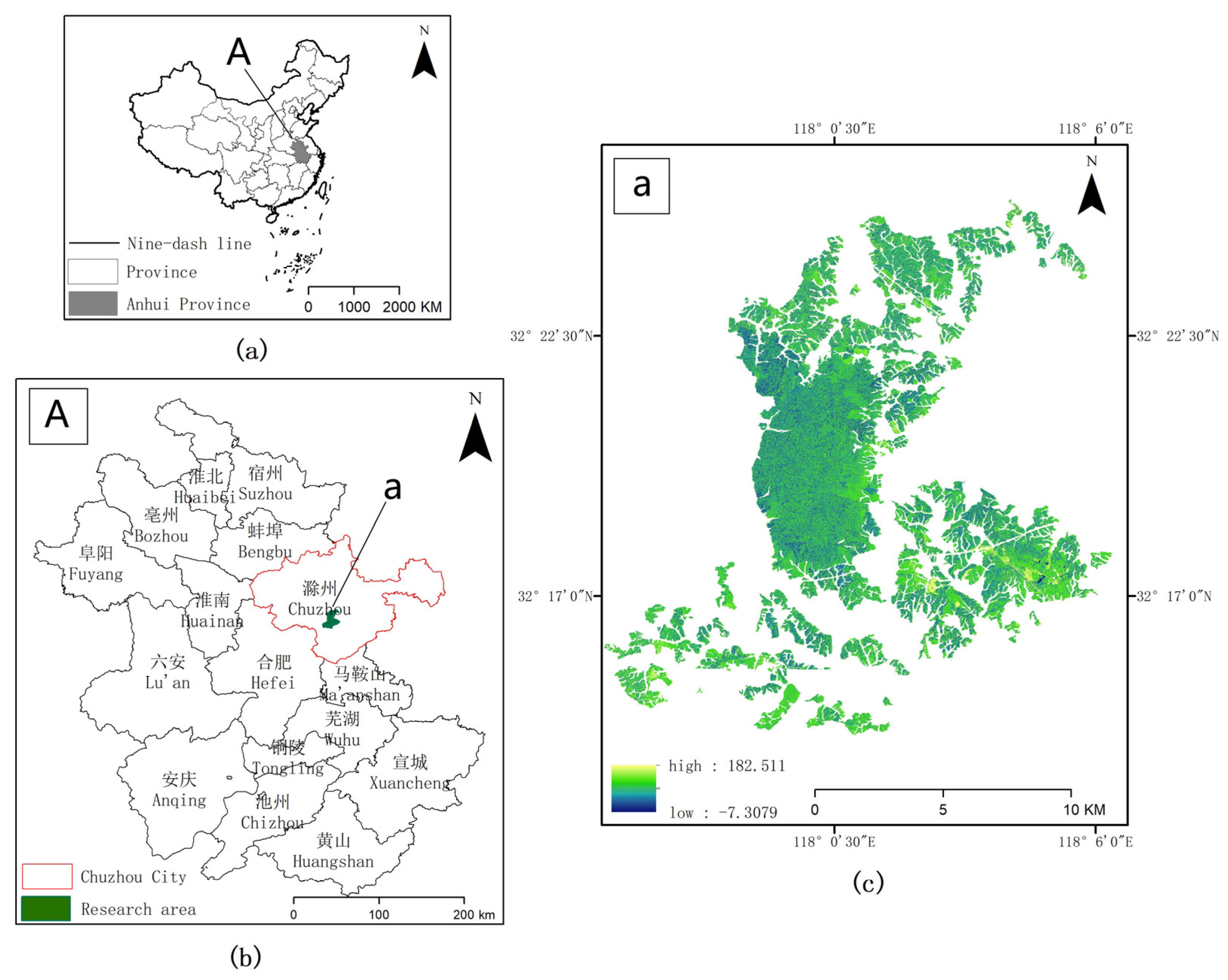
2.1. Study Area

Huangfu Mountain National Forest Park is located in the northwest of Chuzhou City, located in the hilly area of Jianghuai Province. The geographical coordinates are 117°58′ to 118°03′ in the east and 32°17′ to 32°25′ in the north. It is the largest primary secondary forest in the Jianghuai watershed of China. The forest farm is located on the northern edge of the subtropical zone, with an average annual temperature of 14.3 °C and an average annual precipitation of 1060 mm. The vegetation is a primary secondary forest with 96% forest coverage. According to the 2012 forest type II survey data, forest types include coniferous, deciduous broad-leaved, temperate broadleaf and mixed forest and mixed coniferous and broadleaved forests. Among them, Pinus massoniana, Slash pine, and Quercus acutissima account for more than 78.2% of the whole forest. So this article chooses these three tree species as the main tree species in the whole forest area on which to carry out our analysis. The following shows a schematic of the study area for this paper (Figure 1).

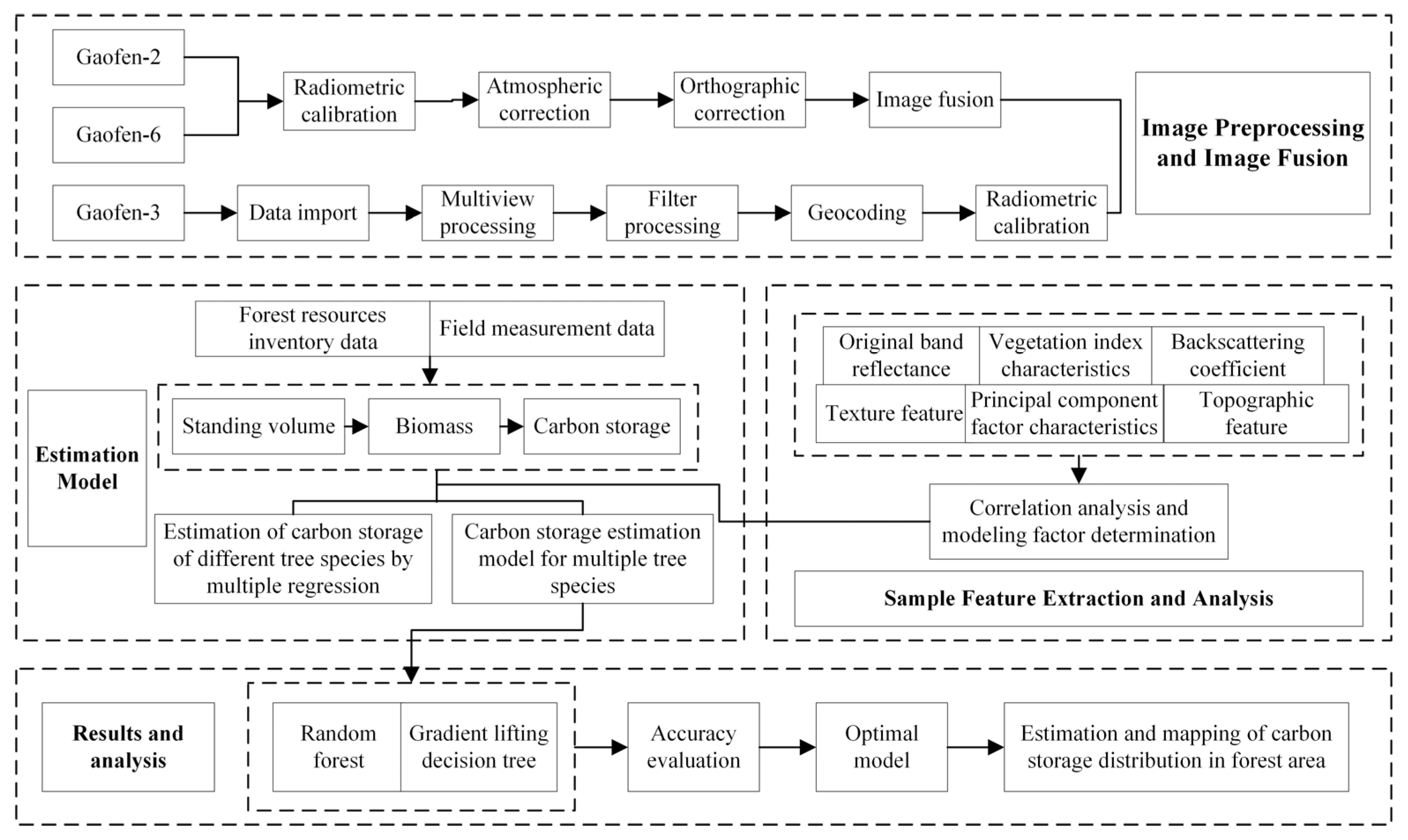
2.2. Technology Roadmap

This paper mainly starts from four aspects: data preprocessing, feature factor extraction and analysis, forest carbon storage estimation model construction, and mapping and discussion of forest carbon storage distribution based on forest carbon storage estimation results. The following is the technical roadmap of this paper (Figure 2).

2.3. Data

2.3.1. Remote Sensing Image

We choose GF-6 level of processing WFV image data on 30 July 2020, GF-2 image data on 3 September 2020, and GF-3 image data on 14 September 2020. GF-6 WFV data have a single-scene width of 800 km and a spatial resolution of 16 m. In addition to the traditional multispectral bands (B1–B4: 0.45–0.89), new bands have been added: red edge I (B5: 0.69–0.73), red edge II (0.73–0.77), purple edge (B7: 0.40–0.45), and yellow edge (B8: 0.59–0.62). GF-2 is the first civil optical remote sensing satellite with better spatial resolution than 1 m developed by China. It carries two high-resolution 1 m panchromatic and 4 m multispectral cameras. GF-3 is China’s first civilian C-band synthetic aperture radar satellite, with 12 imaging modes including scan mode, strip mode, spotlight mode, and azimuth multi-beam mode [31]. The images selected in this paper can cover the study area well.

Based on ENVI software 5.6 (Exelis Visual Information Solutions, Inc., Boulder, CO, USA), GF-2, GF-3, and GF-6 image processing, the China Resources Satellite Application Centre officially calibrated the GF-2 PMS1 sensors and GF-6 absolute radiation sensor calibration coefficient, as well as the wave spectral response function, to calibrate the radiation and perform atmospheric correction. The ortho-correction uses 30 m DEM data as the terrain correction data, and the correction points are selected based on Google offset-free images to correct geometric distortions generated by the system and to reduce geometric distortions induced by the terrain [32]. In the correction process, we use the rational polynomial geometric fine correction model, which is a general imaging sensor model for high-resolution satellite imagery, to obtain a spatial resolution of 16 m for the corrected GF-6. The corrected GF-2 4 m multispectral and 1 m panchromatic data were fused by the NNDiffuse Pan Sharpening fusion method, and the spatial resolution was 1 m.

Secondary data, including terrain data (DEM), uses the DEM data to extract elevation, gradient, and slope direction information of the research area. These terrain factors are then used in the construction of the feature set. The ground reference system used for the spatial data in this paper is the World Geodetic System-1984, and the projection is Universal Transverse Mercator.

2.3.2. Ground Survey Data

This article is based on the 2018 sample survey information from the HuangFuShan Forest Farm field. The sample data include the estimation of carbon reserves for 315 small class samples. Sample plot survey data include sample plot species composition, dominant tree species, average diameter at breast height (DBH), average tree height, degree of depression, forest age, hectare volume, slope, slope direction, elevation, and other basic information of the sample plot. Please refer to

Table 1. Basic information on forest sample plot parameters.

Plot	Number of Places	DBH/cm		Height of Tree/m		Trees/ha	Crown Density
		Range	Average	Range	Average	Range	Average	Range
Single species	283	5.21–18.36	12.02	2.41–15.12	7.36	752~2951	1674	0.6~0.9
Pinus massoniana	123	6.21~18.28	13.28	5.86~13.12	7.42	752~2745	1821	0.8~0.9
Slash pine	69	6.61–18.32	14.41	3.05~8.56	7.44	825~2350	1706	0.8~0.9
Quercus acutissima	52	6.12~15.22	9.01	2.62~9.56	5.52	725~2851	1224	0.9
Broadleaf forest	22	5.15~15.20	8.41	4.56~9.75	4.14	752~2125	1114	0.8~0.9
Coniferous forest	17	6.15~18.36	14.68	4.52~8.56	7.81	752~2359	1350	0.8~0.9
Needle and broad-leaved Mixed forest	32	6.15–16.16	10.28	3.21~8.56	4.92	1440~2550	1241	0.7~0.9

for more details.

This research primarily focuses on the main advantages of small class sizes in three tree species: Pinus massoniana, Quercus acutissima, and Slash pine. According to the forestry industry standards of the People’s Republic of China, the forest ecosystem carbon measurement guide provides the following guidelines for calculating the carbon content of aboveground parts of trees. This calculation is based on the average aboveground biomass per unit area of each tree species, the carbon content of each tree species, and the forest area. To obtain the carbon coefficient, the following method should be used:

(a)

In the ecosystem carbon pool survey, the results are used to determine the carbon content and tree species present.

(b)

According to the table of biomass conversion parameters for major dominant tree species (groups), the main advantages of tree species biomass conversion parameters are as follows.

(c)

Using the default 0.5 tC/T.D.M.

According to the “Biomass Model and Carbon Measurement Parameters” by the People’s Republic of China, carbon coefficients are determined for each part of the tree for Pinus massonianaiana, Slash pine, and Quercus acutissima. The corresponding coefficients for each species are shown in Table 1 and

Table 2. Carbon content of different tree species.

Forest Tree Species	Coefficient of Carbon
Pinus massoniana	0.5254
Slash pine	0.4756
Quercus acutissima	0.4827
Broad-leaved mixed forest	0.4900

.

2.4. Feature Extraction

Remote sensing data have been widely used in forestry resource investigation and estimation. Relevant studies [33,34,35] have shown that there is a significant correlation between forest carbon storage and remote sensing characteristic variables. The main remote sensing feature variables selected in this study are optical image features, including spectral reflectance, vegetation index, texture feature and backscattering coefficient of the radar image.

2.4.1. Optical Image Features

(1)

The Surface Reflectance

Spectral information was obtained by selecting GF-2 images and GF-6 band images. In addition to the original four bands of GF-2, eight bands from GF-6 were added, resulting in a total of twelve bands of information. The surface reflectance of the four multispectral bands of the extracted GF-2 image is shown in Figure 3.

(2)

The Characteristics of Vegetation Index

Based on the original spectral information, in order to improve the estimation of vegetation carbon, several common vegetation indexes were used. These include the normalized difference vegetation index (NDVI), the ratio vegetation index (RVI), the difference index (DVI), enhanced vegetation index (EVI), soil-adjusted vegetation index (SAVI), green degree of normalized difference vegetation index (GNDVI), and infrared percentage difference vegetation index (IPVI). Domestic GF-6 Satellite adds red edge bands closer to Sentinel-2’s 5th and 6th bands. The introduction of biomass application in Sentinel-2 data has shown high sensitivity to two planting indexes, MTCI and NDREI [36]. MTCI is particularly sensitive to chlorophyll content in plant leaves, with the ratio being proportional to chlorophyll content. NDREI, on the other hand, is used for vegetation classification and leaf area index calculation, based on the peaks and troughs of red edge normalized processing [37]. The pre-processed GF-6 image bands were operated using ENVI’s Band Math (Band Math) tool to obtain nine vegetation indices. The formula for calculating the vegetation index is shown in

Table 3. Commonly used vegetation index.

Vegetation Index	A Formula to Calculate
RVI	$RVI={\rho }_{NIR}/{\rho }_{RED}$
NDVI	$NDVI=\frac{{\rho }_{NIR}-{\rho }_{RED}}{{\rho }_{NIR}+{\rho }_{RED}}$
EVI	$EVI=2.5\times \frac{{\rho }_{NIR}-{\rho }_{RED}}{{\rho }_{NIR}+6.0\times {\rho }_{RED}-7.5\times {\rho }_{BLUE}+1}$
DVI	$DVI={\rho }_{NIR}-{\rho }_{RED}$
SAVI	$SAVI=\frac{({\rho }_{NIR}-{\rho }_{RED})}{({\rho }_{NIR}+{\rho }_{RED}+L)}\times (1+L)$
GNDVI	$GNDVI=\frac{{\rho }_{NIR}-{\rho }_{GREEN}}{{\rho }_{RED}+{\rho }_{GREEN}}$
IPVI	$IPVI={\rho }_{NIR}/({\rho }_{NIR}+{\rho }_{RED})$
MTCI	$MTCI=({\rho }_{0.75}-{\rho }_{0.71})/({\rho }_{0.71}-{\rho }_{RED})$
NDREI	$NDRE1=(B_{0.75}-B_{0.71})/(B_{0.75}+B_{0.71})$

Note: in the formula, NIR for near infrared band; L as the adjustment coefficient of soil; in this study, take 0.5.

, and the extraction of various vegetation indices is shown in Figure 4.

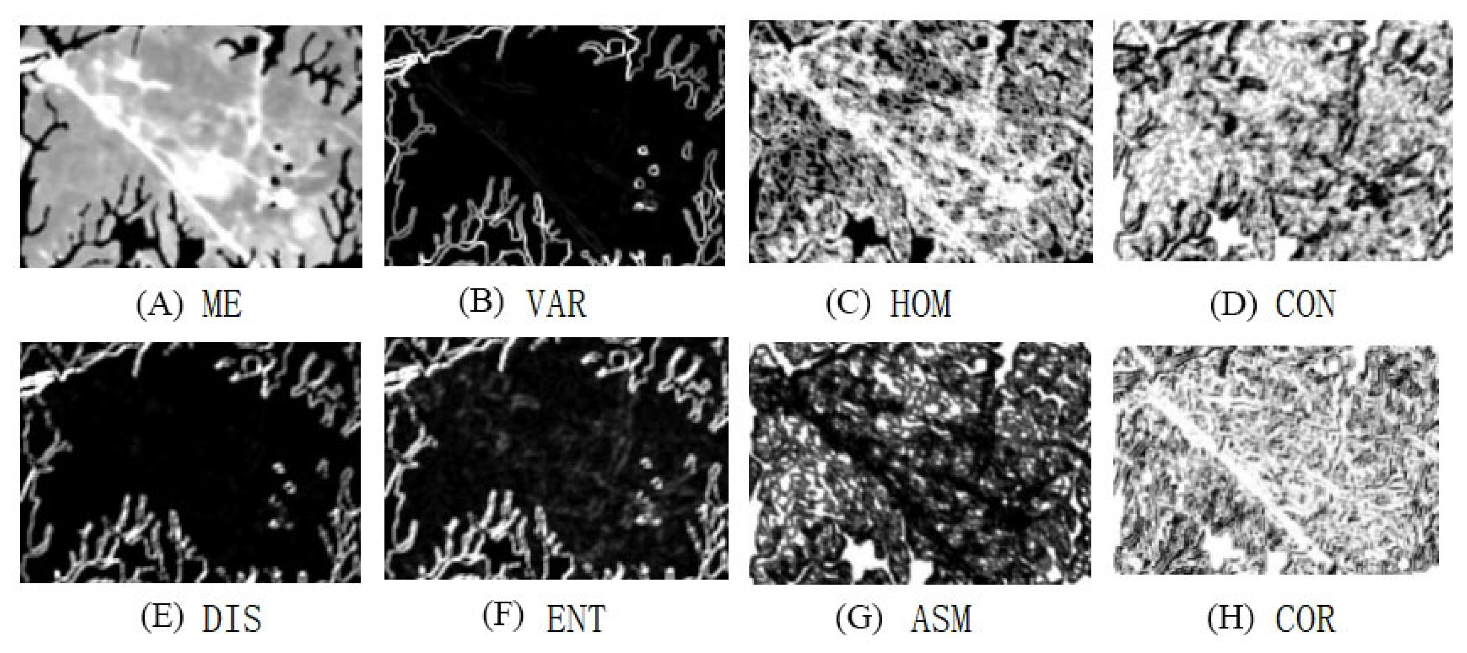
2.4.2. Extraction of Texture Feature

Earlier studies have shown that incorporating a range of texture features can effectively enhance the estimation precision of the model [38,39]. In this paper, we propose the use of a second-order statistics filter for texture feature extraction. The grey level co-occurrence matrix (GLCM) is applied after fusing the information from the GF-2 4 band and the GF-6 bands. Eight commonly used texture features are extracted, including the average (Mean), variance (Variance), contrast (Contrast), dissimilarity (Phase of the opposite sex), entropy (Information Entropy), homogeneity (Collaborative), second moment (Second Moment), and correlation (Correlation). The calculation formulas for these features are shown in

Table 4. GLCM texture feature calculation formula.

GLCM	A Formula to Calculate
ME	$Mean={\displaystyle \sum _i}{\displaystyle \sum _j}p\left(i, j\right)\ast i$
VAR	$VAR={\displaystyle \sum _i}{\displaystyle \sum _j}{ (i-u) }^{2}p\left(i, j\right)$
HOM	$HOM={\displaystyle \sum _i}{\displaystyle \sum _j}\frac{p\left(i, j\right)}{1+{ (i-j) }^2}$
CON	$CON={\displaystyle \sum _i}{\displaystyle \sum _j}{ (i-j) }^{2}p\left(i, j\right)$
DIS	$DIS={\displaystyle \sum _i}{\displaystyle \sum _j} p\left(i, j\right)\left|i-j\right|$
ENT	$ENT=-{\displaystyle \sum _i}{\displaystyle \sum _j}p\left(i, j\right)logp\left(i, j\right)$
ASM	$ASM={\displaystyle \sum _i}{\displaystyle \sum _j}{p\left(i, j\right)}^2$
COR	$COR=-{\displaystyle \sum _i}{\displaystyle \sum _j}\frac{\left(i-u_x\right)\left(j-u_y\right)}{{\sigma }_x{\sigma }_y}p (i, j)$

. The extraction windows are 3 × 3, 5 × 5, 7 × 7, 9 × 9, 11 × 11, and 13 × 13, with a moving step of 1 image element, and 64 grey levels are selected in order to avoid the influence of the window edge effect and to keep the image texture features stable and clear. The use of ENVI to extract the 8 texture feature factors under the 3 × 3 window in the 0° direction of the new red edge 1 (B5) of GF-6 is shown in Figure 5.

2.4.3. Extraction of Principal Component Characteristics

Principal component analysis (PCA) is a data dimension reduction algorithm. Dimension reduction aims to retain the most important features of high-dimensional data while removing noise and irrelevant characteristics. This helps to reduce information redundancy in multispectral images, primarily through linear transformation. PCA extracts the main information from several principal components, highlighting the most significant features. It is commonly used in transformation technology for processing multispectral remote sensing images.

Principal component analysis was performed on the information of each band of GF-2 and GF-6 images, respectively, to achieve the purpose of isolating the noise between the bands and reducing the dimension of the data set. Using forward principal component PC transform and covariance matrix for principal component analysis, the results show that the first principal component of GF-2 image contains 97.75% of the information of four bands, and the first principal component of GF-6 image contains 99.65% of the information of eight bands, which can reflect the information of each band very well.

2.4.4. Radar Images to Scattering Coefficient

The scattering coefficient refers to the unit area of radar reflectivity or the unit of radiation area on the radar scattering cross-section. In remote sensing inversion experiments, the radar scattering coefficient is typically used to express the parameters of the scattering cross-section in a given area. The parameters include the scattering intensity in the incident direction or the average radar cross section per unit area of the target. This is commonly referred to as the backward scattering coefficient. Using ENVI, the data were imported and subjected to pretreatment, including extraction, filtering, geocoding, and radiation calibration. This was carried out for two polarization modes (HH, HV) and three types of backward scattering coefficients (sigma, beta, gamma) normalized by radar brightness and incidence angle. In total, there were 6 scattering coefficients (HHsigma, HHbeta, HHgamma, HVsigma, HVbeta, and HVgamma).

2.4.5. The Terrain Factor

Based on the 30 m resolution of DEM data, the study zone can be extracted using the 3D analysis tools in ArcGIS 10.5 (Environmental Systems Research Institute, Inc., Redlands, CA, USA) to obtain terrain factors such as slope, slope direction, and altitude factor.

2.5. Model Introduction

In recent years, area-based methods have been used for various types of forest parameter estimation and have a large number of models, including parametric and non-parametric models [40,41]. Parametric models are multivariate linear and nonlinear models, and non-parametric models include machine learning methods such as artificial neural networks, support vector machines, deep learning, and regression trees [42,43]. The multivariate linear regression model is the most commonly used forest parameter estimation model in many studies [44]. In this paper, multivariate regression, random forest, and gradient-boosting decision tree algorithms were used to estimate forest carbon stocks, respectively.

2.5.1. Multiple Linear Regression (MLR)

Multiple stepwise regression is one of the classical methods of multiple regression analysis, which consists of introducing the independent variables that pass the F-statistic test into the equation one by one, and at the same time, at each step after the introduction of the third variable, the variables that have been previously introduced are tested again using the backward method, and the insignificant variables and those that have no effect on the equation are excluded, and so on until the variables can not be excluded and the new variables can not be introduced.

2.5.2. Random Forest (RF)

The random forest algorithm has good robustness and high accuracy, making it suitable for high-dimensional data sample sets. It is also high phase locked. The principle of the algorithm is based on the bootstrap method, which involves repeatedly drawing random samples from the modeling data set, taking a vote from the internal samples, and finally generating prediction results. The algorithm utilizes the random forest model and decision tree from the Python sklearn library. It involves training and constructing 50 models through repeated iterations.

2.5.3. Gradient-Boosting Decision Tree (GBDT)

Gradient-boosting decision tree (GBDT) belongs to the supervised learning algorithms in machine learning and is an iterative decision tree algorithm, a high-performance nonlinear regression prediction algorithm [45], which can also be used to implement classification tasks. The main idea lies in the gradual reduction of residuals through a continuous iterative process and the construction of multiple regression decision trees through gradient optimization. Eventually, the conclusions of all the regression trees are summarized to form the final model, which aims to simultaneously reduce the variance and bias of the model. In addition to the strong interpretability of the tree model and its ability to handle mixed models effectively, its other advantages are its strong predictive performance and excellent stability.

2.6. Accuracy Verification

The estimation results are evaluated for accuracy using the determination coefficient (R²) and root mean square error (RMSE) as evaluation indices. The calculation formula is as follows:

$$R^2=1-\frac{{\displaystyle \sum {(y_i-{\hat{y}}_i)}^2}}{{\displaystyle \sum {(y_i-{\overline{y}}_i)}^2}}$$

(1)

$$R_{mse}=\sqrt{\frac{{\displaystyle \sum {({\hat{y}}_i-y_i)}^2}}{N}}$$

(2)

Types (1) and (2): $y_i$ modeling sample biomass values, ${\widehat{y}}_i$ to sample biomass prediction, $\overline{y}$ for the sample area students average volume, N for sample number.

F and Sig values in statistics are used when building multiple linear regression equations. F value is the statistic of the F test, which is the ratio of the sum of squared deviations and degrees of freedom between and within groups. Sig in SPSS analysis is the test of significance. Sig followed by the value of Sig is the statistic of p-value, based on which a significance test is performed. If the p value 0.01 < p < 0.05, the difference is significant and if p < 0.01, the difference is highly significant.

3. Results

3.1. Data Statistics and Processing

This article selected remote sensing band data (GF-2: B1-B4; GF-6: B1-B8), vegetation index features (9), backscattering coefficients of radar images (6), principal component analysis data, and textures. Based on forest age classification, this paper applied the three standard deviations principle to eliminate outliers, and finally selected 295 data for modelling, including 130 dominant tree species of Pinus massoniana, 75 Slash pine, and 90 samples of Quercus acutissima. We randomly selected 70% of the sample data (206) as the training set for model construction, and the remaining 30% (89) as the training set for model accuracy testing. The number of modelling factors was greater than the number of modelling samples. The participation of all feature factors in modelling will increase the risk of overfitting, so it is usually necessary to select feature factors before modelling. This paper used the Pearson correlation coefficient to conduct a correlation analysis between characteristic factors and carbon storage, and it selected factors that are significantly related to carbon storage. Before correlation analysis, the data were tested for normal distribution by Q-Q plots in SPSS data analysis software (IBM SPSS Statistics v26, IBM Corp., Armonk, NY, USA).

3.2. Determination of Feature Factors

3.2.1. The Different Forest Category Correlation Analysis

The correlation coefficients between the carbon storage of multiple tree species and three single tree species and the characteristic factors of the four data sources are shown in

Table 5. Correlation between factors and carbon storage of different forest species.

	Multi-Tree Species	Correlation	Pinus massoniana	Correlation	Slash pine	Correlation	Quercus acutissima	Correlation
GF-2	pca1GF-2	0.348	pca1GF-2	0.327 **	b3_mean_5	0.489 **	band2	−0.565 **
	band1	0.364	band1	0.419 **	band 3	0.412 **	b3_mean_13	−0.625 **
	b1-mean-3	0.430	b1_mean_5	0.268 **
	b1_hom_3	−0.579	b3_hom_13	0.538 **
	b3_var_5	0.255 **	b3_var_3	−0.624 **
Terrain	SLOPE	0.325	SLOPE	0.500 **			SLOPE	0.28
	DEM	0.547 **
GF-6	MTCI	0.487 **	PCA1GF-6	−0.369 **	NDVI	0.427 **	MTCI	0.449 *
	B5_mean_13	0.540	Band6	−0.416 **	PCA1 GF-6	0.352 **	Band6	−0.502 **
	GNDVI	−0.217 *			Band4	0.405 **	GNDVI	0.376 *
							PCA1GF-6	−0.523 *
GF-3	HVgamma HVsigma	0.226 ** 0.227 **	HVsigma	0.219	HVsigma	0.225	HVgamma	0.258 *

Lowercase letters represent the feature factors of GF-2 images, and the beginning of uppercase letters represent the feature factors of GF-6 images, pca1GF-2 represents the first principal component of GF-2 image, b1-mean-3 represents the mean value of GF-2 image band 1 under a 3 × 3 window, and HVgamma represents the gamma coefficient of GF-3 image under HV polarization mode. We have shown in bold the most relevant characteristic factors for different tree species. * At the 0.05 level (two-tailed), the correlation is significant. ** At the 0.01 level (two-tailed), the correlation is significant.

.

Multi-tree species carbon stocks had the strongest correlation with b1_hom_3 of the GF-2 image, with a correlation coefficient of −0.579, and with b1-mean-3 with a correlation coefficient of 0.43, followed by band1, pca1, and B3_var_5, with correlation coefficients of 0.364, 0.348, and 0.255, respectively. The correlation coefficient of multi-species carbon stock with B5_mean_13 of GF-6 image reached 0.54, and the correlation coefficients with the vegetation indices of the new red edge band, MTCI and GNDVI, were 0.487 and −0.217, respectively. Among the six backscattering coefficients (HHsigma, HHbeta, HHgamma, HVsigma, HVbeta, and HVgamma) calculated for both GF-3 polarisation modes, only HVsigma and HVgamma showed correlation with carbon stocks, with correlation coefficients of multitree species carbon stocks with HVsigma and HVgamma were 0.227 and 0.226, respectively. The correlation coefficients of Pinus massoniana carbon stock with b3_var_3, b3_hom_13, and b1_mean_5 of GF-2 image were −0.624, 0.538, and 0.268, respectively, and the correlation coefficients of band1 and pca1 were 0.419 and 0.327; the Pinus massoniana carbon stock had the best correlation with Band6 of GF-6 image, with correlation coefficient of −0.416, and the correlation coefficient with the first principal component of GF-6 was −0.369; the HVsigma of GF-3 had a better ability to characterise the carbon stock of horsetail pine, with a correlation coefficient of 0.219. Slash pine carbon stock was better correlated with b3_mean_5 of GF-2, with a correlation coefficient of 0.489, followed by band3, with 0.412. Slash pine carbon stock was significantly correlated with normalised vegetation index (NDVI) and Band4 of GF-6, with correlation coefficients of 0.427 and 0.405, and the correlation coefficient was 0.352 with the first principal component of GF-6. The correlation coefficient of Slash pine carbon stock with HVsigma was 0.225. The correlation coefficient between the carbon stock of Quercus acutissima and b3_mean_13 of GF-2 was −0.625, with a significant negative correlation, followed by band2 with a correlation coefficient of −0.565; the first principal component of GF-6 characterised the carbon stock of Quercus acutissima better, with a correlation coefficient of −0.523, followed by the better correlation of Band6 with a correlation coefficient of −0.502; the carbon stock of Quercus acutissima was significantly correlated with the GF-6 image added red edge index MTCI and greenness vegetation index GNDVI were significantly correlated, with correlation coefficients of 0.449 and 0.376, respectively. HVgamma in the backscatter coefficients of GF-3 was correlated with Quercus acutissima carbon stock, with a correlation coefficient of 0.258. Among them, multi-tree species, Pinus massoniana and Quercus acutissima all have strong correlations with topographic factors, and the study area has an elevation of 45–385 m, so the slope has a greater effect on carbon storage. It can be seen that the correlation between the GF-2 image band texture features and GF-6 added bands as well as the new red-edge vegetation index MTCI with the multi-tree species and the three mono-species were all greater than 0.255.

3.2.2. The Different Age Group Correlation Analysis

According to the age of the forest to which the sample data belonged, the sample data were divided into young forest, middle-aged forest, near mature forest, over-mature forest and mature forest. The correlation between each factor and carbon storage of different age groups was analyzed from the perspective of different age groups, as shown in

Table 6. Correlation between factors and carbon storage in different age groups.

	Sapling Forest	Correlation	Half-Mature Forest	Correlation	Near-Mature Forest	Correlation	Over-Mature Forest	Correlation	Mature Forest	Correlation
GF-2	band3	0.256 **	band2	0.376 **	b4_mean_13	0.355 **	band1	−0.389 **	band1	−0.491 **
	b3_mean_5	0.275 **	b2_mean_5	0.275 **	band 3	0.368 **	b3_hom_13	−0.548 **	b3_var_5	−0.625 **
	b3_var_5	0.455 **	b3_cor_3	−0.593	b4_var_5	0.286			b3_mean_13	0.633
	b2_ent_3	−0.238	b3_var_3	−0.624 **
Terrain			SLOPE	0.439 **	SLOPE	0.517 **	SLOPE	0.28	SLOPE	0.28
			DEM	0.524
GF-6	SAVI	−0.53	MTCI	−0.278 **	NDREI	−0.473 **	RVI	0.468 *	B3_mean_3	0.373 *
	B2_mean_5	0.572	Band6	−0.528 **	B1_mean_3	0.527	B6_mean_3	−0.524 **	Band6	−0.488 **
	GNDVI	−0.207 *	B1_mean_13	0.326			NDREI	0.382 *	NDREI	0.397 *
	PCA1GF-6	−0.345							MTCI	−0.285 *
GF-3	HVsigma	0.215	HVsigma	0.223 **	HVgamma	0.218 **	HVgamma	0.256 *	HVgamma HVsigma	0.373 * 0.262

Lowercase letters represent the feature factors of GF-2 images, and uppercase letters represent the feature factors of GF-6 images, b3_mean_5 represents the mean value of GF-2 image band 3 under the 5 × 5 window, PCA1GF-6 represents the first principal component of GF-6 image, and HVsigma represents the sigma coefficient of GF-3 image under HV polarization mode. We show in bold the feature factors with the highest correlation for different age groups. * At the 0.05 level (two-tailed), the correlation is significant. ** At the 0.01 level (two-tailed), the correlation is significant.

.

Sapling forest carbon stocks correlate better with b3_var_5 of GF-2 image with a correlation coefficient of 0.455, followed by b3_mean_5, b2_ent_3, and band3 with correlation coefficients of 0.275, 0.256, and −0.238, respectively; the sapling forest had the best correlation with b2_mean_5 of GF-6 image with a correlation coefficient of 0.572, followed by better correlation with the soil-regulated vegetation index SAVI, the first principal component of GF-6 image, and the greenness vegetation index of GF-6 image, with correlation coefficients of −0.53, −0.345 and −0.207, respectively. Half-mature forest carbon stock was significantly correlated with b3_var_3 and b3_cor_3 of the GF-2 image, with correlation coefficients of −0.624 and −0.593, followed by better correlation with band2 and b2_mean_5, with correlation coefficients of 0.376 and 0.275, respectively. Carbon stocks in half-mature forest were significantly correlated with the added bands of GF-6 imagery, with a correlation coefficient of −0.528, followed by B1_mean_13 of GF-6 image and MTCI of GF-6 new red edge index, with correlation coefficients of 0.326 and −0.278, respectively. The carbon stock in the near-mature forest was significantly correlated with band3 of GF-2 image with a correlation coefficient of 0.368, followed by b4_mean_13 and b4_var_5 of GF-2 image, with correlation coefficients of 0.355 and 0.286, while the best correlation was found in b1_mean_3 of GF-6 image with a correlation coefficient of 0.527, followed by the new red edge vegetation index (NDREI) of GF-6 image, with a correlation coefficient of −0.473. Carbon stocks in the over-mature forest were significantly correlated with b3_hom_13 of GF-2 image with a correlation coefficient of −0.548, followed by band1 with a better correlation coefficient of −0.389; the best correlation was with B6_mean_3 of GF-6 image, with a correlation coefficient of −0.524, followed by a significant correlation with the ratio vegetation index RVI and GF-6, added respectively. The red edge vegetation index NDREI had correlation coefficients of 0.468 and 0.382, respectively. Mature forest carbon stock correlated well with b3_mean_13 and b3_var_5 of GF-2 image, with correlation coefficients of 0.633 and −0.625, respectively, and band1 of GF-2 image also correlated significantly with mature forest carbon stock, with a correlation coefficient of −0.491. Mature forest carbon stock correlated significantly with the new band of GF-6 image, with a correlation coefficient of −0.488, followed by the new red edge vegetation index NDREI and MTCI, and B3_mean_3 with correlation coefficients of −0.488, respectively. The correlation coefficients were 0.397, −0.285, and 0.373 for the new red edge vegetation index NDREI and MTCI and B3_mean_3 of the GF-6 image, respectively. The two backscattering coefficients HVsigma and HVgamma in the HV polarization mode of the GF-3 image showed good correlation with the carbon stock of mature forests, with correlation coefficients of 0.262 and 0.373, respectively; the carbon stock of the sapling forest and half-mature forest showed good correlation with the HVsigma of the GF-3 image, and the carbon stock of the near-mature forest and over-mature forests showed significant correlation with the HVgamma of the GF-3 image. The carbon stocks in near-mature forest and over-mature forests were significantly correlated with HVgamma of GF-3 images. In addition, the slope orientation factor among the topographic factors had a strong correlation with the carbon stocks of different age groups, and the most significant correlation coefficient with the carbon stocks of near-mature forests reached 0.517.

3.3. Analysis of Modeling Results of Different Images

This process continued until no further variables could be eliminated or introduced. The application of multiple stepwise regression models was performed on two single optical data sets, joint optical data, and joint optical data combined with radar data. The four species were categorized into three main tree species, and models were constructed for the entire forest tree population. The application of SPSS to build multiple stepwise linear regression models, combined with collinearity diagnosis, was used to factor into the model for further screening and ensure the accuracy of the regression model.

Four types of forests, including Pinus massoniana, Slash pine, and multiple tree species (Quercus acutissima), were used to develop a carbon fitting regression equation. The model’s R², RMSE (t/ha), and F value are shown in

Table 7. Multiple stepwise regression modeling results of different tree species.

Multi-Tree Species		R2	RMSE (t/ha) /(t·hm−2)	F	Sig
GF-2	AGC = 0.128 × DEM + 0.267 × pca1 − 2.107 × b1_hom_3 −+ 12.457 × band1 + 4362.039	0.465	30.78	67.536	0
GF-6	AGC = 468.056 × MTCI + 1.576 × SLOPE + 14.826 × B5_mean_13 − 1.543 × GNDVI + 537.297	0.429	30.12	58.673	0
GF-2&GF-6	AGC = 1013.454 × MTCI + 1.683 × SLOPE + 561.873 × GNDVI + 0.263 × DEM + 7693.412 × b1_mean_3 − 0.42 × b3_var_5 + 542.861	0.538	28.01	51.498	0
GF-2&GF-6&GF-3	AGC = 824.31 × DEM + 3.586 × SLOPE + 482.16 × MTCI + 692.43 × b1_hom_3 ++ 0.23 × HV_sigma + 0.56 × HV_gamma + 592.432	0.649	25.14	46.489	0
Pinus massoniana
GF-2	AGC = 4.13 × SLOPE + 0.547 × b3_var_3 − 2.357 × b3_hom_13 − 84.93 × band1 + 2315.364	0.514	17.25	38.279	0
GF-6	AGC = −5.384 × SLOPE − 2.548 × Band6 − 1.026 × PCA1 + 42.513	0.327	29.53	25.974	0
GF-2&GF-6	AGC = 5.317 × SLOPE + 6.482 × Band6 − 0.027 × PCA1 + 0.725 × b3_var_3 + 634.825 × b3_hom_13 + 516.089	0.589	16.29	34.171	0
GF-2&GF-6&GF-3	AGC = 3.574 × SLOPE + 1.035 × PCA1 − 13.541 × b3_var_3 − 1.164 × Band6 + 128.49 × band1 + 0.063 × HVsigma + 504.196	0.614	12.28	30.562	0
Slash pine
GF-2	AGC = 0.057 × b3_mean_5 + 135.27 × band3 + 128.574	0.372	13.35	19.273	0
GF-6	AGC = 154.29 × NDVI − 1.569 × PCA1 + 3.67 × Band4 + 328.154	0.294	14.12	11.157	0
GF-2&GF-6	AGC = 0.058 × Band4 + 153.47 × b3_mean_5 + 0.027 × band3 + 159.262	0.405	14.01	15.147	0
GF-2&GF-6&GF-3	AGC = 1.472 × band3 + 0.013 × b3_mean_5 − 128.251 × PCA1 + 275.13 × NDVI + 0.254 × HVsigma + 783.45	0.496	13.23	9.174	0
Quercus acutissima
GF-2	AGC = 0.218 × SLOPE + 1.517 × band2−11.974 × b3_mean_13 + 1047.17	0.521	42.07	18.138	0
GF-6	AGC = 894.271 × MTCI − 20.15 × PCA1 + 1182.3 × Band6 + 138.2	0.584	32.56	23.384	0
GF-2&GF-6	AGC = 681.29 × MTCI−0.35 × band2 − 0.272 × Band6 + 774.15 × b3_mean_13 + 579.24	0.612	29.71	21.147	0
GF-2&GF-6&GF-3	AGC = 0.013 × GNDVI + 134.56 × MTCI − 0.21 × band2 − 32.54 × PCA1 + 115.32 × b3_mean_13 + 0.258 × HVgamma + 514.067	0.659	27.09	20.573	0

Lowercase letters represent the feature factors of GF-2 images, and beginning of uppercase letters uppercase letters represent the feature factors of GF-6 images.

. For the four classes, the optimal fitting R² values were 0.649, 0.614, 0.496, and 0.659, respectively, for the joint optical and radar data model fitting results. Secondly, the use of two types of optical data resulted in higher fitting precision compared to using only a single type of optical data. When considering a single type of optical data, the modelling results for multiple tree species, horsetail pine, and Slash pine using GF2 data were better than those using GF6 data. The goodness of fit for GF2 modelling results were 0.465, 0.514, 0.372, and 0.521, respectively, while the GF-6 modelling results were 0.429, 0.327, and 0.294. Furthermore, the modelling results for Quercus acutissima using GF data were better than those using GF2 and GF6 data, with an R² value of 0.584 and 0.521, respectively.

3.4. Modeling Analysis on Different Models for Mixed Forest

The precision of fitting multiple tree species in a stepwise regression model is low. Therefore, we introduced random forests and gradient-boosting decision tree algorithms to explore different models for improving the accuracy of carbon modeling for multiple tree species. We compared two different integration approaches to assess the applicability of carbon reserve estimation algorithms. This study selected the strong correlation between carbon and multiple tree species, as well as six variables (SLOPE, DEM, MTCI, b1_hom_3, HV_sigma, and HV_gamma), as the main factors for forest carbon modeling.

3.4.1. Random Forest Algorithm

In this paper, the implementation of model construction was carried out in Python 2.7(CNRI, Virginia, United States) language, applying pycharm editor for code writing and calling the random forest model in sklearn to achieve model construction. After several adjustments to the parameters, the highest model accuracy was established after the ntree was 475 and the m-value was set to 100; the test set was output and the model accuracy was evaluated; the RMSE function was called to evaluate the model fitting results and the accuracy of the predicted data; the prediction results were outputted and the graphs were generated.

3.4.2. Gradient Promotion Decision Tree

The process of calculating using the additive model, known as GBDT, is shown below:

Model input: Training set $T=\left\{\right(x_1,y_1),(x_2,y_2),\dots ,(x_{N }, y_{N }\left)\right\},x_{i }\in \mathrm{X}\subseteq R^n,y_{i }\in Y\subseteq R;\mathrm{L}\mathrm{o}\mathrm{s}\mathrm{s} \mathrm{f}\mathrm{u}\mathrm{n}\mathrm{c}\mathrm{t}\mathrm{i}\mathrm{o}\mathrm{n} L(y , f(x\left)\right)$

Model output: GBDT Model $\widehat{f} \left(x\right)$

Model process:

(1)

Initialize

$$f_0 \left(x\right)={arg}_{\theta }min\sum _{i=1}^{N}L (y_i; \theta )$$

(3)

(2)

To $m=1,2,\dots ,M$

(a)

To $i=1,2,\dots ,N$, calculate

$$r_{mi}=-[\frac{\partial L(y_i,f(x\left)\right)}{\partial f\left(x_i\right)}{]}_{f\left(x\right)=f_{m-1}\left(x\right)}$$

(4)

That is, the negative gradient of each sample loss function is used as an approximation of the sample residual $r_{mi}=y_i-f \left(x_i\right)$.

(b)

$r_{mj}$ is fitted into a CART and set of leaf nodes is obtained $R_{mj}$, j = 1, 2, …, J.

(c)

To $j=1 ,2, \dots ,J$, find the minimized loss function:

$${\theta }_{mj={arg}_{\theta }min}\sum _{x_{i\in R_{mj}}}L (y_{i , f_{m-1}}(x_i)+\theta )$$

(5)

(d)

Update forecast results:

$$f_m \left(x\right)=f_{m-1} \left(x\right)+\sum _{j=1}^J{\theta }_{mj}I (x \in R_{mj})$$

(6)

(3)

The GBDT model is obtained:

$$\widehat{f}=f_M \left(x\right)=\sum _{m=1}^M\sum _{j=1}^J{\theta }_{mj}I (x\in R_{mj})$$

(7)

In the formula, N is the number of samples, M represents the number of regression trees, J represents the number of leaf nodes in the regression tree, I(x) represents the indicator function used to judge the elements in the collection, and also represents the override parameter.

Note that the model regression plot is shown in Figure 6.

The estimation results show that the random forest and gradient-boosting decision tree algorithms have good fitting results for estimating the carbon storage of multiple tree species. The accuracy of the verification sample has been verified. The coefficient of determination (R²) and root mean square error (RMSE) were used to test whether there is a good fitting effect between the predicted value and the measured value of the model. As shown in Figure 6: A, B, and C are the fitting effects of multiple stepwise regression, random forest, and gradient-boosting decision tree algorithm training samples, respectively; a, b, and c are, respectively, multiple stepwise regression, random forest, and gradient boosting. The decision tree verifies the fitting effect of the sample. It can be seen that gradient-boosting decision tree has the best fitting effect, with R² reaching 0.902 and RMSE being 10.261 t/ha; random forest comes second, with R² reaching 0.824 and RMSE being 16.853 t/ha; and multiple stepwise regression has the worst fitting effect, with R² reaching 0.636 and an RMSE of 29.948 t/ha. In the verification sample, the gradient-boosting decision tree and random forest models performed relatively stably, and the R² and RMSE of the models were both higher than the predicted results.

3.5. Distribution Map of Carbon Storage Estimation Results

Based on the estimation of the three main tree species of Pinus massoniana, Slash pine, and Quercus acutissima in the forest area, the remaining few tree species in the forest area were treated as broad-leaved mixed forests. For these four forest stand types, carbon storage distribution mapping was carried out based on the estimation results of carbon storage using multiple stepwise regression, random forest, and GBDT models.

Figure 7 shows the spatial distribution of forest carbon storage in Huangfu Mountain. Carbon storage values range from 0.115 t/ha to 166.067 t/ha. The estimation results of the multiple stepwise regression algorithm are generally low. The difference in the estimation results of the random forest and gradient-boosting decision tree models is mainly concentrated in the low-value part. The random forest algorithm is too low for estimating the low-value part, so the gradient-boosted decision tree (GBDT) algorithm is better for estimating the low-value region. The estimation effect of carbon storage in high-value areas is better. The two models have better estimation effects on carbon storage in high-value areas. The medium- and high-value areas of the three models are all distributed in the central forest area.

4. Discussion

In this study, we extracted spectral information, texture features, radar coefficients, and topographic data of GF-2, GF-6, and GF-3 images as feature factors. We examined different tree species and measured carbon in different age groups, considering the characteristic factor of close sex. The research found that GF-2 image texture features showed a good correlation with previous studies, indicating that they can improve the forecast precision measurements of volume and forest biomass [46,47].

The GF-6 image of the new red edge band and its derivative of the vegetation index show a high correlation with the measured carbon. This echoes the highest correlation between MTCI constructed from the GF-6 image red edge index and measured biomass obtained by Jiang et al. [48]. However, the correlation coefficients in this paper are slightly lower than the results of Jiang et al. This may be due to the fact that the study area in this paper has a natural secondary forest, contrary to the plantation in the study area of Jiang et al. [49]. Additionally, this article only utilizes GF-3 images with fine banding data, specifically, the HH and HV polarization modes. The analysis only yielded a correlation between the sigma and gamma coefficients in the HV polarization mode of the GF-3 image. Future considerations include the use of polarization band radar data. All unused backscatter systems should be joined for analysis.

Based on multiple stepwise regression decision tree models, this study introduces random forests and gradient estimates of carbon for multiple tree species. The aim is to compare two different integrations and assess the applicability of the method in regression prediction problems. The estimation results of the random forest show an R² value of 0.871, while the gradient of the decision tree for estimating results shows an R² value of 0.902. This study, along with previous studies on gradient promotion decision trees for nonlinear regression problems, demonstrates better applicability and consistent conclusions compared to random forests.

Given the limited use of sample data, the analysis of the Pearson correlation coefficient in this study only examines the characteristics of different tree species with more factors. It does not consider the carbon responsiveness of the same age group or estimate carbon reserves in a single tree species and the same age group. Follow-up studies will expand the number of test samples and provide carbon age estimates for tree forests from the perspective of different tree species and age groups.

The future trend will involve using multi-source remote sensing data as the primary data source and selecting the appropriate machine learning and deep learning algorithms for estimating carbon inversion. This paper only compares the decision trees of these two kinds of random forests, and for the gradient degree of machine learning methods in the applicability of the regression prediction problem, the precision is high and low. Subsequent studies will join carbon reserve estimation by the deep degree algorithm, further exploring the applicability of different algorithms for carbon remote sensing estimation. Meanwhile, in this paper, only the coefficient of determination (R²) and the root mean square error (RMSE) were chosen as the evaluation indexes to represent the carbon stock estimation model, and in subsequent research, we can consider adding indicators such as the mean absolute percentage error (MAPE), the Akaike information criterion (AIC), and the Bayesian information criterion (BIC) to construct a system to evaluate the carbon stock estimation model, to enhance the reliability and applicability of the research results.

5. Conclusions

In this study, we combined multi-satellite data and analyzed the characteristic factors significantly related to carbon storage in Huangfu Mountain National Forest Park. The study reached the following conclusions:

• The texture characteristics of the GF-2 image, the new band and the new red edge vegetation index of the GF-6 image, the radar intensity coefficient sigma, and the radar brightness coefficient beta of the HV polarization mode under the refined strip of the GF-3 image and forest carbon storage have good responsiveness;
• Regarding different forest species, Pinus massoniana carbon reserves have the best correlation with the new red edge band of GF-6 images; Slash pine carbon reserves have the best correlation with texture features of GF-2 images; Quercus acutissima carbon reserves have the best correlation with textural features of GF-2 images and new red edge index MTCI and greenness vegetation index GNDVI of GF-6 images; and the slope has a greater impact on the carbon storage of multiple tree species and single tree species, Pinus massoniana and Quercus acutissima. For different age groups, the carbon storage of sapling forests, half-mature forest, over-mature forests, and mature forests all have a high correlation with the texture characteristics of GF-2 images. Half-mature forests’, near-mature forests’ and over-mature forests’ carbon storage is also significantly correlated with the new bands of GF-6 images; there is a good correlation between carbon storage in sapling forests and half-mature forests and the sigma coefficient in the HV polarization mode of GF-3 images; near-mature forests’ and over-mature forests’ carbon storage is significantly correlated with the gamma coefficient under the HV polarization mode of GF-3 images; in addition, the slope aspect factor in the terrain factors has a strong correlation with the carbon storage of different age groups.
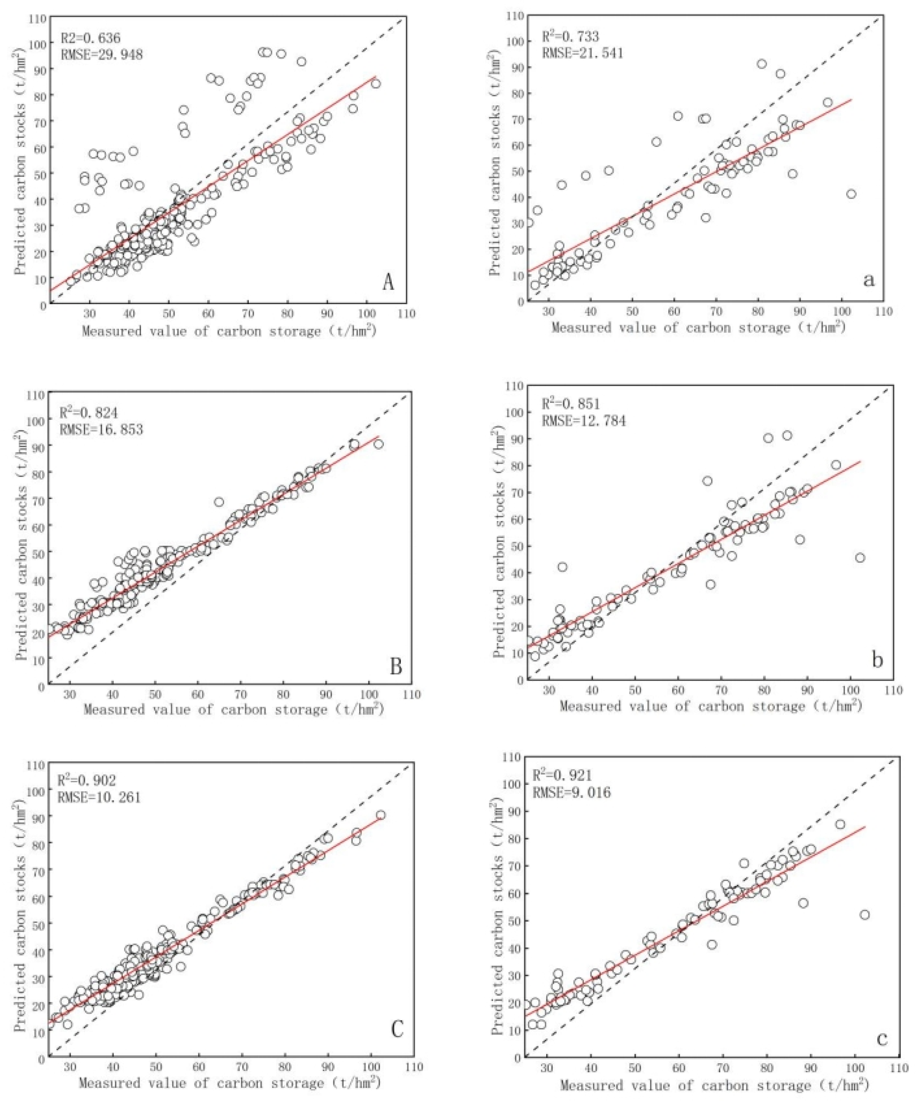
• On the basis of the traditional regression algorithm, multivariate stepwise regression, the random forest, and gradient-boosting decision tree models are introduced into multi-tree species modeling. The results show that among the two different integrated thinking algorithms, gradient-boosting decision tree has a higher estimation accuracy and the fitting effect is better than that of random forest; R² reaches 0.902, RMSE is 10.261 t/ha; random forest is second; R² reaches 0.824, RMSE is 16.853 t/ha; and multiple stepwise regression has the worst fitting effect; R² reaches 0.636, RMSE is 29.948 t/ha.

References

1. Kuuluvainen, T.; Gauthier, S. Young and old forest in the boreal: Critical stages of ecosystem dynamics and management under global change. For. Ecosyst. 2018, 5, 361–375. [Google Scholar] [CrossRef]
2. Zhao, M.; Yang, J.; Zhao, N.; Liu, Y.; Wang, Y.; Wilson, J.P.; Yue, T. Estimation of China’s forest stand biomass carbon sequestration based on the continuous biomass expansion factor model and seven forest inventories from 1977 to 2013. For. Ecol. Manag. 2019, 448, 528–534. [Google Scholar] [CrossRef]
3. FAO. State of the World’s Forests 2011; FAO: Rome, Italy, 2011; p. 179. [Google Scholar]
4. FAO. Global Forest Resources Assessment 2015—How Are the World’s Forests Changing, 2nd ed.; FAO: Rome, Italy, 2016; p. 54. [Google Scholar]
5. Dixon, R.K.; Solomon, A.M.; Brown, S.; Houghton, R.A.; Trexier, M.C.; Wisniewski, J. Carbon pool and flux of global forest ecosystems. Science 1994, 263, 185–190. [Google Scholar] [CrossRef] [PubMed]
6. Su, R.; Du, W.; Ying, H.; Shan, Y.; Liu, Y. Based on LiDAR and multi-spectral images of forest land carbon reserves estimation: Du, coniferous forest, for example. Forests 2023, 14, 992. [Google Scholar] [CrossRef]
7. Kan, Y.; Han, Z.; Huang, G.; Wang, X.; Li, Y.; Zhou, J.; Dian, Y. Forest biomass inversion of north subtropical zone based on high-resolution remote sensing image. J. Ecol. 2021, 41, 2161–2169. [Google Scholar]
8. Yu, G.; Chen, Z.; Piao, S.; Peng, C.; Ciais, P.; Wang, Q.; Li, X.; Zhu, X. High carbon dioxide uptake by subtropical forest ecosystems in the East Asiam monsoon region. Proc. Natl. Acad. Sci. USA 2014, 111, 4910–4915. [Google Scholar] [CrossRef] [PubMed]
9. Wen, D.; He, N.P. Forest carbon storage along the north south transect of eastern China: Spatial patterns, allocation, and influencing factors. Ecol. Indic. 2016, 61, 960–967. [Google Scholar] [CrossRef]
10. Ma, C.; Zhao, M.; Mou, H.; Liu, B. The yanshan mountains in north China larch plantation carbon density and distribution characteristics. J. Soil Water Conserv. Sci. 2017, 31, 208–214. [Google Scholar]
11. Cheng, J.; Lee, X.; Theng, B.K.; Zhang, L.; Fang, B.; Li, F. Biomass accumulation and carbon sequestration in an age sequence of Zanthoxylum bungeanum plantations under the Grain for Green Program in karst regions, Guizhou Province. Agric. For. Meteorol. 2015, 203, 88–95. [Google Scholar] [CrossRef]
12. Zhu, J.; Hu, H.; Tao, S.; Chi, X.; Li, P.; Jiang, L.; Ji, C.; Zhu, J.; Tang, Z.; Pan, Y.; et al. Carbon stocks and changes of dead organic matter in China’s forests. Nat. Commun. 2017, 8, 151–160. [Google Scholar] [CrossRef]
13. Cui, Y.; Sun, H.; Wang, G.; Li, C.; Xu, X. A Probability-based spectral unmixing analysis for percentage vegetation cover of arid and semi-arid areas. Remote Sens. 2019, 11, 3038. [Google Scholar] [CrossRef]
14. Hu, Y.; Xu, X.; Wu, F.; Sun, Z.; Xia, H.; Meng, Q.; Huang, W.; Zhou, H.; Gao, J.; Li, W.; et al. Estimating forest stock volume in Hunan province, China, by integrating in situ plot data, sentinel-2 images, and linear and machine learning regression models. Remote Sens. 2020, 12, 186. [Google Scholar] [CrossRef]
15. Sinha, S.; Jeganathan, C.; Sharma, L.K.; Nathawat, M.S. A review of radar remote sensing for biomass estimation. Int. J. Environ. Sci. Technol. 2015, 12, 1779–1792. [Google Scholar] [CrossRef]
16. Li, L.; Chen, E.; Li, Z.; Chong, R.; Zhao, L.; Gu, X. Forest aboveground biomass of InSAR baseline tomographic method estimates. Sci. Silvae Sin. 2017, 53, 85–93. [Google Scholar]
17. Liu, X.; Sui, C.; Bai, Y.; Zhao, D.; Zhao, Y.; Liu, Y.; Zhai, Q. Ground-based lidar scrub grassland lobular caragana biomass estimation. J. Remote Sens. 2020, 24, 894. [Google Scholar] [CrossRef]
18. Qiu, S.; Xing, Y.; Xu, W.; Ding, J.; Tian, J. Spaceborne large flare LiDAR with HJ-1 a hyperspectral data to estimate the regional forest biomass on the ground. Acta Ecol. Sin. 2016, 4, 7401–7411. [Google Scholar]
19. Wang, X.; Guo, Y.; He, J. Based on HJ1B and ALOS/PALSAR data of forest aboveground biomass remote sensing estimation. Acta Ecol. Sin. 2016, 4, 4109–4121. [Google Scholar]
20. Jiao, Y.; Wang, D.; Yao, X.; Wang, S.; Chi, T.; Meng, Y. Forest Emissions Reduction Assessment Using Optical Satellite Imagery and Space LiDAR Fusion for Carbon Stock Estimation. Remote Sens. 2023, 15, 1410. [Google Scholar] [CrossRef]
21. Lu, D.; Chen, Q.; Wang, G.; Moran, E.; Saah, D. Aboveground forest biomass estimation with Landsat and LiDAD data and uncertainty analysis of the estimates. Int. J. For. Res. 2012, 2012, 1–17. [Google Scholar] [CrossRef]
22. Chen, Q.; Qi, C. Lidar remote sensing of vegetation biomass. Remote Sens. Nat. Resour. 2013, 399, 399–420. [Google Scholar]
23. Eckert, S. Improved forest biomass and carbon estimations using texture measures from World View-2 satellite data. Remote Sens. 2012, 4, 810–829. [Google Scholar] [CrossRef]
24. Imhoff, M.L. Radar backscatter and biomass saturation: Ramifications for global biomass inventory. IEEE Trans. Geosci. Remote Sens. 1995, 33, 511–518. [Google Scholar] [CrossRef]
25. Boyd, D.S.; Foody, G.M.; Curran, P.J. The relationship between the biomass of Cameroonian tropical forests and radiation reflected in middle infrared wavelengths. Int. J. Remote Sens. 1999, 20, 1017–1023. [Google Scholar] [CrossRef]
26. Shen, X.; Cao, L.; She, G. Subtropical forest biomass estimation based on hyperspectral and high-resolution remotely sensed date. Remote Sens. 2016, 20, 1446–1460. [Google Scholar]
27. Huang, K.; Pang, Y.; Shu, Q.; Fu, T. Aboveground forest biomass estimation using ICESat GLAS in Yunnan, China. Remote Sens. 2013, 17, 165–179. [Google Scholar]
28. Ahmed, M.M.; Abdel-Aty, M. Application of stochastic gradient boosting technique to enhance reliability of real-time risk assessment: Use of automatic vehicle identification and remote traffic microwave sensor data. Transp. Res. Rec. 2018, 2386, 26–34. [Google Scholar] [CrossRef]
29. Zhang, Y.; Zhang, R.; Ma, Q.; Wang, Y.; Wang, Q.; Huang, Z.; Huang, L. A feature selection and multi-model fusion-based approach of predicting air quality. ISA Trans. 2020, 100, 210–220. [Google Scholar] [CrossRef]
30. Elith, J.; Leathwick, J.R.; Hastie, T. A working guide to boosted regression trees. J. Anim. Ecol. 2008, 77, 802–813. [Google Scholar] [CrossRef]
31. Cheng, B.; Liang, C.; Liu, X.; Liu, Y.; Ma, Y.; Wang, G. Research on a novel extraction method using Deep Learning based on GF-2 images for aquaculture areas. Int. J. Remote Sens. 2020, 41, 3575–3591. [Google Scholar] [CrossRef]
32. Xu, X.; Zhang, D.; Hou, X.; Ma, X.; Wang, J. Orthorectification of high-resolution remote sensing images using Google Earth and SRTMGL1. Surv. Mapp. Bull. 2018, 8, 62–67. [Google Scholar] [CrossRef]
33. Sun, M. Research on Satellite Remote Sensing Inversion Method for Forest Carbon Stock in Beijing. Master’s Thesis, Beijing Forestry University, Beijing, China, 2017. [Google Scholar]
34. Wang, Z. Research on Spatial and Temporal Changes of Forest Carbon Stock and Influencing Factors in Hangzhou Based on CASA Model. Master’s Thesis, Zhejiang Agriculture and Forestry University, Hangzhou, China, 2021. [Google Scholar]
35. Zhang, G. Spatial distribution characteristics of urban forest carbon stock in Shanghai based on remote sensing estimation. J. Ecol. Environ. 2021, 30, 1777–1786. [Google Scholar]
36. Zheng, Y.; Wu, B.; Zhang, M. Sentinel-2 data of winter wheat on dry biomass estimation and evaluation. J. Remote Sens. Sci. 2017, 21, 318–328. [Google Scholar]
37. Dash, J.; Curran, P.J. Evaluation of the MERIS terrestrial chlorophyll index (MTCI). Adv. Space Res. 2007, 39, 100–104. [Google Scholar] [CrossRef]
38. Liu, Q.; Yang, L.; Liu, Q.; Li, J. Review of forest above ground biomass inversion methods based on remote sensing technology. J. Remote Sens. 2015, 19, 62–74. [Google Scholar]
39. Bu, X.; Dong, S.; Mi, W.; Li, F. Spatial-temporal change of carbon storage and sink of wetland ecosystem in arid regions, Ningxia Plain. Atmos. Environ. 2019, 204, 89–101. [Google Scholar]
40. Dalla Corte, A.P.; Souza, D.V.; Rex, F.E.; Sanquetta, C.R.; Mohan, M.; Silva, C.A.; Zambrano, A.M.A.; Prata, G.; de Almeida, D.R.A.; Trautenmüller, J.W.; et al. Forest inventory with highdensity UAV-Lidar: Machine learning approaches for predicting individual tree attributes. Comput. Electron. Agric. 2020, 179, 105815. [Google Scholar] [CrossRef]
41. Coops, N.C.; Tompalski, P.; Goodbody, T.R.; Queinnec, M.; Luther, J.E.; Bolton, D.K.; White, J.C.; Wulder, M.A.; van Lier, O.R.; Hermosilla, T. Modelling lidarderived estimates of forest attributes over space and time: A review of approaches and future trends. Remote Sens. Environ. 2021, 260, 112477. [Google Scholar] [CrossRef]
42. Xu, G.; Manley, B.; Morgenroth, J. Evaluation of modelling approaches in predicting forest volume and stand age for smallscale plantation forests in New Zealand with Rapid Eye and LiDAR. Int. J. Appl. Earth Obs. Geoinf. 2018, 73, 386–396. [Google Scholar]
43. Zhang, L.; Shao, Z.; Liu, J.; Cheng, Q. Deep learning based retrieval of forest aboveground biomass from combined LiDAR and landsat 8 data. Remote Sens. 2019, 11, 1459. [Google Scholar] [CrossRef]
44. Vauhkonen, J.; Maltamo, M.; McRoberts, R.E.; Næsset, E. Introduction to forestry applications of airborne laser scanning. In Forestry Applications of Airborne Laser Scanning-Concepts and Case Studies; Springer: Amsterdam, The Netherlands, 2014; pp. 1–16. [Google Scholar]
45. Han, Q.; Zhang, X.; Shen, W. Lithology identification technology based on gradient boosting decision tree (GBDT) algorithm. Bull. Mineral. Petrol. Geochem. 2018, 37, 1173–1180. [Google Scholar]
46. Xiao, Y.; Xu, X.; Long, J.; Lin, H. Based on the domestic high marks data of forest volume inversion study. For. Resour. Manag. 2021, 3, 101–107. [Google Scholar]
47. Gou, R.; Chen, J.; Duan, G.; Yang, R.; Pu, Y.; Zhao, J.; Zhao, P. Biomass of pinus tabulaeformis plantation the ground inversion based on GF-2. J. Appl. Ecol. 2019, 30, 4031–4040. [Google Scholar]
48. Jiang, F.; Sun, H.; Li, C.; Ma, K.; Chen, S.; Long, J.; Ren, L. Retrieving the forest aboveground biomass by combing the red edge bands of Sentinel-2 and GF-6. Acta Ecol. Sin. 2021, 41, 8222–8236. [Google Scholar]
49. Xiong, H.; Yu, F.; Gu, X.; Wu, X. Biomass, net production, carbon storage and spatial distrubution features of different forest vegetation in Fanjing Mountains. Ecol. Environ. Sci. 2021, 30, 264–273. [Google Scholar]
Figure 1. Location of the study area. (a) the study area in Anhui Province, (b) Chuzhou City, (c) the Huangfu Mountain National Forest Park.
Forests 14 02388 g001
Figure 2. Flow chart.
Forests 14 02388 g002
Figure 3. Single band information of optical image ((a) is the surface reflectance of band 1 of the GF-2 image, (b) is the surface reflectance of band 2, (c) is the surface reflectance of band 3, and (d) is the surface reflectance of band 4).
Forests 14 02388 g003
Figure 4. Vegetation index extraction results ((A) is the calculated normalized vegetation index (NDVI), (B) is the enhanced vegetation index (EVI), (C) is the differential vegetation index (EVI), (D) is the ratio vegetation index (RVI), (E) is the soil-regulated vegetation index (SAVI), (F) is the infrared percentage vegetation index (IPVI), and (G) is the MTCI vegetation index. (H) is the green normalized vegetation index (GNDVI), and (I) is the NDREI vegetation index).
Forests 14 02388 g004
Figure 5. Optical image texture feature extraction results ((A) is the extraction result of mean value (ME), (B) is the extraction result of variance (VAR), (C) is the extraction result of homogeneity (HOM), (D) is the extraction result of contrast (CON), (E) is the extraction result of dissimilarity (DIS), (F) is the extraction result of entropy (ENT), and (G) is the extraction result of second-order moment (ASM). (H) is the extraction result of correlation (COR)).
Forests 14 02388 g005
Figure 6. Estimation results and verification of different models and multiple tree species (AC), carbon storage prediction results of multi-source stepwise regression, random forest and gradient lifting decision tree models; (ac) carbon storage verification results of multi-source stepwise regression, random forest and gradient lifting decision tree models. The straight line in the figure is a 1:1 standard line, the circles represent the input true and predicted values, and the red line is the fitted curve based on the true and predicted values.
Forests 14 02388 g006
Figure 7. The distribution of carbon storage estimation results for different models. (a) Multiple regression carbon storage estimation results, (b) random forest carbon stock estimation results, (c) GBDT carbon stock estimation results.
Forests 14 02388 g007