Article

The Performance of Discriminative Tracking Algorithms for the Sway Frequency Measurement of Betula platyphylla Sukaczev (Individual Branch and Tree) under Artificial and Natural Excitation

1
College of Computer and Control Engineering, Northeast Forestry University, Harbin 150040, China
2
College of Electrical and Information Engineering, Heilongjiang University of Technology, Jixi 158100, China
*
Author to whom correspondence should be addressed.
Forests 2023, 14(11), 2196; https://doi.org/10.3390/f14112196
Submission received: 15 September 2023 / Revised: 20 October 2023 / Accepted: 2 November 2023 / Published: 4 November 2023
(This article belongs to the Section Forest Inventory, Modeling and Remote Sensing)

Abstract

:
The sway frequency is an important component of the dynamic characteristics of trees. Video-based methods can be used to measure the sway frequencies of trees. The key to successfully measuring tree sway frequency using video methods lies in whether the tracking method employed is appropriate. Based on six algorithms, i.e., Boosting, TLD, MIL, KCF, MOSSE and CSR-DCF, the tracking performance and accuracy of tree sway frequency measurements were investigated under two conditions: artificial excitation and environmental excitation. The results show that the following: (1) In terms of the tracking speed of tree sway, MOSSE > KCF > CSR-DCF > Boosting > MIL > TLD. (2) The TLD algorithm is not suitable for tree sway tracking. Boosting, MIL, MOSSE, KCF and CSR-DCF can be used for tree sway tracking. (3) Boosting, MIL and MOSSE are suitable for measuring the sway frequency of artificially excited branches and environmentally excited trees. (4) KCF and CSR-DCF algorithms are not suitable for the measurement of branch sway frequency under artificial excitation conditions but can be used for the measurement of tree sway frequency under environmental excitation conditions. However, it should be noted that this experiment only takes a Betula platyphylla Sukaczev tree and a Betula platyphylla Sukaczev branch as the research object to verify the effectiveness and feasibility of each tracking method, and does not verify the generalization ability of the above methods (on multiple tree species and multiple trees).

1. Introduction

Wind has a significant impact on individual trees or entire forest stands, and it is one of the main causes of forest disasters. In strong winds, trees may break or be uprooted due to excessive wind load [1,2], resulting in a decrease in timber production and causing economic losses [3,4,5]. Tree sway frequency is an important part of the dynamic characteristics of trees. When the tree reaches its fundamental sway frequency, the amplitude of its sway rapidly increases, resulting in damage and destruction of the tree [6,7]. In addition, branches have a significant impact on the dynamic properties of trees. The overall damping of a tree depends on the elastic modulus and natural frequency of its branches [8]. For multiple resonance damping in trees, the natural frequencies of the branches are close to the natural frequency of the entire tree [9]. Therefore, measuring the natural frequencies of individual branches is of great significance in studying the overall multiple resonance damping motion of trees. In conclusion, it is necessary to measure the fundamental sway frequencies of both the entire tree and individual branches.
In order to measure the fundamental sway frequencies of trees, it is necessary to induce the sway motion of trees using external forces. There are two types of excitation methods depending on the source of excitation. One type is in windless conditions where artificial forces such as ropes, vibrators, and hammers are used to provide excitation [10,11,12]. The other type is in natural conditions, where the excitation is naturally provided by wind. Among them, artificial excitation can quickly determine the fundamental sway frequency of trees in a short time. On the other hand, natural wind excitation requires long-term monitoring of trees. After the tree is excited to sway, the fundamental sway frequency of the tree can be measured using two methods: contact-based and non-contact-based methods. Contact-based methods include an accelerometer [13], a displacement sensor [14], a strain gauge [15] and a dual-axis inclinometer [6]. These methods require the installation of devices directly onto the trees, which can be challenging on smaller branches. Additionally, the mass of the devices themselves may affect the measurement results and cause damage to the trees. Non-contact-based measurement methods include a laser Doppler interferometer [16], prism system [17], magnetic sensor [18], Kinect [19], a novel multi-beam flash light detection and ranging (LiDAR) sensor [20] and video [1,11,18] methods. However, most non-contact measurement methods suffer from limitations in practicality, limited measurement distance, and low cost-effectiveness [1]. Therefore, new methods are needed to measure the sway frequencies of both the tree and individual branches, especially thinner branches.
In recent years, with the development of computer vision technology, video-based methods have been widely used. These methods are convenient for collecting data, high cost-effectiveness and practicality. The key to using video for monitoring tree movement lies in tracking the sway of the tree. The tracking methods commonly used include Pyramid Lucas-Kanade (Pyr LK) optical flow [21], dense optical flow [22] and the method based on MOSSE [23]. Wang et al. [1] pointed out that the Pyr LK method and dense optical flow method are not suitable for long-term tracking of tree sway due to their sensitivity to lighting and long computation time. They proposed a method based on MOSSE for tracking tree sway under natural conditions and estimating the tree sway frequency. However, which object tracking methods are suitable for long-term tree sway tracking and frequency measurement under natural excitation conditions and whether object tracking algorithms can be used for sway tracking and frequency measurement of individual branches under artificial excitation conditions have not been discussed in previous studies.
Object tracking algorithms can be divided into three categories: generative model-based methods, discriminative model-based methods, and deep learning-based methods [24]. Generative model-based methods extract target features to construct appearance models and search for the region in the image that best matches the model as the tracking result [25]. This category of algorithms mainly includes Pyr LK [21], Kalman filtering [26], particle filtering [27], Meanshift [28], Camshift [29] and feature-based tracking methods such as SIFT [30] and SURF [31]. The disadvantage of these algorithms is that they only focus on the target information and ignore the background information, and the calculation speed is also slow. Discriminative model-based methods consider both target and background information and separate the target from the background by comparing their differences, thereby achieving target tracking. This category of algorithms mainly includes online Boosting [32], online MIL [33], TLD [34], and methods based on correlation filters such as MOSSE [23], CSK [35], DSST [36], KCF [37], BACF [38] and CSR-DCF [39]. Deep learning-based object tracking methods (such as HCF [40], ECO [41], MDnet [42] and TCNN [43]) mainly use the powerful representation ability of deep features to achieve tracking. These algorithms require a large amount of data to train high-performance classifiers.
Among the above three categories of tracking methods, generative model-based methods are not suitable for long-term tracking of tree sway in natural conditions due to slow tracking speed and lack of consideration of background information. Deep learning-based object tracking methods require datasets with a large amount of data, which is not suitable for tree sway tracking as only the initial frames are positive samples. In summary, this study aims to explore the capabilities of discriminative model-based tracking methods in tracking and measuring the frequency of tree sway. Six discriminative tracking methods are used, including the online Boosting algorithm, online MIL algorithm, TLD algorithm and correlation filter-based MOSSE algorithm, KCF algorithm and CSR-DCF algorithm. The performance of these six algorithms in tree sway tracking and frequency measurement is compared. The main contributions of this paper are as follows:
  • The paper compares the performance of six discriminative tracking algorithms for the sway tracking of Betula platyphylla Sukaczev (individual branch and tree) under artificial and natural excitation.
  • The paper investigates whether the six discriminative tracking algorithms are suitable for measuring tree (Betula platyphylla Sukaczev) sway frequency under both artificial and environmental excitation conditions.
  • The paper analyzes the reasons why the tracking algorithms are not suitable for measuring tree (Betula platyphylla Sukaczev) sway frequency.

2. Materials and Methods

2.1. Experimental Data

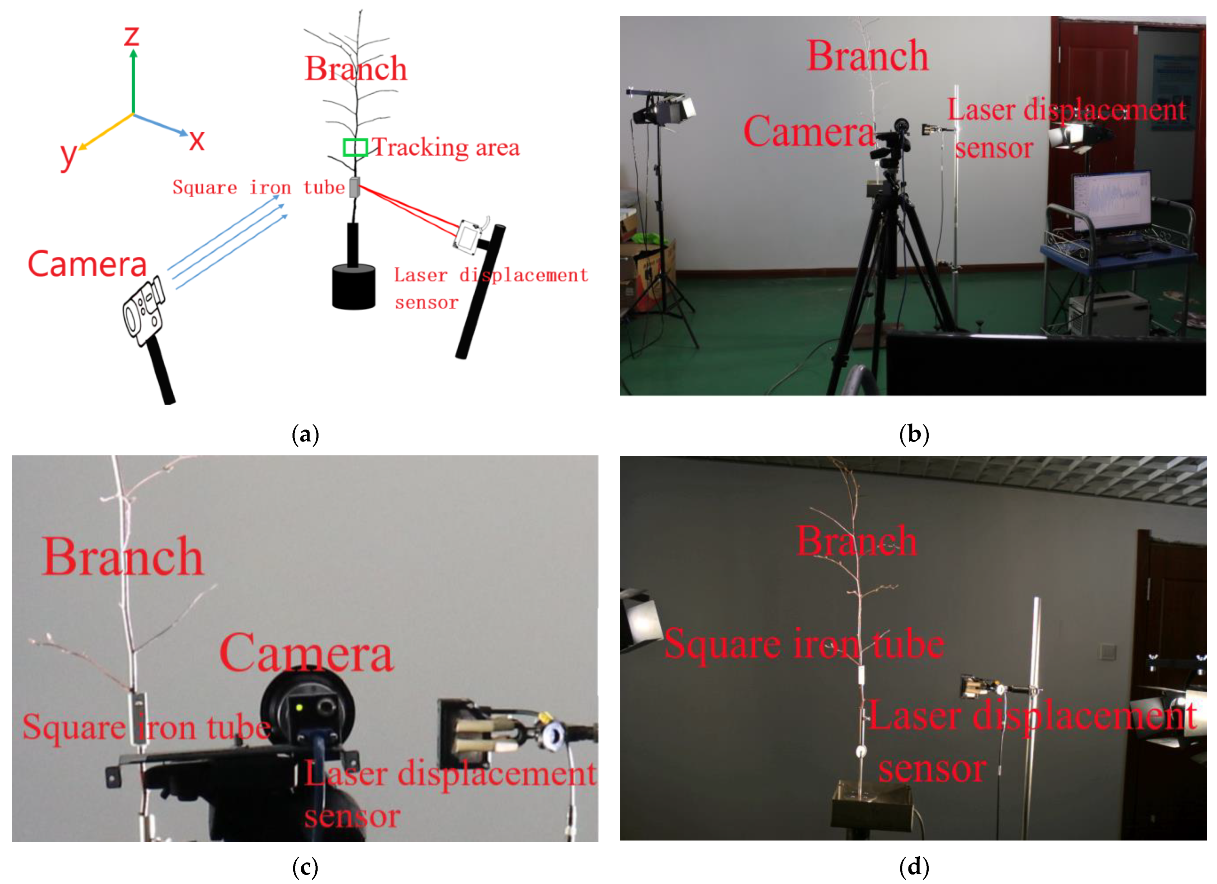
2.1.1. Data Collection of Branch Sway under Artificial Excitation Conditions

The experimental object was a tilt-growing branch, approximately 70 cm in length, taken from the middle part of a healthy Betula platyphylla Sukaczev crown on the campus of Northeast Forestry University, which was used for no more than 5 h in the experiment. The thickest part of the branch is approximately 1 cm in diameter. The sway frequency of the branch is related to the base diameter of the tree, Young’s elastic modulus and wood density [44]. The physical parameters of the cut branch do not change, so the sway frequency of the cut branch does not change. The schematic diagram of the data acquisition system is shown in Figure 1a, where a laser displacement sensor (CMOSIL-300, Keyence, Osaka, Japan) was used to measure the displacement in the x-axis direction of the branch. The linearity of the laser displacement sensor is ±0.25% f.s., the measurement range is 160–440 mm, and the sampling frequency is 200 Hz. In the experiment, in order to conveniently measure the horizontal displacement of the branch, the branch was fixed vertically. Since the branch is thin, the multi-DOF sway of the branch after being pulled may cause the laser emitted by the laser displacement sensor to deviate from the branch, resulting in the loss of measurement data. To solve this problem, a square iron tube was attached to the branch to increase the region for laser irradiation. This ensured that the laser emitted by the laser displacement sensor remained on the iron tube while the branch was swaying, thereby guaranteeing that the collected data were not lost. The camera (MER-230-168U3M/C, Daheng (group) Co., Ltd., Beijing, China) was aimed at the branch and perpendicular to the laser emission direction of the laser displacement sensor. The resolution of the camera was 1920 (H) × 1200 (V) and the focal length was 35 mm. The sampling frequency of the video was set to 40 Hz considering the video resolution and tracking effect. The placement of data acquisition equipment is shown in Figure 1b. An enlarged picture of the placement of the branch, laser displacement sensor and camera is shown in Figure 1c. The picture taken by the camera is shown in Figure 1d.
In the experiment, three groups of artificial excitation experiments were carried out to avoid the contingency of the experiment. The branch was pulled in the x-axis direction to make it sway. In order to avoid the influence of the square iron pipe on the tracking of the branch in the video, the tracking region selected in the video did not coincide with the monitoring region of the laser displacement sensor, as shown in Figure 1a. While pulling the branch, the camera was turned on for shooting, while the laser displacement sensor started data collection, and the sampling time was set to 18 s.

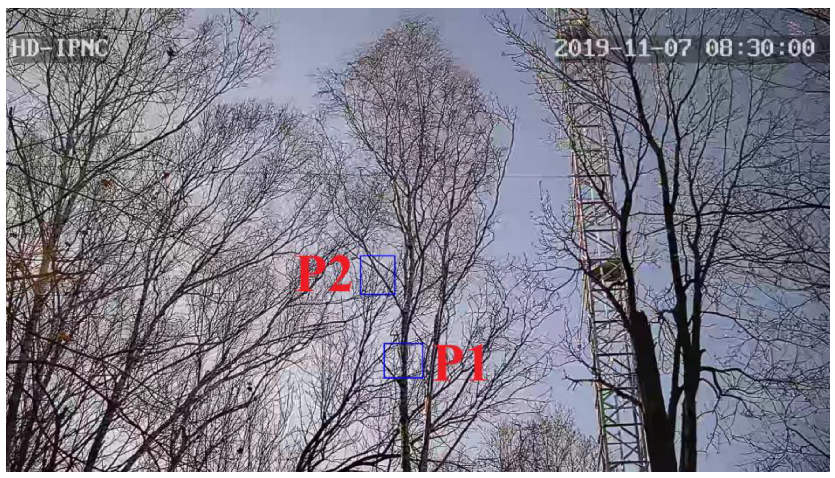
2.1.2. Data of Tree Sway under Environmental Excitation Conditions

A natural-growing Betula platyphylla Sukaczev tree with a height of 23.2 m and a diameter at breast height (DBH) of 27.4 cm was selected as the experiment object, which was located in the Maoershan Forest Ecosystem National Field Scientific Observation and Research Station (127°39′50″ E, 45°24′32″ N). Xin et al. [45] conducted a pulling test on the tree and analyzed the collected acceleration response data using the Fourier transform. The peak frequencies of the two acceleration components under free vibration of the tree were found to be 0.28 Hz and 0.26 Hz, respectively. Wang et al. [1] selected 10 segments of 30 min videos of the tree during a period of strong winds in autumn. They tracked two positions of the tree in the videos and measured the fundamental sway frequency of the tree based on the tracking results. The power spectral density (PSD) of the frequency measurements at the two positions is shown in Figure 2. The peak frequencies were 0.27 Hz and 0.26 Hz, respectively.
In this experiment, we selected two positions, P1 and P2, on the primary and secondary branches for tracking and frequency measurement based on the 10 videos used by Wang et al. (2022) [1]. The tracking regions are shown in Figure 3. The video frame rate was 16 Hz, and in order to compare the results with those of Wang et al. (2022) [1], the sampling frequency was set to 4 Hz, the same as in Wang et al. (2022) [1].

2.2. Tracking Methods

2.2.1. Online Boosting Algorithm

The online Boosting algorithm regards the tracking problem as the classification problem of target and background [32]. In the process of tracking, the online Boosting algorithm is used to adaptively select discriminative features, and the classifier is adaptively changed for tracking according to the change of the target. The online Boosting tracker is composed of N-weighted selectors to form a strong classifier, and the strong classifier is used to detect the target position in the next frame. There is a feature pool for each selector (each selector consists of M weak classifiers, and each weak classifier corresponds to a feature). When a new video frame arrives, each selector updates all the weak classifiers, selects the weak classifier with the smallest error, and linearly accumulates them to form the strong classifier.

2.2.2. Online MIL Algorithm

Babenko [33] proposed a tracking algorithm based on online Multiple Instance Learning (MIL), the key of which is to obtain a strong classifier. During the computation, positive and negative sample bags are generated separately, with the positive sample bag containing at least one positive sample and the negative sample bag not containing any positive samples. Then, the probabilities of each sample in the positive bag or negative bag were calculated according to the distribution of each sample. By maximizing the value of a logarithmic likelihood function through learning, a weak classifier is obtained. This process is repeated several times to obtain multiple weak classifiers, which are then combined to form a strong classifier. When a new frame arrives, the obtained strong classifier is used to classify the newly collected samples. The position of the sample with the highest classification result is regarded as the position to be tracked.

2.2.3. TLD Algorithm

The Tracking–Learning–Detection (TLD) algorithm, proposed by Kalal, is a robust object-tracking algorithm [34]. This algorithm decomposes the tracking task into three modules: tracking, learning, and detection. Firstly, the video was input into the tracking and detection module working in parallel to achieve tracking and detection. Secondly, the learning module evaluated the samples of the detection module according to the results of the tracking module, and generated training samples according to the evaluation results to update the model of the detection module and the “key feature points” of the tracking module, which were fed back into the parallel detection module and the tracking module in time. Finally, through the information integration of the integrator module, the real-time status of the target was obtained to achieve continuous tracking.

2.2.4. MOSSE Algorithm

Bolme et al. [23] introduced the principle of correlation filtering into the field of target tracking and proposed the Minimum Output Sum of Squared Error Filter tracker (MOSSE). The algorithm converts the convolution operation between the image template and the target image in the spatial domain into an equivalent multiplication operation in the frequency domain. This process significantly reduces the computation time of the algorithm and improves tracking efficiency. In the process of target tracking, feature extraction is performed on the first frame of the input video, the correlation filter is initialized, and the initial sample model of the target region is formed. Then, the region that best matches the sample model is searched frame by frame to achieve target tracking. Finally, the region with the highest correlation response is taken as the tracking result and input into the correlation filter to update the sample model.

2.2.5. KCF Algorithm

Henriques et al. [37] proposed the Kernel Correlation Filter (KCF) to improve the ability of the tracker to distinguish the target from the environmental background by applying a linear kernel to the extracted target features. The algorithm constructs a large number of samples in the target region by cyclically shifting the initial frame through the cyclic matrix, solving the problem of insufficient training samples in the target tracking process. At the same time, the property of cyclic matrix diagonalization greatly simplifies the calculation. The Histogram of Oriented Gradient (HOG) features are extracted from the samples to obtain positive and negative samples and distinguish the target from the background. Ridge regression is used to train the classifier and detect the object. The region with the highest response value is where the target is located, and the new target region is used as the training sample for the next frame to update the classifier.

2.2.6. CSR-DCF Algorithm

Lukežič proposed the CSR-DCF (Channel and Spatial Reliability–Discriminative Correlation Filter) tracker [39], which uses spatial segmentation and channel response values to evaluate the reliability of the spatial and channel, and conducts targeted tracking. This algorithm requires the input of the target position, region, filter, color histogram and channel confidence of the initial frame. When a new frame arrives, the target position is dot-multiplied using the filter and the picture block feature of the new frame and weighted by the channel confidence to obtain the position with the largest response as the target position of the new frame. Then, the target position in the new frame is used to estimate the current region, and the histograms of the foreground and background are obtained and updated, the spatial confidence map is calculated, the filter is estimated from it and the channel confidence is calculated. Finally, the filter weights and channel confidence are updated.

2.3. Frequency Measurement

The laser displacement sensor was used to measure the sway frequency of the branch, and the displacement data in the x-axis direction of the measured branch were directly analyzed using Fast Fourier Transform (FFT) to identify the sway frequency of the branch.
The method of measuring frequency by video adopts the method of measuring tree sway frequency proposed by Wang et al. [1], which is to perform FFT on the instantaneous average speed in the horizontal (x-direction) of the video to obtain the sway frequency of the tree. The details are as follows: in the tree sway tracking process, the point in the upper left corner of the rectangular tracking window is selected as the feature point to obtain the feature point coordinates of the tracking window. Using the change in the horizontal coordinates of the feature point in the video frames during this process, the average speed in the x-axis direction between two video frames is calculated as shown in Equation (1):
v x = X i X i 1 Δ t ,
v x is the average velocity, which can be considered as the instantaneous velocity between two frames of the video; X i is the coordinate value of the feature point along the x-axis on frame i ; X i 1 is the coordinate value of the feature point in the x-direction on frame i 1 ; and Δ t is the time interval between two adjacent frames. The power spectral density diagram of the tree is obtained by using the time series data of v x for FFT, and the peak frequency is the tree sway frequency.

2.4. Evaluation Metrics for Tracking Algorithms

The applicability of six target tracking algorithms for tree sway tracking and frequency measurement was evaluated from three aspects: tracking speed, tracking situation and accuracy of sway frequency measurement.
The tracking speed of the algorithm was evaluated by comparing the tracking time of six tracking algorithms for the same length of video. The tracking situation was evaluated by observing the position of the tracking window in the initial and final frames, as well as the changes in the feature points during the tracking process. This evaluation was performed using qualitative judgment to determine if the tracking method was suitable for tree sway tracking. The accuracy of measuring the sway frequency of the branch under artificial excitation conditions was evaluated by comparing the results obtained from the video with those obtained from the laser displacement sensor. The accuracy of measuring the tree sway frequency under environmental excitation conditions was evaluated by comparing the results obtained from different tracking algorithms with those obtained from Wang et al. [1] and Xin et al. [45].

3. Results

3.1. Experimental Results of Branch Sway under Artificial Excitation Conditions

In the experiment, 18 s of data were collected. However, during the experiment, the experimenter was filmed in the video, which affected the tracking effect; therefore, the data from the first 3 s were used, and the data of the remaining 15 s collected by both the laser displacement sensor and the video were selected for analysis.

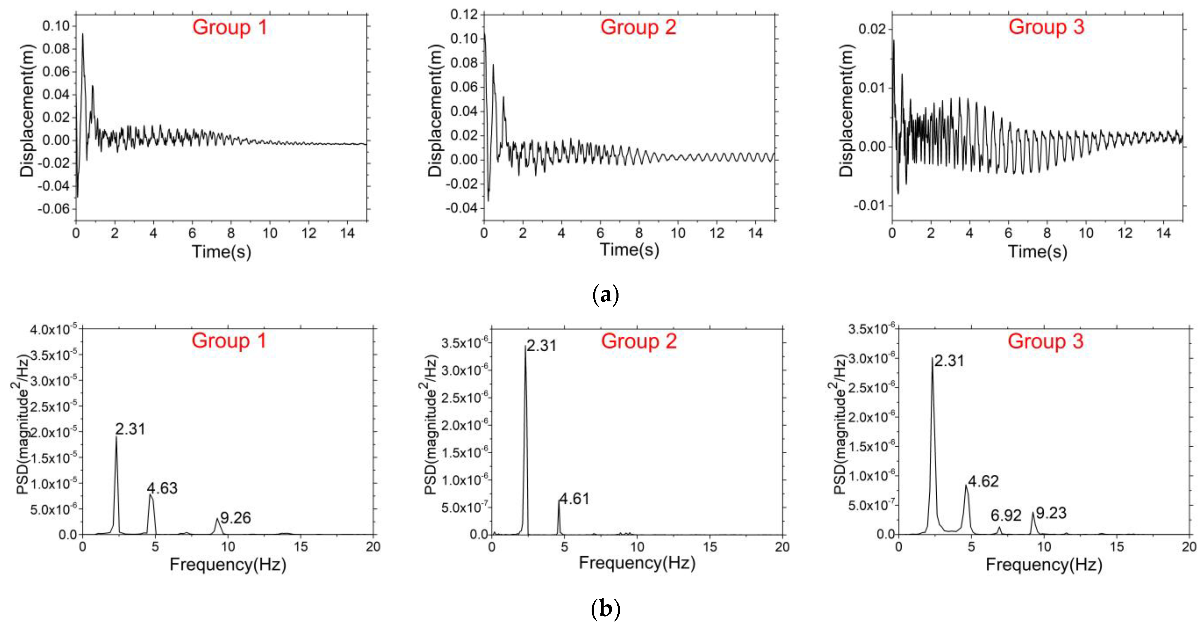
3.1.1. The Measurement Results of the Laser Displacement Sensor

Under artificial excitation conditions, the 15 s displacement of the branch was measured by the laser displacement sensor, as shown in Figure 4a. As can be seen from Figure 4a, the points on the vertical axis at 0 represent the position of the branch when it was stationary. After artificial excitation, in the experiments of groups 1 and 2, the branch swayed significantly in the x direction, followed by a gradual decrease in amplitude, indicating a signal decay movement. In the experiment of group 3, the branch in the x-direction swayed initially, after which the amplitude decreased, increased, and then gradually decreased again. The signal was not gradually decaying, which was due to the branch swaying with multiple degrees of freedom after being excited, and what was measured was only the displacement in the x direction. Meanwhile, the initial sway of the branch in the x direction did not oscillate around the position at rest (0 point), which was related to the multiple degrees of freedom of the branch; as the energy dissipated, the movement in the x direction gradually became the dominant motion, oscillated around the position at rest, and the displacement in the x-direction showed a relatively stable signal free decay characteristic. Taking the signal with obvious free decay characteristics, FFT was used for spectrum analysis. Because the sampling frequency of the video was 40 Hz, according to the sampling theorem, the frequency range of the power spectrum obtained by the laser displacement sensor was limited to 20 Hz for easy comparison with the video measurement results. The obtained PSD is shown in Figure 4b.
As can be seen from Figure 4b, the first three order frequencies measured in the experiment of group 1 were 2.31 Hz, 4.63 Hz and 9.26 Hz, respectively; the first three order frequencies measured in the experiment of group 2 were 2.32 Hz, 4.62 Hz and 6.95 Hz, respectively; the first four order frequencies measured in the experiment of group 3 were 2.31 Hz, 4.62 Hz, 6.92 Hz and 9.23 Hz, respectively. The first two order frequencies measured in the three groups of experiments were close. Among them, the first-order frequency was the basic sway frequency of the branch. In addition, the higher-order frequencies measured in the three groups of experiments were not consistent, which may be because the sway of the branch was a multi-degree freedom movement, and the frequencies in the experiment were only based on the displacement data in the x direction for FFT spectrum analysis.

3.1.2. Tracking Time

The tracking time for the 15 s video of the three groups of experiments based on six tracking methods is shown in Table 1. The tracking time from long to short was TLD, MIL, Boosting, CSR-DCF, KCF and MOSSE, with an average time of 150.05 s, 63.82 s, 51.07 s, 36.14 s, 21.05 s and 9.55 s, respectively. Among them, the fastest was the MOSSE algorithm, and the slowest was the TLD algorithm.

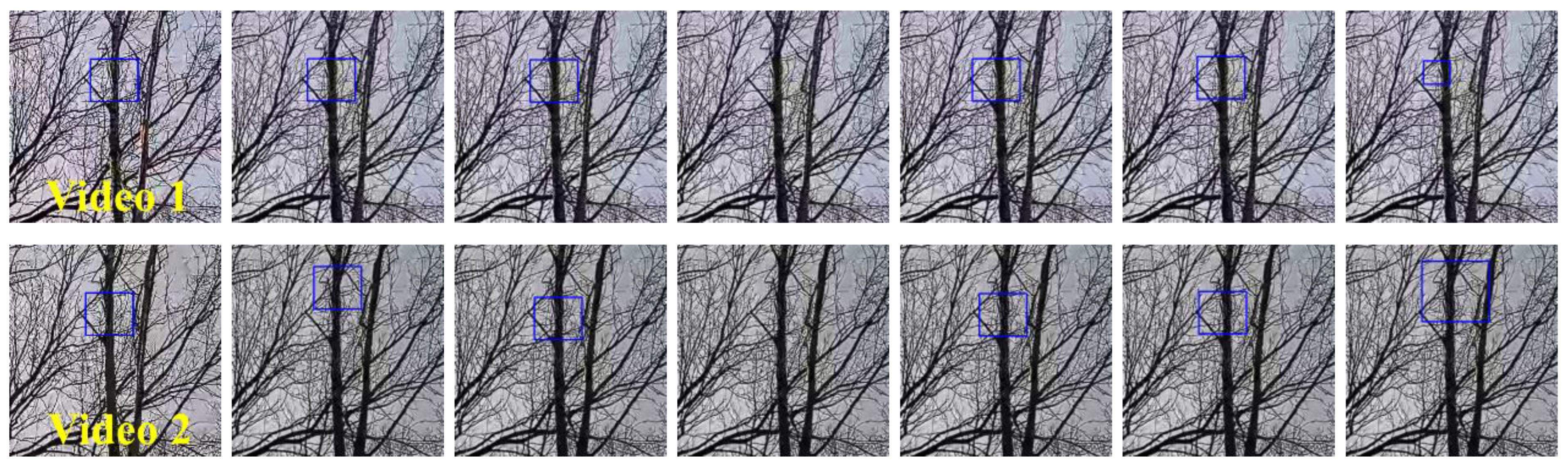
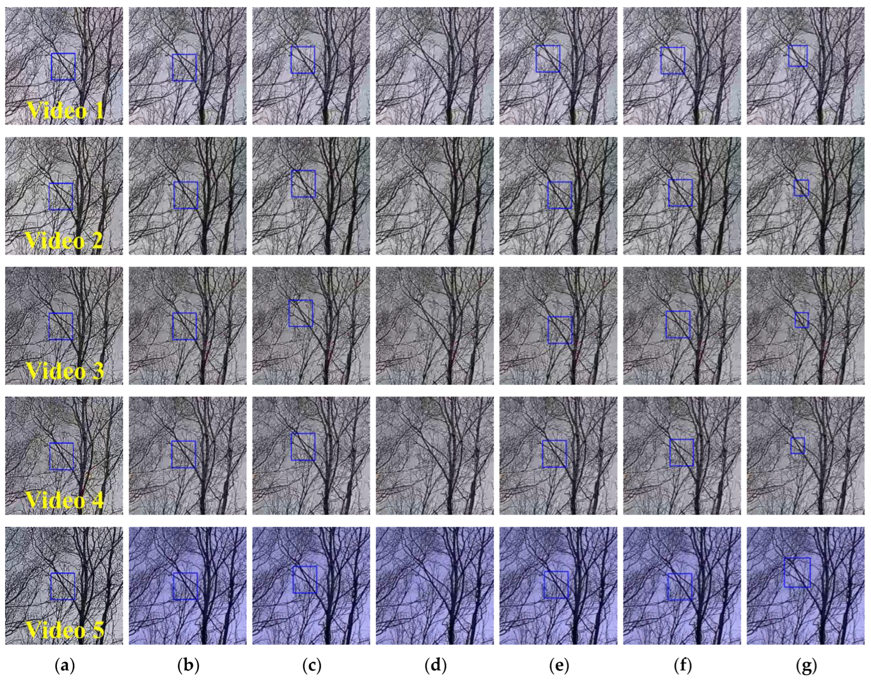
3.1.3. Tracking Situation

The positions of the tracking windows based on the six tracking methods in the initial frame and the last frame of the three groups of experiments are shown in Figure 5. As can be seen from the figure, at the end of the 15 s tracking, the TLD algorithm failed in the experiments of groups 1 and 3, and the tracking window changed in scale; the CSR-DCF was successful in tracking, and the tracking window changed in scale; the Boosting, MIL, MOSSE and KCF were successful in tracking, and the scale of the tracking window did not change.
The coordinate changes in the feature points along the X-axis in the video obtained by using the six tracking methods to track the branch sway under the artificial excitation conditions are shown in Figure 6. Among them, the tracking results based on Boosting, MIL and MOSSE can see obvious fluctuation signals, reflecting the sway motion of the branch. For TLD, the coordinate values changed significantly, after which the tracking window deviated from the target, the method failed in tracking and it could not reflect the sway motion of the branch. For KCF, although the tracking window did not deviate from the target, the tracking trajectory underwent rapid and dense repeated fluctuations, which could not reflect the sway motion of the branch. For CSR-DCF, although the fluctuation of the signal can be seen, because the tracking window changed in scale, the fluctuation was not consistent with the real sway motion of the branch.

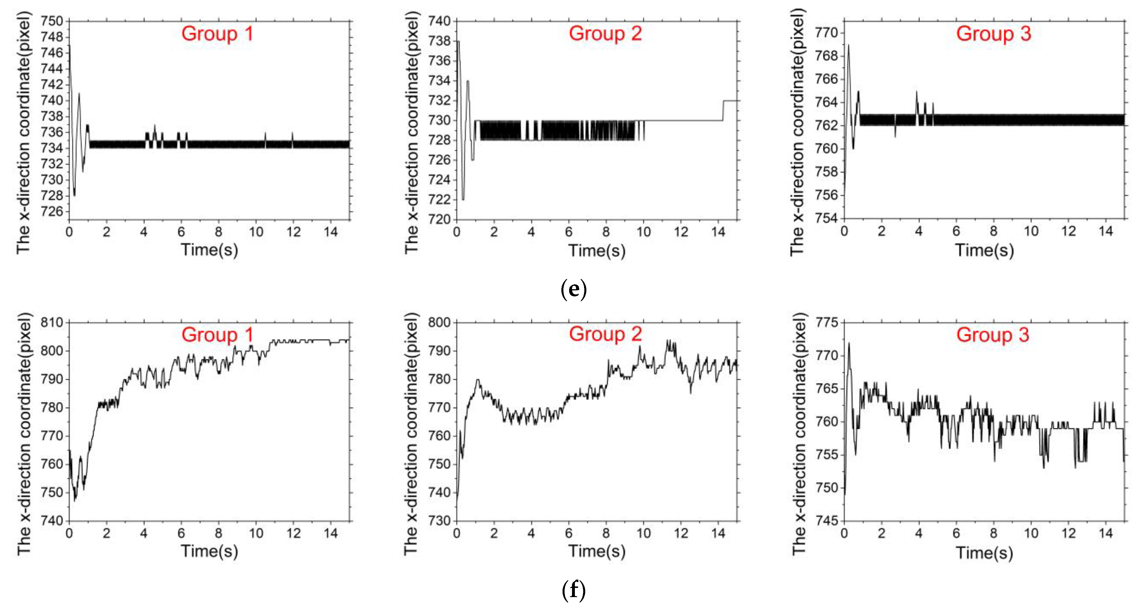
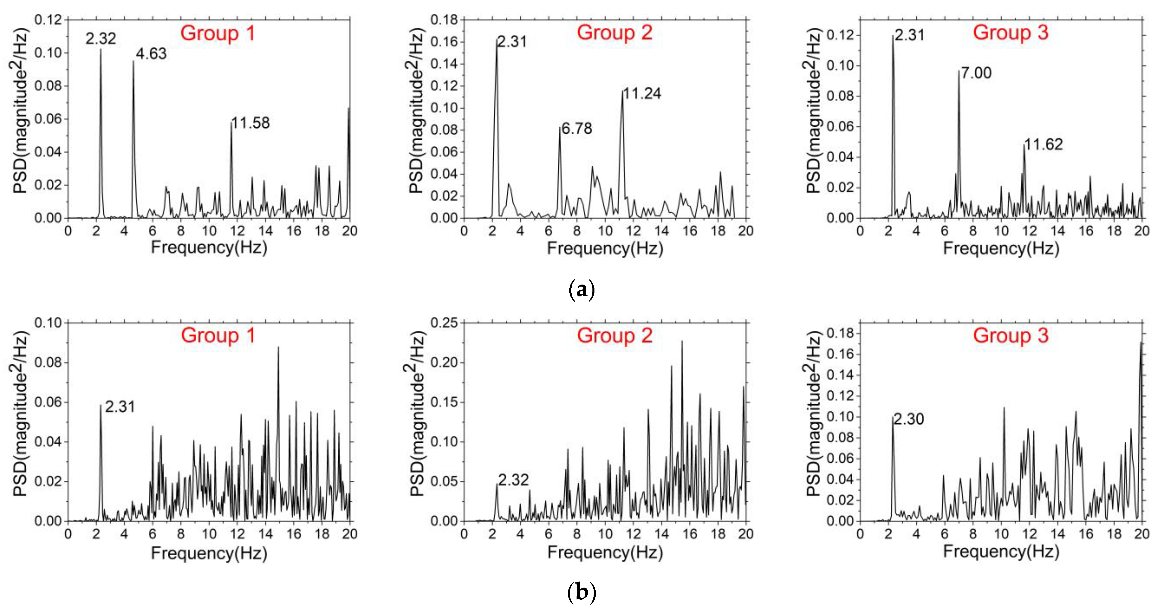
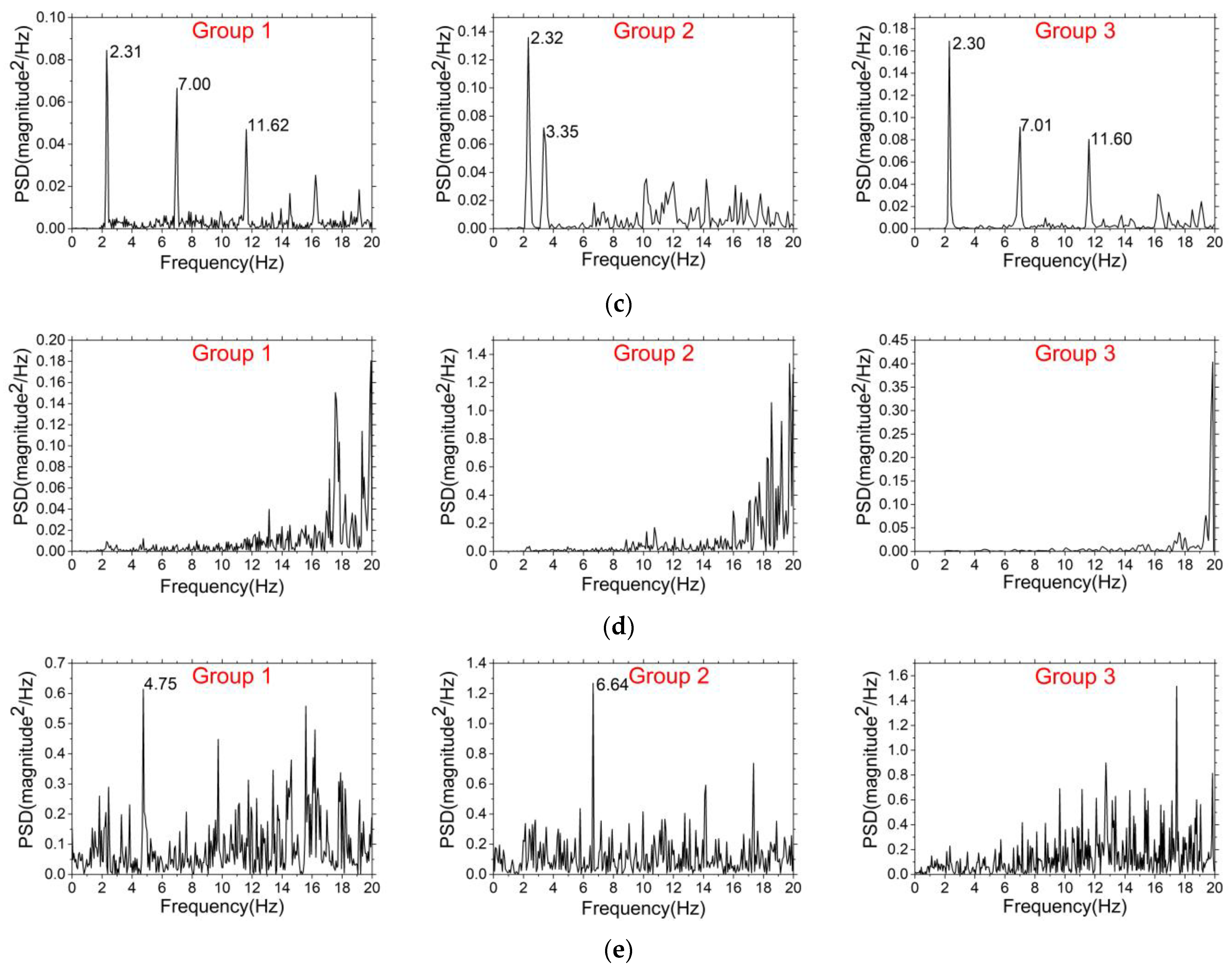
3.1.4. Frequency Measurement Results Based on Video Method

The TLD algorithm was obviously inappropriate for frequency measurement since target loss occurred in the branch sway tracking. For the coordinate data of feature points in the X-axis direction obtained by Boosting, MIL, KCF, MOSSE and CSR-DCF algorithms in the video with obvious signal fluctuations, the instantaneous velocity was calculated according to Equation (1), and the obtained velocity data were analyzed by FFT, and the results are shown in Figure 7.
As can be seen from Figure 7, KCF and CSR-DCF algorithms could not accurately measure the sway frequency of the branch, which was caused by the fact that these two algorithms could not reflect the true motion of the branch. The measurement results of the video and the laser displacement sensor were compared, and the significant peaks measured by various methods are shown in Table 2. Among them, the first-order frequencies measured by the three tracking methods of Boosting, MIL and MOSSE were similar. The frequencies were basically consistent with the basic sway frequencies of the branch measured by the laser displacement sensor. However, the three methods were not consistent with the results measured by the laser displacement sensor in high-order frequency measurement. Only the second-order frequency measured by the Boosting algorithm in the first group of experiments was consistent with the measurement result of the laser displacement sensor. The measurement results of the other groups of experiments were different from those of the laser displacement sensor in the measurement of frequencies above the second order, which may have been caused by the drift and different measurement positions in the tracking.

3.2. Experimental Results of Tree Sway under Environmental Excitation Conditions

3.2.1. Tracking Time

The average tracking time of the 10 30-min videos at P1 and P2 based on six tracking methods is shown in Table 3. As can be seen from Table 3, the tracking time from long to short was TLD, MIL, Boosting, CSR-DCF, KCF and MOSSE, with a total average time of 2414.52 s, 1075.16 s, 738.21 s, 707.48 s, 532.19 s and 459.22 s, respectively. Among them, the fastest was MOSSE, and the slowest was TLD.

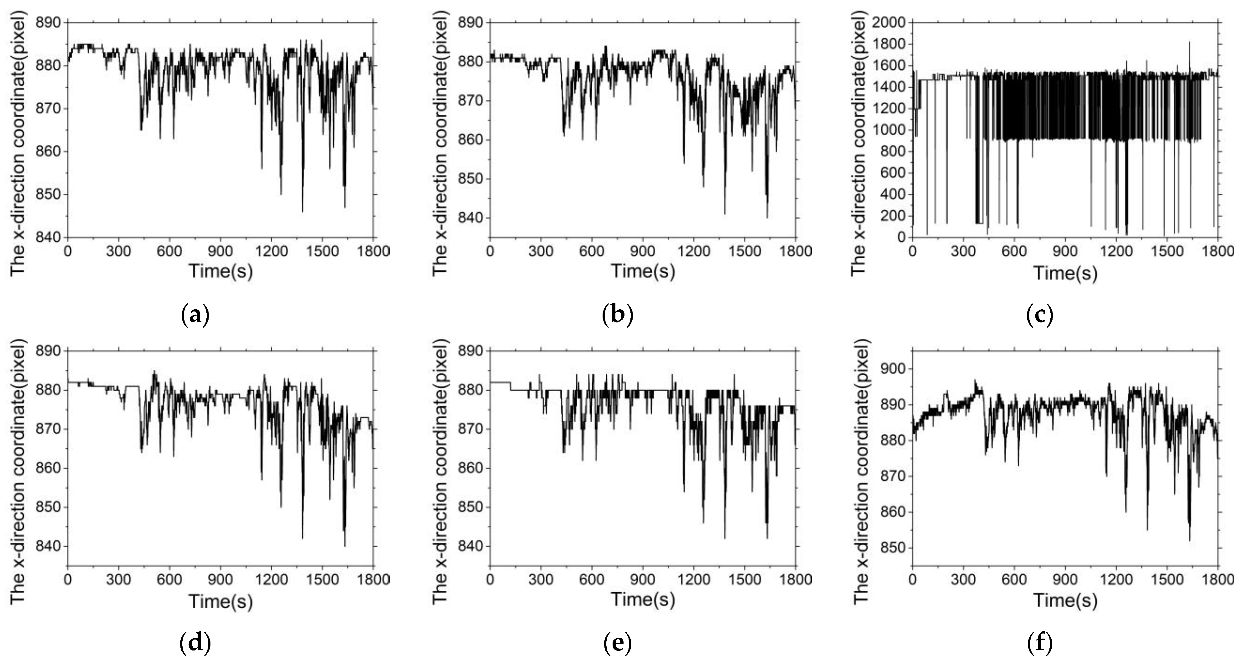
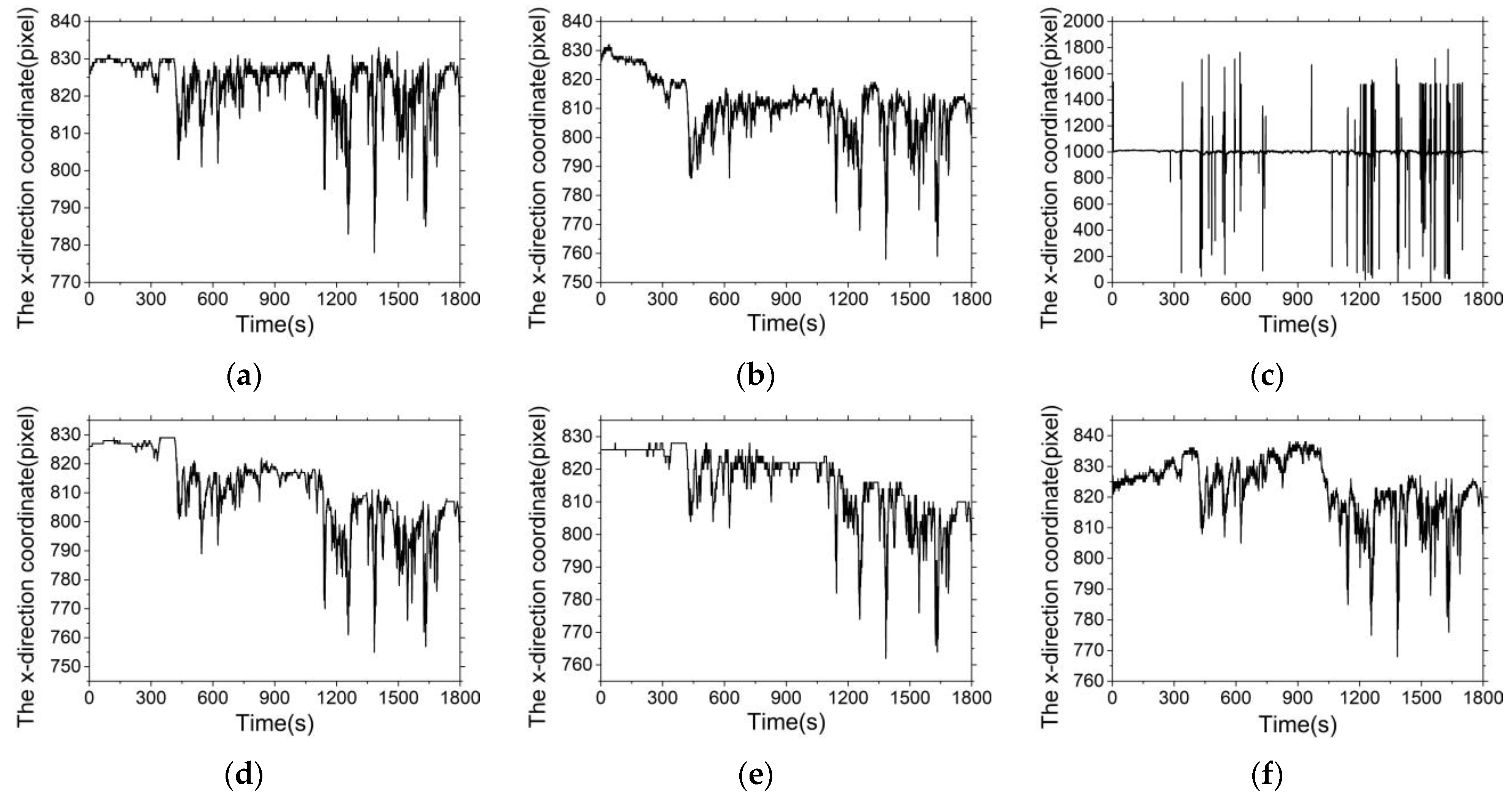
3.2.2. Tracking Situation

Based on six tracking methods for tracking P1 and P2, the positions of the tracking window in the initial frame and the last frame of the first five videos are shown in Figure 8 and Figure 9. As can be seen from Figure 8 and Figure 9, the TLD algorithm failed; the CSR-DCF algorithm succeeded, with the tracking window changed in scale; the Boosting, MIL, MOSSE and KCF algorithms succeeded, with no changes in scale of the tracking window.
Based on six tracking methods to track P1 and P2, the changes in the target feature points along the x-axis in the first video obtained are shown in Figure 10 and Figure 11. From the figures, it can be seen that the tracking results of Boosting, MIL, MOSSE, KCF and CSR-DCF showed obvious fluctuation signals, reflecting the tree sway motion. The tracking result of TLD showed a significant tracking offset and could not reflect the tree sway motion. It should be noted that although the tracking result of CSR-DCF showed an obvious fluctuation signal, the fluctuation of the signal could not completely coincide with the tree sway motion due to the change in the tracking window scale.

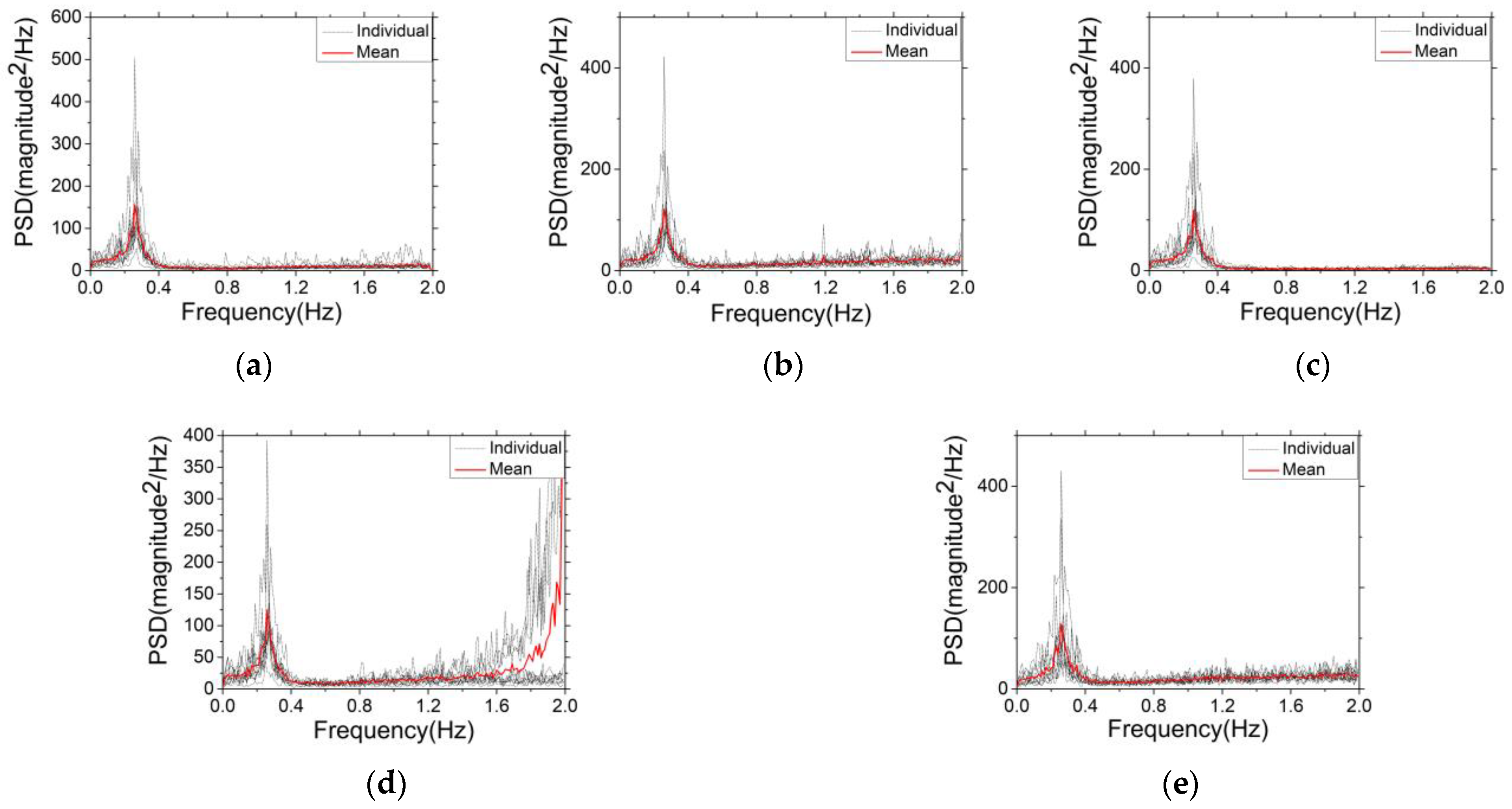
3.2.3. Frequency Measurement Results Based on Video Method

The TLD algorithm was not suitable for frequency measurement because it suffered from target tracking loss during tree sway tracking. For the x-axis coordinate data of feature points in P1 and P2 obtained from the other five tracking methods, the instantaneous velocity was calculated using Equation (1), and FFT spectrum analysis was performed. The PSD was averaged over a bandwidth of 0.01 Hz to enhance the statistical stability of the estimates. The resulting PSDs are shown in Figure 12 and Figure 13.
As can be seen from Figure 12 and Figure 13, the PSD obtained by the five tracking methods at positions P1 and P2 had a recognizable peak between 0.2 Hz and 0.4 Hz, both at 0.26 Hz, which was the sway frequency of the tree. The results were consistent with the sway frequency measured by Wang et al. [1] and Xin et al. [45]. In addition, the sway frequencies of the tree measured at P1 and P2 were equal, which was consistent with the results of Wang et al. [1] and Baker [16] that the sway frequencies measured at different positions on the same tree were close or the same.

4. Discussion

Video-based methods are widely used by researchers in the study of agriculture and forestry due to their advantages of convenient data collection, non-contact, and high-cost performance. However, research on tree swaying monitoring and frequency measurement based on video methods is still rare, and the key to video methods is the selection of tracking methods. In this study, we explored the effectiveness of six representative tracking methods in tracking tree sway and the accuracy of measuring tree sway frequency.
The accuracy of measuring the sway frequency of trees depends on whether the tracking results of the tracking method used can accurately reflect the sway of the trees. The TLD algorithm is not suitable for measuring the sway frequency of trees due to the failure of tracking, as it cannot reflect the actual movement of trees. The Boosting, MIL and MOSSE tracking methods can accurately measure the sway frequency of trees under both artificial and environmental conditions. This is because these three tracking methods are scale-invariant, and the distance from the base of the tree to the camera does not change during the tree sway. The motion of the tracking region relative to the camera can be simply understood as planar motion; based on this, the points on the scale-invariant tracking frame can accurately reflect the sway of the tree in the x-axis direction.
Based on the KCF and CSR-DCF algorithms, the sway frequency of the branch under artificial excitation conditions cannot be measured; however, the sway frequency of the tree under environmental excitation conditions can be measured, which may be caused by the drift and scale change in the tracking window itself. The rapid dense small-scale drift motion based on the KCF algorithm and the scale change in the tracking window based on the CSR-DCF algorithm will cause a difference between the tracking trajectory and the actual sway trajectory of the tree. Under artificial excitation conditions, because the sway amplitude of the branch is small, the value of this difference is not much different from the sway amplitude, resulting in the motion of the tracked feature points not reflecting the actual sway of the branch, so the sway frequency of the branch cannot be accurately measured. However, under environmental excitation conditions, the tree to be measured sways greatly in the strong wind, the value of the difference caused by the above two tracking methods is far less than the actual sway amplitude of the tree, and the change in the feature points can still accurately reflect the actual sway of the tree, so the frequency of the tree can be accurately measured.
This study explored the effect of six different tracking algorithms on tree sway tracking and frequency measurement, but there are still some limitations in this study, which are worth further exploration in the future. In the selection of research objects, only a leafless birch branch and a leafless deciduous tree were selected, and more research objects (multiple leafless branches and multiple leafless trees), branches with leaves, full-leaf trees and other tree species were not tested. Chau et al. used a novel multi-beam flash light detection and ranging (LiDAR) sensor to measure the frequencies of one Liquidambar formosana, three Araucaria heterophylla trees, one Sterculia lanceolata, one Celtis sinensis, one Tabebuia chrysantha and one Cinnamomum camphora, and found that broadleaved trees might exhibit vibration in a wide frequency band, whereas the coniferous trees could follow a distinct dominant frequency [20]. In addition, in the discussion of tracking situation, only qualitative analysis was carried out, without quantitative comparison. In future research, quantitative research methods will be further used to compare different object tracking methods in terms of sway tracking and frequency measurement of multi-object, multi-species and full-leaf trees.

5. Conclusions

In this study, the feasibility and effectiveness of six tracking algorithms for measuring the sway frequencies of a Betula platyphylla Sukaczev branch taken from the campus of Northeast Forestry University and a Betula platyphylla Sukaczev tree in the Maoershan Forest Ecosystem National Field Scientific Observation and Research Station were verified and compared under two conditions of artificial and environmental excitation.
  • The speed of tree sway tracking of the six tracking methods from fast to slow was MOSSE, KCF, CSR-DCF, Boosting, MIL and TLD.
  • The TLD algorithm was not suitable for tree sway tracking, and could not be used to measure the tree sway frequency. The tracking window of Boosting, MIL, MOSSE and KCF did not change in scale, and the tracking window of CSR-DCF changed in scale; these five algorithms did not lose the tracking object and can be used for tree sway tracking.
  • In the measurement of the branch sway frequency under artificial excitation conditions, the Boosting, MIL and MOSSE methods can accurately measure the branch sway frequency to solve the problem of the contact sensor being difficult to install on thin branches, and its own weight may affect the measurement results.
  • Based on Boosting, MIL, MOSSE, KCF and CSR-DCF methods, the sway frequency of trees can be accurately measured under environmental excitation conditions.

Author Contributions

X.Y. and A.W. designed the experiment. X.Y. carried out the experiments. X.Y. and P.P. analyzed the data and wrote the original manuscript with the help and critique of A.W. All authors have read and agreed to the published version of the manuscript.

Funding

This research was funded by the Natural Science Foundation of Heilongjiang Province of China, grant number LH2021F050; the 2022 Special Foundation Project of Fundamental Scientific Research Professional Expenses for Undergraduate Universities in Heilongjiang Province, grant number 2022-KYYWF-0474.

Institutional Review Board Statement

Not applicable.

Informed Consent Statement

Not applicable.

Data Availability Statement

The research data are available upon request from the corresponding author.

Conflicts of Interest

The authors declare no conflict of interest.

References

  1. Wang, A.; Yang, X.; Xin, D. The Tracking and Frequency Measurement of the Sway of Leafless Deciduous Trees by Adaptive Tracking Window Based on MOSSE. Forests 2022, 13, 81. [Google Scholar] [CrossRef]
  2. Yang, X.; Wang, A.; Jiang, H. Intelligent Measurement of Frontal Area of Leaves in Wind Tunnel Based on Improved U-Net. Electronics 2022, 11, 2730. [Google Scholar] [CrossRef]
  3. Bayat, M.; Ghorbanpour, M.; Zare, R.; Jaafari, A.; Pham, B.T. Application of Artificial Neural Networks for Predicting Tree Survival and Mortality in the Hyrcanian forest of Iran. Comput. Electron. Agric. 2019, 164, 104929. [Google Scholar] [CrossRef]
  4. Bayat, M.; Noi, P.T.; Zare, R.; Bui, D.T. A Semi-Empirical Approach Based on Genetic Programming for the Study of Biophysical Controls on Diameter-Growth of Fagus Orientalis in Northern Iran. Remote Sens. 2019, 11, 1680. [Google Scholar] [CrossRef]
  5. Bayat, M.; Bettinger, P.; Heidari, S.; Hamidi, S.K.; Jaafari, A. A Combination of Biotic and Abiotic Factors and Diversity Determine Productivity in Natural Deciduous Forests. Forests 2021, 12, 1450. [Google Scholar] [CrossRef]
  6. Bunce, A.; Volin, J.C.; Miller, D.R.; Parent, J.; Rudnicki, M. Determinants of tree sway frequency in temperate deciduous forests of the Northeast United States. Agric. For. Meteorol. 2019, 266–267, 87–96. [Google Scholar] [CrossRef]
  7. Lee, L.S.H.; Jim, C.Y. Applying precision triaxial accelerometer to monitor branch sway of an urban tree in a tropical cyclone. Landsc. Urban Plan. 2018, 178, 170–182. [Google Scholar] [CrossRef]
  8. Moore, J.R.; Maguire, D.A. Simulating the dynamic behavior of Douglas-fir trees under applied loads by the finite element method. Tree Physiol. 2008, 28, 75–83. [Google Scholar] [CrossRef]
  9. Spatz, H.C.; Brüchert, F.; Pfisterer, J. Multiple resonance damping or how do trees escape dangerously large oscillations? Am. J. Bot. 2007, 94, 1603–1611. [Google Scholar] [CrossRef]
  10. Kane, B.; Clouston, P. Tree pulling tests of large shade trees in the genus Acer. Arboric. Urban For. 2008, 34, 101–109. [Google Scholar] [CrossRef]
  11. Der Loughian, C.; Tadrist, L.; Allain, J.M.; Diener, J.; Moulia, B.; De Langre, E. Measuring local and global vibration modes in model plants. Comptes Rendus Mécanique 2014, 342, 1–7. [Google Scholar] [CrossRef]
  12. Li, Z.; Zhao, D.; Zhong, M. Measurement and finite element analysis of the dynamic characteristics of trees. J. Vib. Shock 2022, 41, 271–280. [Google Scholar]
  13. Van Emmerik, T.; Steele-Dunne, S.; Hut, R.; Gentine, P.; Guerin, M.; Oliveira, R.S.; Wagner, J.; Selker, J.; Van De Giesen, N. Measuring Tree Properties and Responses Using Low-Cost Accelerometers. Sensors 2017, 17, 1098. [Google Scholar] [CrossRef] [PubMed]
  14. Koizumi, A.; Shimizu, M.; Sasaki, Y.; Hirai, T. In situ drag coefficient measurements for rooftop trees. J. Wood Sci. 2016, 62, 363–369. [Google Scholar] [CrossRef]
  15. James, K.R.; Kane, B. Precision digital instruments to measure dynamic wind loads on trees during storms. Agric. For. Meteorol. 2008, 148, 1055–1061. [Google Scholar] [CrossRef]
  16. Baker, C.J. Measurements of the natural frequencies of trees. J. Exp. Bot. 1997, 48, 1125–1132. [Google Scholar] [CrossRef]
  17. Hassinen, A.; Lemettinen, M.; Peltola, H.; Kellomäki, S.; Gardiner, B. A prism-based system for monitoring the swaying of trees under wind loading. Agric. For. Meteorol. 1998, 90, 187–194. [Google Scholar] [CrossRef]
  18. Barbacci, A.; Diener, J.; Hémon, P.; Adam, B.; Donès, N.; Reveret, L.; Moulia, B. A robust videogrametric method for the velocimetry of wind-induced motion in trees. Agric. For. Meteorol. 2014, 184, 220–229. [Google Scholar] [CrossRef]
  19. He, P.; Hu, S.; He, D. Trajectory Capture and Sway Frequency Analysis of Trees Based on Kinect. J. Syst. Simul. 2017, 29, 1411–1418. [Google Scholar]
  20. Chau, W.Y.; Loong, C.N.; Wang, Y.H.; Chiu, S.W.; Tan, T.J.; Wu, J.; Leung, M.L.; Tan, P.S.; Ooi, G.L. Understanding the dynamic properties of trees using the motions constructed from multi-beam flash light detection and ranging measurements. J. R. Soc. Interface 2022, 19, 20220319. [Google Scholar] [CrossRef]
  21. Bouguet, J.Y. Pyramidal Implementation of the Lucas Kanade Feature Tracker Description of the Algorithm; Intel Corporation Microprocessor Research Labs: Santa Clara, CA, USA, 2000. [Google Scholar]
  22. Xue, T.; Wu, J.; Zhang, Z.; Zhang, C.; Tenenbaum, J.B.; Freeman, W.T. Seeing Tree Structure from Vibration. Computer Vision. In Proceedings of the European Conference on Computer Vision (ECCV), Munich, Germany, 8–14 September 2018; pp. 762–779. [Google Scholar]
  23. Bolme, D.S.; Beveridge, J.R.; Draper, B.A.; Lui, Y.M. Visual object tracking using adaptive correlation filters. In Proceedings of the Twenty-Third IEEE Conference on Computer Vision and Pattern Recognition, San Francisco, CA, USA, 13–18 June 2010; pp. 13–18. [Google Scholar]
  24. Li, X.; Zha, Y.; Zhang, T.; Cui, Z.; Zuo, W.; Hou, Z.; Lu, H.; Wang, H. Survey of visual object tracking algorithms based on deep learning. J. Image Graph. 2019, 24, 2057–2080. [Google Scholar]
  25. Krizhevsky, A.; Sutskever, I.; Hinton, G.E. ImageNet classification with deep convolutional neural networks. Commun. ACM 2012, 60, 84–90. [Google Scholar] [CrossRef]
  26. Welch, G.; Bishop, G. An Introduction to the Kalman Filter; University of North Carolina at Chapel Hill: Chapel Hill, NC, USA, 2001. [Google Scholar]
  27. Nummiaro, K.; Koller-Meier, E.; Van, G.L. An adaptive color-based particle filter. Image Vis. Comput. 2003, 21, 99–110. [Google Scholar] [CrossRef]
  28. Comaniciu, D.; Ramesh, V.; Meer, P. Real-time tracking of non-rigid objects using mean shift. In Proceedings of the IEEE Conference on Computer Vision and Pattern Recognition. CVPR 2000 (Cat. No.PR00662), Hilton Head, SC, USA, 15 June 2000; pp. 142–149. [Google Scholar]
  29. Exner, D.; Bruns, E.; Kurz, D.; Grundhöfer, A.; Bimber, O. Fast and robust CAMShift tracking. In Proceedings of the 2010 IEEE Computer Society Conference on Computer Vision and Pattern Recognition-Workshops, San Francisco, CA, USA, 13–18 June 2010; pp. 9–16. [Google Scholar]
  30. Choi, J.Y.; Sung, K.S.; Yang, Y.K. Multiple Vehicles Detection and Tracking based on Scale-Invariant Feature Transform. In Proceedings of the 2007 IEEE Intelligent Transportation Systems Conference, Bellevue, WA, USA, 30 September–3 October 2007; pp. 528–533. [Google Scholar]
  31. Bay, H.; Tuytelaars, T.; Van, G.L. SURF: Speeded Up Robust Features. Lect. Notes Comput. Sci. 2016, 3951, 404–417. [Google Scholar]
  32. Grabner, H.; Grabner, M.; Bischof, H. Real-Time Tracking via On-line Boosting. In Proceedings of the British Machine Vision Conference, Edinburgh, UK, 4–7 September 2006. [Google Scholar]
  33. Babenko, B.; Yang, M.H.; Belongie, S. Visual tracking with online Multiple Instance Learning. In Proceedings of the 2009 IEEE Conference on Computer Vision and Pattern Recognition, Miami, FL, USA, 20–25 June 2009; pp. 983–990. [Google Scholar]
  34. Kalal, Z.; Mikolajczyk, K.; Matas, J. Tracking-Learning-Detection. IEEE Trans. Pattern Anal. Mach. Intell. 2012, 34, 1409–1422. [Google Scholar] [CrossRef]
  35. Henriques, J.F.; Caseiro, R.; Martins, P.; Batista, J. Exploiting the Circulant Structure of Tracking-by-Detection with Kernels. In Proceedings of the Computer Vision-ECCV 2012, Florence, Italy, 7–13 October 2012; pp. 702–715. [Google Scholar]
  36. Danelljan, M.; Häger, G.; Khan, F.S.; Felsberg, M. Accurate Scale Estimation for Robust Visual Tracking. In Proceedings of the British Machine Vision Conference, Nottingham, UK, 1–5 September 2014. [Google Scholar]
  37. Henriques, J.F.; Caseiro, R.; Martins, P.; Batista, J. High-Speed Tracking with Kernelized Correlation Filters. IEEE Trans. Pattern Anal. Mach. Intell. 2015, 37, 583–596. [Google Scholar] [CrossRef]
  38. Galoogahi, H.K.; Fagg, A.; Lucey, S. Learning Background-Aware Correlation Filters for Visual Tracking. In Proceedings of the 2017 IEEE International Conference on Computer Vision (ICCV), Venice, Italy, 22–29 October 2017; pp. 1144–1152. [Google Scholar]
  39. Lukežič, A.; Vojíř, T.; Čehovin, Z.L.; Matas, J.; Kristan, M. Discriminative Correlation Filter Tracker with Channel and Spatial Reliability. Int. J. Comput. Vis. 2018, 126, 671–688. [Google Scholar] [CrossRef]
  40. Bibi, A.; Mueller, M.; Ghanem, B. Target Response Adaptation for Correlation Filter Tracking. Lect. Notes Comput. Sci. 2016, 9910, 419–433. [Google Scholar]
  41. Yun, S.; Choi, J.; Yoo, Y.; Yun, K.; Choi, J.Y. Action-Decision Networks for Visual Tracking with Deep Reinforcement Learning. In Proceedings of the 2017 IEEE Conference on Computer Vision and Pattern Recognition (CVPR), Honolulu, HI, USA, 21–26 July 2017; pp. 1349–1358. [Google Scholar]
  42. Nam, H.; Han, B. Learning Multi-domain Convolutional Neural Networks for Visual Tracking. In Proceedings of the 2016 IEEE Conference on Computer Vision and Pattern Recognition (CVPR), Las Vegas, NV, USA, 27–30 June 2016; pp. 4293–4302. [Google Scholar]
  43. Nam, H.; Baek, M.; Han, B. Modeling and Propagating CNNs in a Tree Structure for Visual Tracking. arXiv 2016, arXiv:1608.07242. [Google Scholar]
  44. Moore, J.R.; Maguire, D.A. Natural sway frequencies and damping ratios of trees: Influence of crown structure. Trees 2005, 19, 363–373. [Google Scholar] [CrossRef]
  45. Xin, D.; Jiang, H.; Zhang, H. Measurement on wind field characteristics and wind-induced dynamic response in broadleaved forest. Acta Aerodyn. Sin. 2022, 40, 110–121. [Google Scholar]
Figure 1. Data acquisition system. (a) Diagram of data acquisition system; (b) placement of data acquisition equipment; (c) an enlarged picture of the placement of branch, laser displacement sensor and camera; (d) captured image.
Forests 14 02196 g001
Figure 2. PSD measured in Wang et al. (2022) [1].
Forests 14 02196 g002
Figure 3. The position of P1 (on the primary) and P2 (on the secondary branch) in the video used by Wang et al. (2022) [1].
Forests 14 02196 g003
Figure 4. Displacement and PSD of the branch measured by the laser displacement sensor. (a) Displacement measured by the laser displacement sensor; (b) the PSD measured by the laser displacement sensor.
Forests 14 02196 g004
Figure 5. The position of the tracking box in the initial frame and the last frame. (a) Initial frame; (b) Boosting; (c) MIL; (d) TLD; (e) MOSSE; (f) KCF; (g) CSR-DCF.
Forests 14 02196 g005
Figure 6. The coordinate change of the target feature point along the X-axis. (a) Boosting; (b) MIL; (c) TLD; (d) MOSSE; (e) KCF; (f) CSR-DCF.
Forests 14 02196 g006aForests 14 02196 g006b
Figure 7. PSD measured based on six tracking methods. (a) Boosting; (b) MIL; (c) MOSSE; (d) KCF; (e) CSR-DCF.
Forests 14 02196 g007aForests 14 02196 g007b
Figure 8. The position of the tracking window of P1 in the initial frame and the last frame. (a) Initial frame; (b) Boosting; (c) MIL; (d) TLD; (e) MOSSE; (f) KCF; (g) CSR-DCF.
Forests 14 02196 g008aForests 14 02196 g008b
Figure 9. The position of the tracking window of P2 in the initial frame and the last frame. (a) Initial frame; (b) Boosting; (c) MIL; (d) TLD; (e) MOSSE; (f) KCF; (g) CSR-DCF.
Forests 14 02196 g009
Figure 10. The coordinate change of the target feature point of P1 along the X-axis in Video 1. (a) Boosting; (b) MIL; (c) TLD; (d) MOSSE; (e) KCF; (f) CSR-DCF.
Forests 14 02196 g010
Figure 11. The coordinate change in the target feature point of P2 along the X-axis in Video 1. (a) Boosting; (b) MIL; (c) TLD; (d) MOSSE; (e) KCF; (f) CSR-DCF.
Forests 14 02196 g011
Figure 12. PSD of P1. (a) Boosting; (b) MIL; (c) MOSSE; (d) KCF; (e) CSR-DCF.
Forests 14 02196 g012
Figure 13. PSD of P2. (a) Boosting; (b) MIL; (c) MOSSE; (d) KCF; (e) CSR-DCF.
Forests 14 02196 g013
Table 1. Tracking time based on six tracking methods for three groups of experiments.
Tracking MethodBoostingMILTLDMOSSEKCFCSR-DCF
Tracking time (s)Group 154.1563.73142.349.6321.8231.89
Group 251.5363.23143.809.5021.0835.41
Group 347.5264.49164.009.5220.2641.13
Average51.0763.82150.059.5521.0536.14
Table 2. Branch sway frequencies measured by laser displacement sensor and video for the three groups of experiments.
Tracking MethodLaser Displacement SensorVideo
BoostingMILMOSSEKCFCSR-DCF
Group 1First-order frequency (Hz)2.312.322.312.31/4.75
Second-order frequency (Hz)4.634.63/7.00//
Third-order frequency (Hz)9.2611.58/11.62//
Group 2First-order frequency (Hz)2.322.312.302.32/6.64
Second-order frequency (Hz)4.626.78/3.35//
Third-order frequency (Hz)6.9511.24////
Group 3First-order frequency (Hz)2.312.312.322.30//
Second-order frequency (Hz)4.627.00/7.01//
Third-order frequency (Hz)6.9211.62/11.60//
Fourth-order frequency (Hz)9.23/////
Table 3. Average tracking time based on six tracking methods for P1 and P2.
Tracking MethodBoostingMILTLDMOSSEKCFCSR-DCF
Average tracking time of P1 (s)733.981073.182246.29457.72532.58713.97
Average tracking time of P2 (s)742.431077.132582.75460.72531.80700.99
Total Average tracking time (s)738.211075.162414.52459.22532.19707.48
Disclaimer/Publisher’s Note: The statements, opinions and data contained in all publications are solely those of the individual author(s) and contributor(s) and not of MDPI and/or the editor(s). MDPI and/or the editor(s) disclaim responsibility for any injury to people or property resulting from any ideas, methods, instructions or products referred to in the content.

