Unexpectedly, Creation of Temporary Water Bodies Has Increased the Availability of Food and Nesting Sites for Bees (Apiformes)

Abstract

Earthworks, such as embankments or excavations, because of their transient nature, usually do not play any important role in biodiversity protection and promotion in urban areas. However, the results of this study show that pits playing the role of infiltration basins, which are filled with water only in some periods, can provide bees with food resources and nesting sites. They are particularly important in habitats with simplified vegetation structures, e.g., in monoculture habitats. The attractiveness of infiltration basins and ditches as habitats for bees was assessed by comparing species richness and abundance of bee communities found there with those of coniferous forests—pine monocultures (where the reservoirs were created) and clearings. The species richness and abundance of bees in clearings, infiltration ditches, and basins were higher than in forests. Simultaneously, we found that an increase in woody vegetation coverage and the level of shading in the daytime had a negative effect on bee abundance. In contrast, it was positively affected by increasing the mean radius of a belt of predominantly open habitats around sampling sites (herbaceous plants and seedlings of woody plants <60%). In this case, food resources were not a limiting factor of bee occurrence in the study area.

1. Introduction

Urbanization contributes to changes in land cover and leads to changes in species composition or abundance [1]. However, results of urbanization should be considered in a broader context, i.e., taking into account many factors, such as the type and level of impact, spatial scale and taxonomic group [2]. Urban habitats are characterized by high dynamics of changes in land cover, which modify the species composition and abundance in plant and animal communities. The observed changes often threaten some species [3] and are reasons for diversity loss in urban ecosystems. Nevertheless, recent studies also indicate that certain types of urban habitats are important for some groups of organisms [4,5,6,7]. Thus, it should be our priority to investigate the mechanisms shaping species structure in various types of urban habitats [8]. This is particularly relevant with reference to bees (as the most common pollinators), which perform significant ecosystem services in both natural and anthropogenically transformed habitats [3,9].

The costs borne by wild bees inhabiting disturbed habitats can be compensated by benefits resulting from the increased availability of food [10,11,12] and nesting sites [13]. With respect to food resources, urban areas abound in blooming plants and are often richer in flowers than other types of ecosystems [14,15,16,17,18]. However, the distribution of such resources within urban areas is uneven and depends on habitat type (e.g., managed green areas vs. wastelands vs. urban forests) and on the vegetation that covers them. An important role is also played by the location of green areas. With respect to providing stable food resources in various phenological periods, suburbs are much more favourable than urban-industrial zones [19]. That is why in many cities worldwide, human activities concerning insects, pollinators, in particular, aim at enhancing the availability of their food reserves in city centres by means of planting appropriate species and proper management of green areas, including the establishment of wildflower meadows [20,21,22]. Differences in food availability also result from the fact that parks and gardens are often dominated by exotic or ornamental plants [23], which are not always used by native pollinators [24,25]. For example, Matteson and Langellotto (2011) [26] found that bumble bees and honey bees visited native and exotic species equally in community gardens, but megachilid (leaf-cutter) bees and butterflies were found to heavily utilize introduced ornamental and crop flowers in these gardens, even when native flowers were present. Another study revealed that bumblebee species with specialised diets favoured native plant species, while bumblebee species with generalized diets favoured exotic species [27]. Furthermore, Stewart et al. (2018) [28] reported that overall pollinator richness and abundance, as well as the abundance of each of the focal taxa, were not significantly different between native and exotic plant species.

Moreover, managed vegetation is characterized by high fluctuations of bee food resources, resulting from changing concepts of plant arrangement linked with planting other species. In the case of herbaceous species, they can differ completely between years. Spontaneous changes also take place in the structure of wasteland vegetation. All this can limit the availability of both food resources and nesting sites. In those areas, urban development also plays a significant role. Such places, if not protected by law, are usually classified as potential investment areas where urban development can intensify the above-mentioned changes. Consequently, any unprotected habitat can be relatively quickly transformed into another one [29]. Fast transformations are also observed in urban forests, which are subject to planned silvicultural practices or can be felled because of new investments, e.g., construction of roads, power lines or greenfield management [13].

This article is focused on presenting the effects of such changes on bee communities. We have documented transformations of pine monocultures into open habitats resulting from deforestation and later partly into artificial water bodies (municipal infiltration basins). In this case, industrial development has led to the local creation of a completely new type of landscape, including mid-forest artificial water bodies. It is specific in environmental terms, mostly because of the appearance of plant species with completely different ecological requirements in the infiltration basins and at their edges. Periodical and partial filling of ditches and infiltration basins with water caused their colonization with both hygrophilous and thermophilous herbaceous plants. Simultaneously, thanks to the temporary use of these basins for water storage, surprisingly, they have become attractive habitats for bees. This is one more type of post-industrial infrastructure that shows a positive influence of human impact on communities of bees and wasps, similar to some linear structures described earlier [13,30,31,32,33,34,35,36,37,38], abandoned extraction pits [39,40,41,42,43,44] or sedimentation tanks [45]. However, as far as we know, the environmental value of temporary water bodies and their shore zones as habitats for bees is still poorly studied.

That is why, in this study, we have attempted to answer 3 questions. Has the construction of infiltration basins increased the natural resources of wild bees in wooded habitats? What are the habitat preferences of species belonging to individual functional groups? Which local and landscape factors affect bee communities? We also discuss here the importance of infiltration basins for bee protection and suggest ways to improve biodiversity conservation in urban areas.

2. Materials and Methods

2.1. Study Area

Field research was conducted in 2019 in the area of a municipal water intake facility with artificial infiltration “Czyżkówko” in Bydgoszcz (53°7′24.6″ N, 18°0′27.43″ E) (northern Poland, temperate climate), located in woodlands on the high terrace of the Brda River valley (Figure S1). The study area is a suburban forest situated on the outskirts of the city of Bydgoszcz. Residential districts are close to the southern border of the study area (ca. 150 m to 1.6 km away), the eastern border (ca. 350 m to 1.4 km away), and the western border (ca. 1.1–2.0 km away). On the north, it borders on a pure pine stand. These areas are subject to various forms of human impact associated with forest management and recreation. The facility is composed of a supply system (9 infiltration basins, 4 sites of surface water intake, and 16 ditches, with a total active area of 20.62 hectares) and a collection system (106 wells with groundwater pumps, 67 wells with siphon pumps, 480 m of collecting drainage pipes). The total area of the water intake facility is about 140 hectares [46].

We investigated 4 types of habitats in the area of the water intake facility, classified as: “forests” [A]—4 sites in coniferous forests (pine monocultures); “clearings” [B]—5 sites in clearings and at forest edges; “ditches” [C]—9 sites with infiltration ditches; and “basins” [D]—9 sites with infiltration basins. The ditches were, on average, 352 m long and 21 m wide, while basins were, on average, 174 m long and 71 m wide. The ponds and ditches are earthworks (Figure 1) aimed at water purification by infiltration. During this study, 5 of them (3 ditches and 2 ponds) were partly filled with water for 5 months. The other ponds and ditches were completely dry during the study. In total, we analysed 27 sites in accordance with applicable law and on the basis of decisions of the Municipal Water and Sewerage Company in Bydgoszcz (PP.4313/0001/2019) and Żołędowo Forest District (ZG.715.14.2019).

2.2. Bee Sampling

In 2019, we collected bees from April to August. Insects were caught in Moericke traps, and additionally, we used the transect method [47], which resulted from the low effectiveness of Moericke traps in catching Bombus spp. [48]. Moericke traps were white and yellow plastic bowls (20 cm in diameter) filled to ¾ with a mixture of water (94.2%), ethyl glycol (5.6%), and detergent (0.2%). The traps were placed within selected habitats (forests, clearcuts, infiltration ditches, infiltration basins) along a transect, and we collected the caught insects at weekly intervals. At each site, we placed 4 traps (2 white and 2 yellow ones) spaced 10 m apart, and each of them was placed on a wooden pole about 60 cm high, i.e., at an average height of herbaceous vegetation. In total, 2160 samples from traps were taken (4 traps × 27 sites × 4 weeks × 5 months = 2160). In the case of ditches and ponds partly filled with water, the traps were placed along their edges, above the water level.

At each site, bees were collected once a month at all 27 sampling sites along 2 transects with the use of a sweep net by searching on flowers and in the favourite nesting sites of bees. Each transect was 200 m long and 1 m wide. Sample collection lasted about 30 min per transect. One sample was a collection of insects caught during one day along a transect (in total, 270 samples, as 27 sites × 2 transects × 5 months = 270). The data from the transects were pooled in the field for each site. Caught specimens were mounted and identified to the species level. Finally, all samples from traps and transects were pooled for each site, as these methods complement one another [8].

Species of the Bombus lucorum complex [49] are not distinguishable by morphological features, as B. lucorum L. and B. terrestris L. are easily confused [50]; therefore, data on the occurrence of bumblebees of the subgenus Bombus Latreille, 1802 = Terrestribombus Vogt, 1911 were summarized. Functional and ecological classifications of bees followed earlier publications of our research team [51,52]. For each species, we determined nest substrate (soil (nest is excavated in the soil), hive (non-parasitic bumblebees and several species of Megachile, nest in hives, which they create in different places, depending on the species, including underground, abandoned rodent burrows, or hollow stumps and trees), cavity (nest is excavated in pithy stems and pre-made cavities), and cleptoparasitic (females lay their eggs in nests of specific host species)) and floral specificity (oligolectic (collect pollen from one plant family or genus) or polylectic (collect pollen from many plant species)) (Table S1).

2.3. Floristic Records

At all 27 sampling sites, we recorded plant species in the areas covered by transects (Table S2), where bees were caught. In infiltration ditches and basins, we separately recorded plant species in dry places and in flooded ones within the ponds. In the case of places covered with water, both aquatic plants and those found at watersides were recorded (wetland vegetation). Within each study site, coverage of individual plant species was assessed using a broadened Braun–Blanquet scale, modified by Barkman et al. [53]: r = very rare, one or several individuals; + = rare, <1%, covering a very small area; 1 = from 1% to less than 5%; 2m = very numerous, about 5%; 2a = 5–12.5%; 2b = 12.5–25%; 3 = 25–50%; 4 = 50–75%; 5 = 75–100%. This method simultaneously captures the number and degree of coverage of a given species. Then we averaged plant cover at the study site level. Plant species were determined using the key constructed by [54] Rutkowski (2004). Names of plant species also followed Mirek et al. [55].

2.4. Environmental Variables at the Level of Habitat and Landscape

On the basis of floristic records, we assessed at each site: C1 = average plant cover (%, all plants); C2 = average cover by flowering species; C3 = average cover by woody species; C4 = average cover by herbaceous vegetation; C5 = average cover by native plant species; C6 = average cover by alien plant species; C7 = average cover by plant species typical of dry soils; and C8 = average cover by plant species typical of wet soils.

Using the phytoindication method, based, e.g., on an index of soil moisture content, we classified plants into several groups, tolerating varying levels of soil moisture content [56]. In the calculations, we took into account only indicator species of dry soils (C7) and wet soils (C8). The dry soils category (C7) included soils classified according to the Ellenberg scale with values of 1 (very dry soils), 3 (dry soils), and 2 (intermediate between 1 and 3). However, the wet soils (C8) category included soils marked according to the Ellenberg scale with the values 5 (fresh soils), 4 (intermediate between 3 and 5), 7 (moist soils), 6 (intermediate between 5 and 7), 9 (waterlogged), 8 (intermediate between 7 and 9), 10 (aquatic plants that can withstand a long time without flooding), and 11 (aquatic plants that have roots under water and leaves emerging above the water surface or floating on the surface).

To assess the influence of open habitats (forests covering < 40% of total area) in the immediate vicinity of infiltration basins, we determined the distance from the edge of each site/basin to the nearest forest stand. This variable (C9) was termed a radius of a belt of predominantly open habitats around sampling sites. In clearings and forests, its value was 0. We took the measurements directly in the field. The site area in m² (C10) was estimated on the basis of aerial photographs (with 5 cm per pixel) on a scale of 1:5000, using the open-source Geographic Information System QGIS Desktop 2.18.21 [57] and direct field research.

The coefficient of border development (CBD) (C11) for each site was calculated as follows:

$$CBD=\frac{O}{2\sqrt{\pi A}},$$

where O = border of the study site [m]; and A = site area [m²].

The more its shape differs from a circle, the higher the value of CBD [58].

Since previous studies indicate that at least some bee species are affected not only by artificial barriers, such as buildings, but also by natural barriers, such as forests [59,60], we also assessed the occurrence of habitat barriers (C12): 0 = open site, with only single shrubs/trees, no forest as flight barriers within 100 m; 1 = single houses or allotments with built structures or few shrubs/trees as low flight barriers within 100 m; 2 = dense forest and scrub. We calculated this variable based on the surrounding area in each cardinal direction (north, east, south, west) of the site’s borders. The scores of all 4 directions were summed up to obtain a single score for each site, with 0 being the lowest and 8 being the highest possible score [61]. Simultaneously, we assessed the mean degree of shading during the daytime (C13) and recorded nominal variables: the presence of water in the infiltration ditch/pond (C14): 0 = dry; 1 = dry/wet (periodical, partial filling with water); the presence of scarps in the infiltration ditch/pond and clearings (C15): 0 = absent, 1 = present. The mean degree of shading of study sites was assessed by estimating the shaded % of the total area in 2 periods: in the morning and in the afternoon, irrespective of whether they were dry or flooded. The presence of water in the basin was recorded once a month.

2.5. Statistical Analyses

To assess the representativeness of the Apiformes caught and to analyse their species richness, we generated rarefaction curves [62] by using the EstimateS 9.1.0 software (Robert K. Colwell, Boulder, CO, USA) [63]. To estimate true species diversity, we used the Chao1 estimator [64]; 1000 randomizations were employed in the analyses.

Non-metric multidimensional scaling (NMDS, function meta MDS, vegan package) was used to analyse the similarity of bee and plant communities in individual habitats and in places varying in moisture content (e.g., waterlogged sites vs. very dry sites) [65]. The Bray–Curtis index was applied as a measure of similarity. The statistical significance of differences between communities (groups of habitats) was determined by using multivariate permutational ANOVAs (PERMANOVA) implemented in the function adonis (9999 permutations) in the vegan package [65]. The statistical analyses were performed in the R environment [66].

Generalized linear mixed models (GLMMs) were used to determine differences in bee species richness and abundance between all the analysed habitat types and between the distinguished functional groups. The analysis was performed on data aggregated for sites (level 2) and months (level 1). Individual research questions were verified separately, using single statistical tests. Data on abundance and richness were collected at 27 sites: 4 classified as forests, 5 as clearings, 9 as ditches, and 9 as infiltration basins. At each site, 5 measurements were taken: one in April, one in May, one in June, one in July, and a final one in August. This gave a total of 137 observations (27 × 5). Obviously, these observations are not independent of one another. They can be viewed as coming in 27 site-related bundles with 5 observations each. On the other hand, 5 time-related bundles (one for each month) can also be created, and observations seem to be correlated within such bundles. This led us to include 2 crossed random effects in our model: one for the site and one for the month. Since both abundance and richness are non-negative integers, we decided to use Poisson GLMM with a canonical logarithmic link. The formulas defining this model are:

$$\log \left(y\right)~ Poisson\left(\lambda \right)$$

$$\lambda ={\beta }_0+X{\beta }_1+Z_1{u}_1+Z_2{u}_2+Z_3{u}_3,$$

The with X denoting the group, Z₁ denoting the site, Z₂ denoting the month, and Z₃ denoting the habitat type. Since site, month, and habitat type are random effects, u₁, u₂, and u₃ are random variables (normally distributed and independent from one another and from y). β₁ is the parameter of interest—a real number that is to be estimated from data. The p-values were calculated using Wald’s degrees of freedom. The significance of correlations between the variables was assessed with a likelihood-ratio test, comparing models with and without the tested effect [67]. Calculations were done in an R package with the lme4 library [66,67].

Numerical analysis of the collected data was performed using CANOCO v.4 software (C.J.F. ter Braak and P. Šmilauer, Microcomputer Power, Ithaca, NY, USA) [68]. To detect a gradient in the total variation of the data, we performed detrended correspondence analysis (DCA). The gradient was 2.82 standard deviations long, so in further calculations, we used linear methods [68]. Data on species were transformed logarithmically (log(x)). To assess the influences of the analysed environmental variables (predictors: C1–C15) on bee occurrence, we used redundancy analysis (RDA). Data on individuals were transformed logarithmically (log(x)). The VIF (variance inflation factor) for the investigated variables was lower than 10%, which allowed us to leave them in the analysis. To assess the significance of the tested variables and canonical axes, a Monte Carlo permutation test with 1000 repeats was performed. We assessed only the influence of statistically significant variables (p < 0.05).

3. Results

3.1. Total Species Richness of Bees and Plants

We recorded 152 species of wild bees (Hymenoptera: Apiformes) of 23 genera, represented by 4912 individuals (

Table 1. Characteristics of bee communities (R = species richness, A = abundance, H’ = Shannon diversity index) and vegetation structure at the study sites (habitat types: A = forests; B = clearings; C = infiltration ditches; D = infiltration basins).

Site	Habitat Type	R	A	H’	Environmental Variables
					C1	C2	C3	C4	C5	C6	C7	C8	C9	C10	C11	C12	C13	C14	C15
1	A	13	18	2.40	13.17	7.54	15.69	8.13	12.32	22.50	0.00	2.55	0.00	934.00	4.77	0	100	0	0
2	A	5	67	0.31	8.67	7.32	15.02	3.50	8.12	13.37	1.33	2.14	0.00	517.00	5.99	0	100	0	0
3	A	12	32	2.13	9.51	7.21	14.84	5.51	9.17	11.08	2.55	3.32	0.00	123.00	12.39	0	100	0	0
4	A	12	26	2.16	9.07	8.51	17.84	5.18	7.64	20.03	5.00	5.04	0.00	395.00	11.99	0	100	0	0
5	B	35	156	2.83	2.98	1.59	2.41	3.10	3.27	1.91	5.06	1.80	20.00	187.00	14.69	6	10	0	1
6	B	30	150	2.65	7.61	5.34	6.71	7.76	7.30	8.99	9.71	4.62	10.00	141.00	16.91	8	10	0	1
7	B	39	219	2.73	4.59	3.00	5.07	4.44	5.25	0.55	6.17	2.45	20.00	160.00	15.10	6	10	0	0
8	B	23	115	2.27	5.92	4.83	4.28	6.36	5.76	6.82	5.15	5.17	20.00	807.00	2.06	2	50	0	0
9	B	28	208	2.34	4.65	3.28	3.07	4.89	4.41	5.31	7.20	3.45	20.00	172.00	8.97	3	50	0	0
10	C	56	211	3.10	5.92	4.60	1.73	6.41	5.05	9.21	8.12	6.17	414.78	788.00	7.83	4	30	0	1
11	C	48	200	3.27	5.33	4.00	1.57	5.88	4.69	7.68	4.11	5.39	526.00	684.00	8.64	4	30	0	1
12	C	40	119	3.13	6.16	4.65	1.15	7.33	6.13	6.31	7.53	6.13	670.00	457.00	6.35	4	30	0	1
13	C	43	221	2.81	7.11	5.14	1.73	7.84	6.55	9.37	9.15	6.85	685.00	924.00	7.54	4	30	0	1
14	C	38	173	2.94	7.15	5.63	2.33	7.77	6.77	8.73	9.02	6.30	621.00	580.00	7.72	8	30	1	1
15	C	46	194	2.99	6.41	3.21	2.28	7.01	6.69	4.51	9.20	6.16	610.00	470.00	6.52	4	30	1	1
16	C	40	98	3.31	4.52	1.78	3.12	4.77	4.58	4.21	7.89	2.82	600.00	573.00	7.38	8	30	0	1
17	C	39	112	2.97	3.82	2.12	2.03	4.07	4.26	1.82	5.72	2.52	597.73	751.00	7.40	6	30	0	1
18	C	46	211	2.94	5.75	3.35	3.12	6.06	6.14	4.19	5.71	5.55	639.00	726.00	1.17	4	30	1	1
19	D	26	108	2.67	5.48	3.83	3.02	5.79	5.92	3.93	5.94	5.96	842.00	880.00	3.89	4	10	0	1
20	D	41	294	2.59	6.30	3.89	2.41	7.17	7.19	2.85	7.55	6.90	808.00	157.00	12.99	6	10	0	1
21	D	41	329	2.60	6.84	4.55	5.34	7.01	6.94	6.31	9.84	6.79	661.33	103.00	11.70	5	10	1	1
22	D	38	333	2.64	4.84	2.78	1.19	5.30	4.69	5.68	6.05	4.46	508.00	644.00	3.80	7	10	1	1
23	D	36	197	2.38	4.41	2.95	1.73	4.91	3.96	7.24	6.66	4.11	804.86	130.00	13.19	6	10	0	1
24	D	43	141	3.31	4.40	2.72	0.59	5.09	4.54	3.71	8.21	3.55	790.00	149.00	12.29	4	10	0	1
25	D	62	241	3.52	5.11	3.83	0.80	5.67	4.87	6.32	9.17	4.67	1215.00	148.00	13.84	4	10	0	1
26	D	57	367	3.15	5.20	3.51	0.59	5.76	4.13	9.91	7.71	5.22	579.00	117.00	12.78	4	10	0	1
27	D	56	372	3.22	5.70	4.95	1.19	6.21	4.82	9.74	6.05	5.92	514.00	122.00	12.80	4	10	0	1

Explanations: C1 = mean plant cover (%, all plants); C2 = mean cover by flowering species; C3 = mean cover by woody species; C4 = mean cover by herbaceous vegetation; C5 = mean cover by native plant species; C6 = mean cover by alien plant species; C7 = mean cover by plant species typical of dry soils; C8 = mean cover by plant species typical of wet soils; C9 = mean radius of a belt of predominantly open habitats around sampling sites (herbaceous plants and seedlings of woody plants <60%) (cm); C10 = site area (m²); C11 = coefficient of border development; C12 = habitat barriers; C13 = mean degree of shading at daytime; C14 = presence of water in infiltration ditch/pond; C15 = presence of scarps.

, Table S1). The species accumulation curves did not reach saturation, indicating that some species remained undetected. The Chao1 species richness estimator suggested 30 species for forests, 165 for clearings, 128 for infiltration ditches, and 169 for infiltration basins.

Shared species, i.e., those found in all habitat types, accounted for 9.8% in respect of species richness. Simultaneously, the largest number of species caught in only one habitat type was recorded at the sites with infiltration basins (41.4%), while the lowest was in wooded habitats (one species) (Figure 2A).

At the investigated sites, we also observed 259 vascular plant species (Table S2). Shared plant species, found in all habitat types, accounted for 11.2% of species richness, while those recorded only at the sites with infiltration basins accounted for 21.6% of species richness, and those found only in wooded habitats accounted for 3.1% of species richness (Figure 2B).

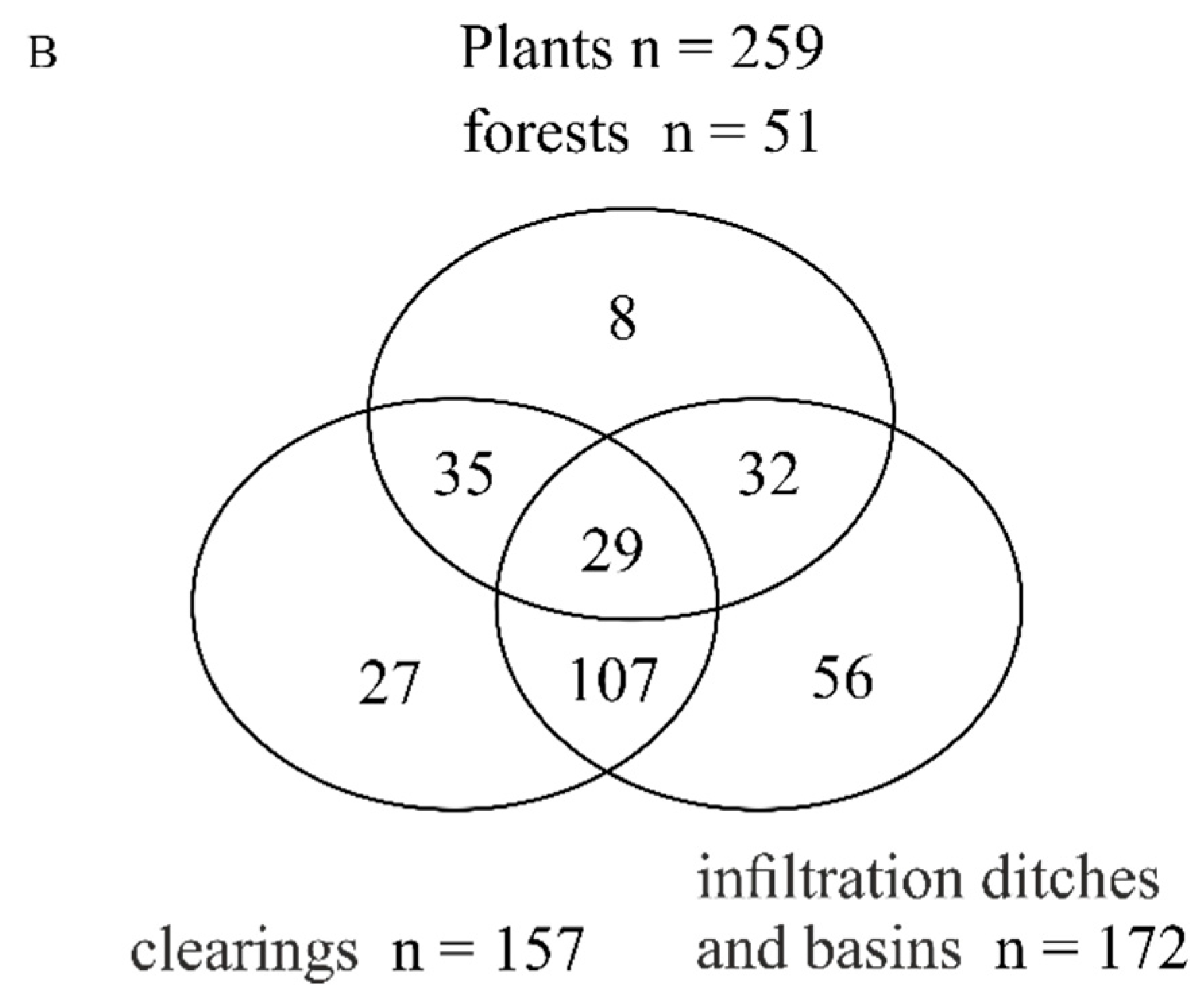
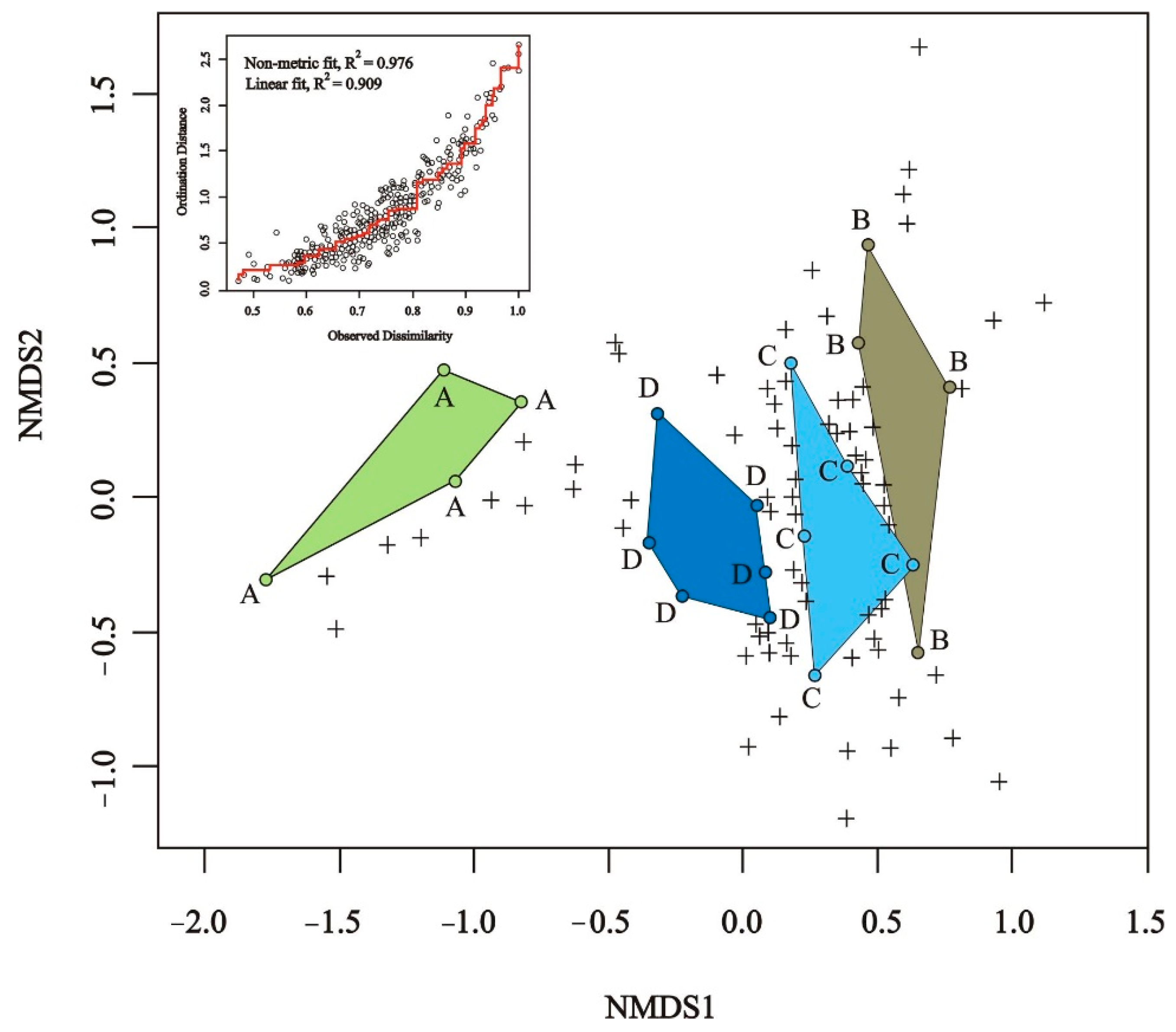
3.2. Bee Species Composition

The NMDS plot shows a clear division of bees from the 4 analysed types of habitats (non-metric fit, R² = 0.976; linear fit, R² = 0.909; stress = 0.156). The most distinct group was bees in forests, while the greatest similarity was observed between species caught in clearings and infiltration basins. Simultaneously, species found in basins are intermediate between these two clumps but more similar to bees in clearings and ditches than to forest species (Figure 3). The significance of habitat types for bee communities is presented in

Table 2. PERMANOVA results for wild bee and plant communities based on Bray–Curtis distances.

Variable	df	SS	MS	F	R2	p
	BEES
Habitat type	3	2.663	0.888	4.630	0.377	0.001
Residuals	23	4.410	0.192		0.623
Total	26	7.073			1
	PLANTS
Habitat type	7	3.448	0.493	3.877	0.337	0.001
Soil type (dry vs. wet)	1	2.722	2.722	21.433	0.266	0.001
Residuals	32	4.065	0.127		0.397
Total	40	10.235			1

df = degrees of freedom; SS = sum of squares; MSS = mean sum of squares. Bold estimates indicate significant effects at p < 0.05.

.

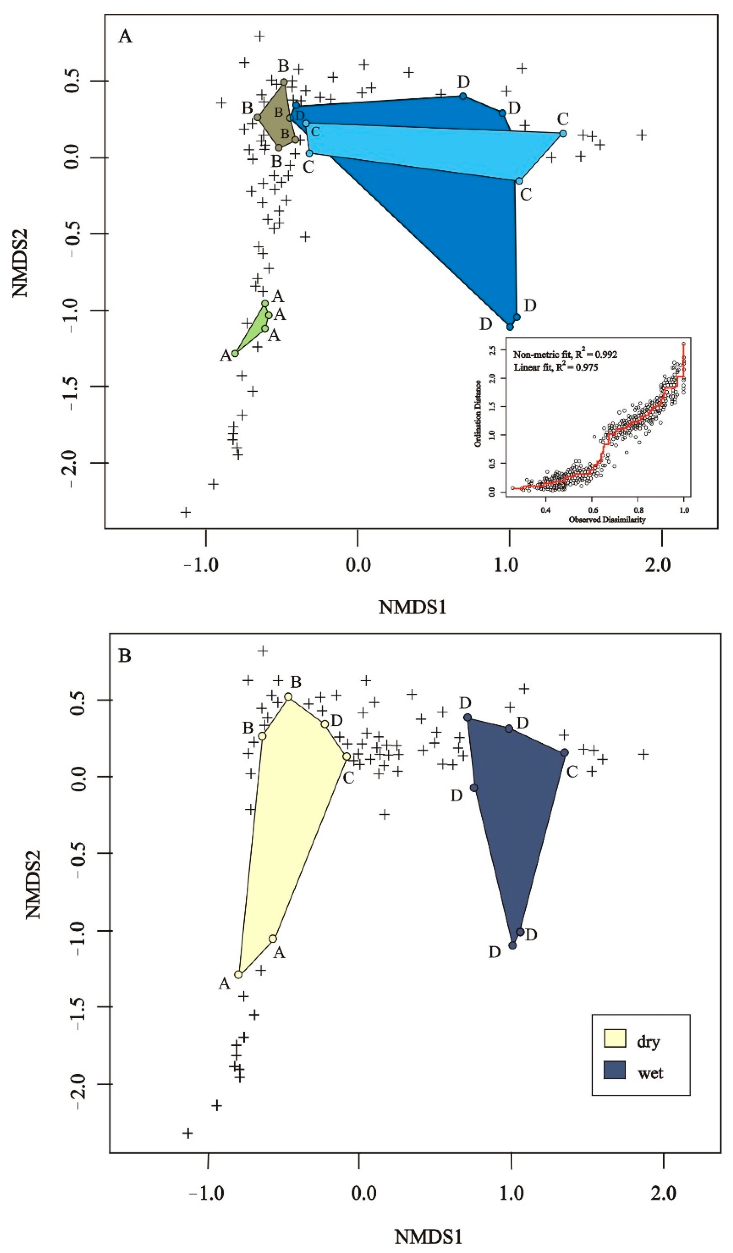
3.3. Plant Species Composition

NMDS plot shows a clear separation of the flora of forest communities (non-metric fit, R² = 0.992; linear fit, R² = 0.975; stress = 0.113) from the other groups, i.e., clearings, infiltration ditches, and basins (Figure 4A). The last 2 groups strongly overlap; in the case of dry habitats, they are indistinguishable (Figure 4A,B). When simultaneously comparing plant preferences in respect of moisture conditions, we observed a clear separation of species of dry habitats from those of wet habitats. This is also visible in Shepard diagrams as discontinuity between 2 groups of points (Figure 4A,B). The significance of habitat type and soil moisture content is shown in Table 2.

3.4. Changes in Bee Abundance and Species Richness

Species richness and abundance of bees in clearings, infiltration ditches and basins were higher than in forests. Similarly, higher species richness was observed in ditches and basins than in clearings. However, no significant differences were detected in bee species richness and abundance between ditches and infiltration basins and in abundance between clearings and both basins and ditches (

Table 3. Associations between habitat types (forests, clearings, infiltration ditches, infiltration basins) and bee species richness and abundance, based on generalized linear mixed models (GLMMs).

Habitat		Total Richness			Total Abundance
		Estimate ± SE	z	p	Estimate ± SE	z	p
Forests vs.	clearings	3.46 ± 1.19	7.04	<0.001	6.85 ± 1.17	12.31	<0.001
	ditches	4.50 ± 1.18	8.90	<0.001	7.60 ± 1.18	12.17	<0.001
	basins	5.00 ± 1.18	9.62	<0.001	6.29 ± 1.14	13.81	<0.001
Clearings vs.	ditches	1.30 ± 1.13	2.21	0.027	1.11 ± 1.21	0.55	0.583
	basins	1.44 ± 1.12	3.21	0.001	0.92 ± 1.22	0.45	0.741
Ditches vs.	basins	1.11 ± 1.10	1.05	0.293	0.83 ± 1.23	0.62	0.362

The models take into account spatial and temporal correlations among collected data; bold estimates indicate significant effects at p < 0.05.

).

The low species richness and abundance of species in forest habitats are reflected in the occurrence of bees of the distinguished functional groups. In respect of species richness and abundance in clearings, infiltration ditches, and basins, polylectic, cleptoparasitic, and soil- and cavity-nesting bees prevailed. A similar relationship was observed for the species richness of bees nesting above ground hives. In respect of abundance, hive-nesting bees prevailed in clearings and basins in comparison to forests. Simultaneously, in wooded habitats, no oligolectic species were caught.

We found, however, that in respect of species richness, infiltration basins were more attractive to polylectic and soil-nesting species than clearings were. In habitats of infiltration basins, higher species richness was recorded for species nesting in hives, while cavity-nesting species prevailed at the sites with infiltration ditches in terms of both species richness and abundance (

Table 4. Associations between habitat types (forests, clearings, infiltration ditches, infiltration basins) and species richness and abundance of bees differing in food preferences (polylectic, oligolectic, cleptoparasitic), based on generalized linear mixed models (GLMMs).

Habitat/ Functional Trait		Total Richness			Total Abundance
		Estimate ± SE	z	p	Estimate ± SE	z	p
POLYLECTIC
Forests vs.	clearings	2.39 ± 1.19	4.91	<0.001	5.54 ± 1.17	10.77	<0.001
	ditches	3.19 ± 1.18	7.03	<0.001	6.30 ± 1.18	10.87	<0.001
	basins	3.74 ± 1.18	8.08	<0.001	5.86 ± 1.14	13.41	<0.001
Clearings vs.	ditches	1.33 ± 1.12	2.60	0.009	1.14 ± 1.21	0.68	0.499
	basins	1.56 ± 1.11	4.14	<0.001	1.06 ± 1.21	0.30	0.764
Ditches vs.	basins	1.17 ± 1.09	1.87	0.061	0.95 ± 1.22	0.45	0.748
OLIGOLECTIC
Clearings vs.	ditches	1.28 ± 1.47	0.63	0.527	1.66 ± 1.62	1.04	0.297
	basins	1.33 ± 1.46	0.75	0.451	1.30 ± 1.59	0.57	0.568
Ditches vs.	basins	1.04 ± 1.38	0.12	0.903	0.67 ± 1.51	0.53	0.669
CLEPTOPARASITIC
Forests vs.	clearings	11.22 ± 1.83	3.99	<0.001	22.42 ± 1.93	4.73	<0.001
	ditches	15.91 ± 1.81	4.68	<0.001	24.20 ± 1.87	5.08	<0.001
	basins	15.08 ± 1.81	4.59	<0.001	23.29 ± 1.87	5.02	<0.001
Clearings vs.	ditches	1.42 ± 1.23	1.66	0.098	1.08 ± 1.45	0.21	0.836
	basins	1.34 ± 1.24	1.40	0.163	1.04 ± 1.45	0.10	0.919
Ditches vs.	basins	0.95 ± 1.18	−0.32	0.748	0.96 ± 1.37	−0.12	0.902

The models take into account spatial and temporal correlations among collected data; bold estimates indicate significant effects at p < 0.05.

and

Table 5. Associations between habitat types (forests, clearings, infiltration ditches, infiltration basins) and species richness and abundance of bees differing in nesting preferences (soil, hive, cavity) based on generalized linear mixed models (GLMMs).

Habitat/ Functional Trait		Total Richness			Total Abundance
		Estimate ± SE	z	p	Estimate ± SE	z	p
SOIL
Forests vs.	clearings	1.84 ± 1.26	2.66	0.008	6.39 ± 1.23	8.80	<0.001
	ditches	3.27 ± 1.23	5.67	<0.001	9.81 ± 1.29	8.93	<0.001
	basins	3.84 ± 1.23	6.54	<0.001	4.30 ± 1.16	10.02	<0.001
Clearings vs.	ditches	1.78 ± 1.18	3.48	<0.001	1.54 ± 1.35	1.43	0.154
	basins	2.09 ± 1.17	4.60	<0.001	0.67 ± 1.33	1.62	0.127
Ditches vs.	basins	1.17 ± 1.13	1.30	0.193	0.42 ± 1.35	2.88	0.005
HIVE
Forests vs.	clearings	3.15 ± 1.33	3.98	<0.001	13.54 ± 2.66	2.67	0.008
	ditches	2.19 ± 1.33	2.78	0.005	5.00 ± 3.27	1.36	0.174
	basins	3.70 ± 1.31	4.81	<0.001	13.56 ± 3.24	2.22	0.027
Clearings vs.	ditches	0.70 ± 1.19	−2.08	0.038	0.37 ± 2.60	−1.04	0.297
	basins	1.18 ± 1.17	1.04	0.300	1.00 ± 2.62	0	0.999
Ditches vs.	basins	1.69 ± 1.16	3.59	<0.001	2.71 ± 3.26	0.84	0.399
CAVITY
Forests vs.	clearings	20.77 ± 2.75	3.00	0.003	31.97 ± 2.87	3.29	0.001
	ditches	30.20 ± 2.72	3.41	0.001	112.25 ± 2.82	4.55	<0.001
	basins	19.42 ± 2.73	2.96	0.003	26.91 ± 2.84	3.15	0.002
Clearings vs.	ditches	1.45 ± 1.28	1.50	0.133	3.51 ± 1.56	2.83	0.005
	basins	0.94 ± 1.30	−0.26	0.798	0.84 ± 1.56	−0.39	0.662
Ditches vs.	basins	0.64 ± 1.24	−2.09	0.037	0.24 ± 1.49	−3.58	<0.001

The models take into account spatial and temporal correlations among collected data; bold estimates indicate significant effects at p < 0.05.

).

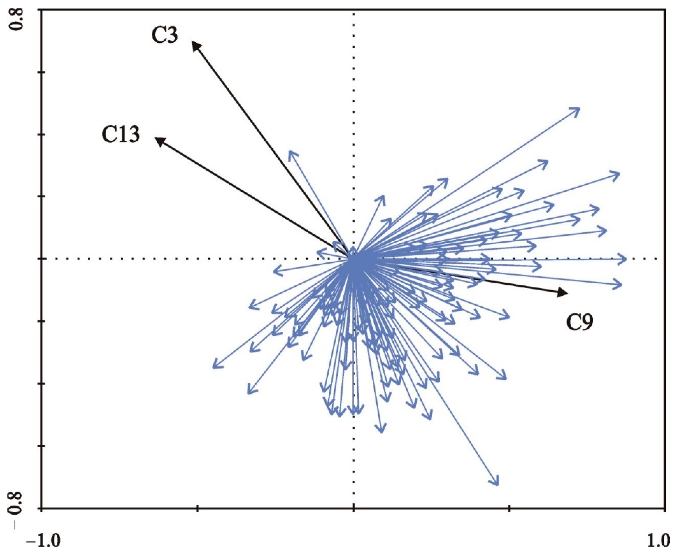
3.5. Factors Affecting Bee Species Richness and Abundance

Using redundancy analysis, we show that 3 variables significantly influenced bee occurrence. Increasing woody vegetation coverage (C3) and mean degree of shading during daytime (C13) affected it negatively. In contrast, the mean radius of a belt of predominantly open habitats around sampling sites (C9) had a positive impact. The other variables did not affect bee preferences significantly. All the variables used in the analysis explained 48.7% of the variation in Apiformes species data (sum of all canonical eigenvalues: 0.487; sum of all eigenvalues: 1.000; 0.487/1.000 = 0.487, i.e., 48.7%). Vector labels refer to significant variables (C3 = mean cover by woody species, C9 = mean radius of a belt of predominantly open habitats around sampling sites, C13 = mean degree of shading at daytime) (

Table 6. Results of stepwise selection of variables and a Monte Carlo permutation test—analysis of significance of effects of the studied variables on occurrence of different species of the Apiformes; variables were considered significant at p < 0.05.

Variable	RDA
	p	Variance	% of Explained Variance	VIF
C3 = mean cover by woody species	0.001	0.12	3.55	3.884
C9 = mean radius of a belt of predominantly open habitats around sampling sites	0.001	0.10	2.80	3.427
C13 = mean degree of shading at daytime	0.022	0.05	1.87	7.923
C14 = presence of water	0.105	0.05	1.44	1.494
C10 = site area (m2)	0.248	0.04	1.19	4.013
C11 = coefficient of border development	0.149	0.04	1.35	5.918
C12 = habitat barriers	0.320	0.03	1.13	3.884
C15 = presence of scarps	0.350	0.03	1.13	6.226
C7 = mean cover by plant species typical of dry soils	0.738	0.03	0.75	2.801

Less significant variables: C1 = mean plant cover (%, all plants); C2 = mean cover by flowering species; C4 = mean cover by herbaceous vegetation; C5 = mean cover by native plant species; C6 = mean cover by alien plant species; C8 = mean cover by plant species typical of wet soils, with others (VIF > 10) removed from RDA analysis; bold estimates indicate significant effects at p < 0.05.

, Figure 5).

4. Discussion

4.1. Infiltration Basins as New Habitats for Bees

Results of this study show that in wooded areas, industrial infrastructure can be crucial for the occurrence and increased abundance of species associated with open habitats. As far as we know, currently, little is known about this topic [13]. Considering the small spatial scale of our study, further research is needed. In this case, economic activity related to water purification for inhabitants of a European city has resulted in the creation of unique ecosystems, which are similar to post-extraction sites. Extraction of minerals leads to the formation of new habitats, often contrasting with the surrounding landscape, such as exposed surfaces, sandy and rocky walls, or water bodies [41]. Such disturbed areas often provide simultaneously various valuable habitats, such as wetlands or grasslands [69,70], which are rare and threatened in European landscapes. Thus, they increase the richness of the cultural landscape, i.e., shaped by human impact and, in this context, they are highly valuable for restoration ecology and conservation biology [39,41,43,44,71,72,73,74].

4.2. Changes in Natural Resources of Plants and Bees and Habitat Preferences of Species

We found that construction of infiltration basins in a pure pine forest stand growing on potential sites of pine-oak forest (in some places close to potential sites of open oak forest, evidenced by the presence of Potentilla alba L. and other thermophilous species, such as Anthericum ramosum L., Clinopodium vulgare L., Galium verum L. or Peucedanum oreoselinum (L.) Moench) has led to the exposure of bare soil, which resulted in an increased abundance of bee food plants and bees in the study area. Eventually, habitat type significantly affected species richness and abundance of species, which was the lowest in wooded habitats. As reported by other authors, the rate of colonization of newly created habitats by bees can be very fast [14,75,76], and the generated structure of the new bee community can be similar to that of communities in corresponding undisturbed habitats [77,78]. In our study, we could not assess the rate of their initial colonization because field research was started 8 years after the construction of infiltration basins. However, we observed a completely different structure of plant and bee communities in the new habitats as compared to the neighbouring wooded habitats. The construction of water bodies has enabled their colonization by species that were not observed in wooded habitats before. As many as 22% of plant species and 41% of bee species were recorded only in infiltration basins. In contrast, widely distributed species, i.e., those found in all habitat types, accounted for 11 and 10%, respectively. The low species richness of flora and fauna of wooded habitats is also reflected in the similarity of bee and plant communities. Our results show that among the four analysed habitat types (forests, clearings, infiltration ditches, and infiltration basins), forests were the most distinct. Considering bee communities exclusively, those recorded in clearings and infiltration ditches were very similar. This is most probably linked with the soil moisture level, resulting from the degree of shading during the daytime, which was conditioned by habitat type, its location in the landscape, and preferences of the species. The mean coverage of shaded parts in both places was similar: 46% in clearings and 30% in infiltration ditches, compared to only 10% in infiltration basins.

We found that an increase in woody vegetation coverage and the degree of shading during the daytime negatively affected bee occurrence. This can be explained in various ways. First, bees often prefer to forage in open habitats with a high level of solar radiation, which is particularly relevant with reference to solitary bees and the species nesting on the ground [79]. They usually have higher thermal requirements for flight activity and larval development, associated mostly with open or slightly shaded places [80,81]. Increasing coverage of woody vegetation is linked with strong shading, causing a higher moisture content. This relationship shows a negative trend in the context of bee preferences, but it can be modified by many factors, such as habitat heterogeneity, accessibility of bare soil, or abundance of food resources [75]. Moreover, an increase in coverage by trees lowers the density of the undergrowth and the abundance of blooming plants in the herbaceous and shrub layers when trees have leaves, and all of this makes them less attractive to bees [79,82]. Probably the negative effect of increasing tree coverage on bees also results from the techniques of sample collection [83], as in this study, no bee samples were collected in the tree layer. Furthermore, most of the trees in the studied wooded habitats were wind-pollinated and, hence, less attractive to bees.

It is assumed that higher plant diversity is linked with the diversity of wild bees [84]. Most probably, however, this relationship can be explained by a greater heterogeneity of habitats [85,86]. A high variation of microhabitats, resulting from a varied structure of vegetation and type of land use, is one of the factors favouring the occurrence of taxonomically and functionally varied species, which use different parts of habitats for nesting and foraging [87,88]. Deforestation, and thus decreasing the degree of shading of the habitats, positively affected bee occurrence (e.g., forests vs. clearings and infiltration basins or ditches vs. infiltration ponds). Simultaneously, earthworks contributed to increasing the species richness of bees nesting in the soil (infiltration basins vs. forests and clearings). However, this did not apply to their cleptoparasites. Among bees nesting in the ground, many species prefer permeable sandy soils, which dominated in the study area [89]. In contrast, the distribution of species nesting above the ground was conditioned, e.g., by the presence of herbaceous plants with hollow stems. Such species dominated the plant cover of infiltration ponds, which was reflected in higher bee species richness and abundance. The large number of stones used to stabilize escarpments of infiltration ditches could also be beneficial and contribute to increasing the species richness of hive-nesting bees.

Undoubtedly, the destruction of initial forest habitats has led to the appearance of empty ecological niches. This “emptiness” has attracted not only eurytopic species, with a broad ecological spectrum, which can easily adapt to given conditions, but also some specialized species. This is particularly relevant with reference to plants [90] that provide food resources for bees. However, in this study, we have not detected any significant differences in species richness and abundance of oligolectic bees between individual habitat types.

Partial and periodical filling of the basins with water has enabled their colonization by plants with various preferences with respect to soil moisture, which significantly influenced their occurrence according to the results of other studies [91,92]. The influence of soil on the habitat preference of plants is reflected in the plot of similarity, which shows a clear separation of species of dry habitats from those of wet ones. In Central Europe, soil moisture content—besides microclimate and soil pH—is one of the major factors shaping vegetation development [93].

One of the more important factors affecting bee diversity is the availability of suitable sites and substrates [94] used for nesting. Many of the bee species that nest in the ground prefer permeable sandy or loamy soils, which are typical of dry grasslands. Nevertheless, some studies show the attractiveness of moist meadows and other wet habitats [88,95,96]. The preferences of the Aculeata for humid sites are mostly due to dietary specialization rather than nesting site availability [97]. However, this topic is poorly studied, so it is difficult to find similar sets of habitats, which do not allow any detailed comparisons. The low availability of data probably results from an assumption that moist meadows are not suitable habitats for aculeates, supporting their high diversity. In contrast, our study confirms their attractiveness. We found that even periodical or only partial filling of infiltration basins with water did not limit the occurrence of bees. In spite of repeated flooding of the infiltration basins, the species richness and abundance of bees (including ground-nesting ones) were higher than in clearings and forests. This has probably resulted from the presence of sparsely vegetated places around the water bodies, which could be favourable nesting sites. The width of the belt of predominantly open habitats around the basins, where the soil was predominantly not under the canopy of trees (forests covering < 40% of total area), was a significant factor, positively affecting the occurrence of species. Moreover, the dense herbaceous cover of clearings, lacking places with bare soil, could limit the distribution of the Apiformes. Additionally, Stewart et al. [98] reported a positive effect of the immediate vicinity of water bodies in shaping the diversity of bees, indicating a significantly higher abundance of the Apiformes near the ponds as compared with control sites.

Contrary to our assumptions, we did not observe any significant effect of species richness and coverage by bee food plants on bee occurrence, although many researchers have considered them as some of the major factors influencing bee communities [11,99]. Hence, most probably, also in our research, nesting specialization has played a greater role in shaping bee preferences in the studied habitats than dietary specialization. A high abundance of bee food plants not only provides suitable food resources but also helps to increase the species richness of bees [100]. In our research, it was not a factor limiting the occurrence of the Apiformes, which probably resulted from a similar abundance of bee food plants in all the studied habitats (except for forests) and a high degree of taxonomic similarity of the plant cover of open habitats. For example, the mean cover by blooming species, mostly herbaceous species, reached 3.60% in clearings, 3.83% in ditches, and 3.66% in infiltration basins. In wooded habitats, this value was significantly higher (7.64%) but resulted from the high contribution of woody plants. They provided an abundant but very short-term source of food for bees in contrast to open habitats, which provided them with food throughout the growing season [19]. Moreover, trees were pollinated by only a small number of bee species.

Some urbanized and post-industrial localities are examples of habitats subject to dynamic successional transformations. In the present study, a hybrid ecosystem was formed as a result of the modification of the natural habitat. This ecosystem is capable of returning to the initial (historical) state when human impact ceases [101]. Undoubtedly, a lack of active measures for the management of open habitats facilitates their gradual transformation into wooded habitats [70]. The rate of succession depends on habitat quality. Succession on fertile and moist sites is faster than on poor, dry, and sandy soils [102]. At the investigated sites, successional processes are successively hampered by economic activity, resulting from land use in the area of infiltration basins and the demand for water for inhabitants of the city of Bydgoszcz. Irregular filling of the basins with water and their conservation by mowing of vegetation and ploughing of the surface of basins or felling of trees and shrubs, which have spontaneously colonized the basins and their immediate neighbourhood, markedly limit succession. Thus, these practices enable the development of taxonomically and functionally diverse groups of plants and bees. Moreover, on the landscape scale, they will increase bee diversity in urban forest ecosystems.

5. Conclusions

The presented results indicate that artificial, small water bodies located in highly isolated forest habitats play an important role in increasing bee species richness and abundance. They also create conditions for the coexistence of specialized plant species (hygrophilous vs. thermophilous). Although they are not typical habitats for pollinators, they should be classified as potential sites of a high diversity of the Aculeata. A special role is played by the edges of wetlands and water bodies. Properly managed shores and their immediate vicinity can provide not only bee forage but also suitable nesting sites. This is particularly important in the face of progressive climate change and the role of blue-green infrastructure in urban areas.

References

1. Grimm, N.B.; Faeth, S.H.; Golubiewski, N.E.; Redman, C.L.; Bai, J.; Wu, X.; Briggs, J.M. Global change and the ecology of cities. Science 2008, 319, 756–760. [Google Scholar] [CrossRef] [PubMed]
2. Somme, L.; Moquet, L.; Quinet, M.; Vanderplanck, M.; Michez, D.; Lognay, G.; Jacquemart, A.-L. Food in a row: Urban trees offer valuable floral resources to pollinating insects. Urban Ecosyst. 2016, 19, 1149–1161. [Google Scholar] [CrossRef]
3. Potts, S.G.; Biesmeijer, J.C.; Kremen, C.; Neumann, P.; Schweiger, O.; Kunin, W.E. Global pollinator declines: Trends, impacts and drivers. Trends Ecol. Evol. 2010, 25, 345–353. [Google Scholar] [PubMed]
4. Kowarik, I. Novel urban ecosystems, biodiversity, and conservation. Environ. Pollut. 2011, 159, 1974–1983. [Google Scholar] [CrossRef]
5. Sattler, T.; Obrist, M.K.; Duelli, P.; Moretti, M. Urban arthropod communities: Added value or just a blend of surrounding biodiversity? Landsc. Urban Plan. 2011, 103, 347–361. [Google Scholar] [CrossRef]
6. Beninde, J.; Veith, M.; Hochkirch, A. Biodiversity in cities needs space: A meta-analysis of factors determining intraurban biodiversity variation. Ecol. Lett. 2015, 18, 581–592. [Google Scholar]
7. Theodorou, P.; Radzevičiūtė, R.; Lentendu, G.; Kahnt, B.; Husemann, M.; Bleidorn, C.; Settele, J.; Schweiger, O.; Grosse, I.; Wubet, T.; et al. Urban areas as hotspots for bees and pollination but not a panacea for all insects. Nat. Commun. 2020, 11, 576. [Google Scholar] [CrossRef] [PubMed]
8. Normandin, É.; Vereecken, N.J.; Buddle, C.M.; Fournier, V. Taxonomic and functional trait diversity of wild bees in different urban settings. PeerJ 2017, 5, e3051. [Google Scholar]
9. Potts, S.G.; Imperatriz-Fonseca, V.; Ngo, H.T.; Aizen, M.A.; Biesmeijer, J.C.; Breeze, T.D.; Dicks, L.V.; Garibaldi, L.A.; Hill, R.; Settele, J.; et al. Safeguarding pollinators and their values to human well-being. Nature 2016, 540, 220–229. [Google Scholar]
10. Steffan-Dewenter, I.; Tscharntke, T. Resource overlap and possible competition between honey bees and wild bees in central Europe. Oecologia 2000, 1222, 288–296. [Google Scholar] [CrossRef]
11. Kearns, C.A.; Oliveras, D.M. Environmental factors affecting bee diversity in urban and remote grassland plots in Boulder, Colorado. J. Insect Conserv. 2009, 13, 655–665. [Google Scholar]
12. Buchholz, S.; Gathof, A.K.; Grossmann, A.J.; Kowarik, I.; Fischer, L.K. Wild bees in urban grasslands: Urbanisation, functional diversity and species traits. Landsc. Urban Plan. 2020, 196, 103731. [Google Scholar]
13. Twerd, L.; Sobieraj-Betlińska, A.; Szefer, P. Roads, railways, and power lines: Are they crucial for bees in urban woodlands? Urban For. Urban Green. 2021, 61, 127120. [Google Scholar]
14. Potts, S.G.; Vulliamy, B.; Dafni, A.; Ne’eman, G.; O’Toole, C.; Roberts, S.; Willmer, P. Response of plant-pollinator communities to fire: Changes in diversity, abundance and floral reward structure. Oikos 2003, 101, 103–112. [Google Scholar]
15. Tommasi, D.; Miro, A.; Higo, H.A.; Winston, M.L. Bee diversity and abundance in an urban setting. Can. Entomol. 2004, 136, 851–869. [Google Scholar]
16. Larson, J.L.; Kesheimer, A.J.; Potter, D.A. Pollinator assemblages on dandelions and white clover in urban and suburban lawns. J. Insect Conserv. 2014, 18, 863–873. [Google Scholar] [CrossRef]
17. Hicks, D.M.; Ouvrard, P.; Baldock, K.C.R.; Mark, M.; Goddard, A.; Kunin, W.E.; Mitschunas, N.; Memmott, J.; Morse, H.; Nikolitsi, M.; et al. Food for pollinators: Quantifying the nectar and pollen resources of urban flower meadows. PLoS ONE 2016, 11, e0158117. [Google Scholar]
18. Martins, K.T.; Gonzales, A.; Lechowicz, M.J. Patterns of pollinator turnover and increasing diversity associated with urban habitats. Urban Ecosyst. 2017, 20, 1359–1371. [Google Scholar]
19. Twerd, L.; Banaszak-Cibicka, W.; Sobieraj-Betlińska, A.; Waldon-Rudzionek, B.; Hoffmann, R. Contributions of phenological groups of wild bees as an indicator of food availability in urban wastelands. Ecol. Indic. 2021, 126, 107616. [Google Scholar] [CrossRef]
20. Haaland, C.; Gyllin, M. Butterflies and bumblebees in greenways and sown wildflower strips in Southern Sweden. J. Insect Conserv. 2010, 14, 125–132. [Google Scholar] [CrossRef]
21. Matteson, K.C.; Langellotto, G.A. Determinates of inner city butterfly and bee species richness. Urban Ecosyst. 2010, 13, 333–347. [Google Scholar]
22. Gunnarsson, B.; Federsel, L.M. Bumble bees in the city: Abundance, species richness and diversity in two urban habitats. J. Insect Conserv. 2014, 18, 1185–1191. [Google Scholar]
23. Ellis, E.C.; Antill, E.C.; Kreft, H. All is not loss: Plant biodiversity in the anthropocene. PLoS ONE 2012, 7, e30535. [Google Scholar]
24. Smith, R.M.; Thompson, K.; Hodgson, J.G.; Warren, P.H.; Gaston, K.J. Urban domestic gardens (IX): Composition and richness of the vascular plant flora, and implications for native biodiversity. Biol. Conserv. 2006, 129, 312–322. [Google Scholar]
25. Bartomeus, I.; Fründ, J.; Williams, N.M. Invasive plants as novel food resources, the pollinators’ perspective. In Biological Invasions and Animal Behavior; Weis, J.S., Sol, D., Eds.; Cambridge University Press: Cambridge, UK, 2016; pp. 119–132. [Google Scholar]
26. Matteson, K.C.; Langellotto, G.A. Small scale additions of native plants fail to increase beneficial insect richness in urban gardens. Insect Conserv. Divers. 2011, 4, 89–98. [Google Scholar]
27. Hanley, M.E.; Awbi, A.J.; Franco, M. Going native? Flower use by bumblebees in English urban gardens. Ann. Bot. 2014, 113, 799–806. [Google Scholar] [CrossRef]
28. Stewart, A.B.; Sritongchuay, T.; Teartisup, P.; Kaewsomboon, S.; Bumrungsri, S. Habitat and landscape factors influence pollinators in a tropical megacity, Bangkok, Thailand. PeerJ 2018, 6, e5335. [Google Scholar]
29. Shochat, E.; Lerman, S.B.; Anderies, J.M.; Warren, P.S.; Faeth, S.H.; Nilon, C.H. Invasion, competition, and biodiversity loss in urban ecosystems. BioScience 2010, 60, 199–208. [Google Scholar] [CrossRef]
30. Herzon, I.; Helenius, J. Agricultural drainage ditches, their biological importance and functioning. Biol. Conserv. 2008, 141, 1171–1183. [Google Scholar]
31. Hopwood, J.L. The contribution of roadside grassland restorations to native bee conservation. Biol. Conserv. 2008, 141, 2632–2640. [Google Scholar] [CrossRef]
32. Hopwood, J.; Winkler, L.; Deal, B.; Chivvis, M. Use of Roadside Prairie Plantings by Native Bees; Living Roadway Trust Fund. 2010. Available online: www.academia.edu/16996737/Use_of_roadside_prairie_plantings_by_native_bees (accessed on 15 October 2021).
33. Moroń, D.; Skórka, P.; Lenda, M.; Rożej-Pabijan, E.; Wantuch, M.; Kajzer-Bonk, J.; Celary, W.; Mielczarek, Ł.E.; Tryjanowski, P. Railway embankments as new habitat for pollinators in an agricultural landscape. PLoS ONE 2014, 9, e101297. [Google Scholar] [CrossRef]
34. Heneberg, P.; Bogusch, P.; Řezáč, M. Off-road motorcycle circuits support long-term persistence of bees and wasps (Hymenoptera: Aculeata) of open landscape at newly formed refugia within otherwise afforested temperate landscape. Ecol. Eng. 2016, 93, 187–198. [Google Scholar] [CrossRef]
35. Hill, B.; Bartomeus, I. The potential of electricity transmission corridors in forested areas as bumblebee habitat. R. Soc. Open Sci. 2016, 3, 160525. [Google Scholar] [CrossRef]
36. Heneberg, P.; Bogusch, P.; Řezáč, M. Roadside verges can support spontaneous establishment of steppe-like habitats hosting diverse assemblages of bees and wasps (Hymenoptera: Aculeata) in an intensively cultivated central European landscape. Biodivers. Conserv. 2017, 26, 843–864. [Google Scholar] [CrossRef]
37. Moroń, D.; Tryjanowski, P.; Celary, W.; Lenda, M.; Skórka, P. Railway lines affect spatial turnover of pollinator communities in an agricultural landscape. Biodivers. Res. 2017, 23, 1090–1097. [Google Scholar] [CrossRef]
38. Wagner, D.L.; Metzler, K.J.; Frye, H. Importance of transmission line corridors for conservation of native bees and other wildlife. Biol. Conserv. 2019, 235, 147–156. [Google Scholar] [CrossRef]
39. Krauss, J.; Alfert, T.; Steffan-Dewenter, I. Habitat area but not habitat age determines wild bee richness in limestone quarries. J. Appl. Ecol. 2009, 46, 194–202. [Google Scholar] [CrossRef]
40. Tropek, R.; Spitzer, L.; Konvicka, M. Two groups of epigeic arthropods differ in colonising of piedmont quarries: The necessity of multi-taxa and life-history traits approaches in the monitoring studies. Community Ecol. 2008, 9, 177–184. [Google Scholar] [CrossRef]
41. Tropek, R.; Kadlec, T.; Karesova, P.; Spitzer, L.; Kocarek, P.; Malenovsky, I.; Banar, P.; Tuf, I.H.; Hejda, M.; Konvicka, M. Spontaneous succession in limestone quarries as an effective restoration tool for endangered arthropods and plants. J. Appl. Ecol. 2010, 47, 139–147. [Google Scholar] [CrossRef]
42. Heneberg, P.; Bogusch, P.; Řehounek, J. Sandpits provide critical refuge for bees and wasps (Hymenoptera: Apocrita). J. Insect Conserv. 2013, 17, 473–490. [Google Scholar] [CrossRef]
43. Twerd, L.; Banaszak-Cibicka, W.; Sandurska, E. What features of sand quarries affect their attractiveness for bees? Acta Oecol. 2019, 96, 56–64. [Google Scholar] [CrossRef]
44. Twerd, L.; Szefer, P.; Sobieraj-Betlińska, A.; Olszewski, P. The conservation value of Aculeata communities in sand quarries changes during ecological succession. Glob. Ecol. Conserv. 2021, 28, e01693. [Google Scholar] [CrossRef]
45. Twerd, L. Ecology of Wild Bees (Hymenoptera: Apoidea: Apiformes) in the Conditions Influence of the Soda Industry; Wydawnictwo Uniwersytetu Kazimierza Wielkiego: Bydgoszcz, Poland, 2020; pp. 1–258. [Google Scholar]
46. Boroń, M.; Brodziak, R.; Bylka, J.; Sozański, M.M.; Urbaniak, A. The methodical concept for operation control of infiltration water intake. Ochr. Sr. 2015, 37, 29–33. [Google Scholar]
47. Banaszak, J. Studies on methods of censusing the numbers of bees (Hymenoptera, Apoidea). Pol. Ecol. Stud. 1980, 6, 355–366. [Google Scholar]
48. Geslin, B.; Le Féon, V.; Kuhlmann, M.; Vaissière, B.E.; Dajoz, I. The bee fauna of large parks in downtown Paris, France. Ann. Soc. Entomol. Fr. 2016, 51, 487–493. [Google Scholar] [CrossRef]
49. Bossert, S. Recognition and identification of bumblebee species in the Bombus lucorum-complex (Hymenoptera, Apidae)—A review and outlook. Dtsch. Entomol. Z. 2015, 62, 19–28. [Google Scholar] [CrossRef]
50. Wolf, S.; Rohde, M.; Moritz, R.F.A. The reliability of morphological traits in the differentiation of Bombus terrestris and B. lucorum (Hymenoptera: Apidae). Apidologie 2010, 41, 45–53. [Google Scholar] [CrossRef]
51. Banaszak, J.; Twerd, L. Importance of thermophilous habitats for protection of wild bees (Apiformes). Community Ecol. 2018, 19, 239–247. [Google Scholar] [CrossRef]
52. Banaszak-Cibicka, W.; Twerd, L.; Fliszkiewicz, M.; Giejdasz, K.; Langowska, A. City parks vs. natural areas—is it possible to preserve a natural level of bee richness and abundance in a city park? Urban Ecosyst. 2018, 21, 599–613. [Google Scholar] [CrossRef] [Green Version]
53. Barkman, J.J.; Doing, H.; Segal, S. Kritische Bemerkungen und Vorschläge zur quantitativen Vegetationsanalyse. Acta Bot. Neerl. 1964, 13, 394–419. [Google Scholar] [CrossRef]
54. Rutkowski, L. Klucz Do Oznaczania Roślin Naczyniowych Polski Niżowej; Wydawnictwo Naukowe PWN: Warszawa, Poland, 2004; pp. 1–816. [Google Scholar]
55. Mirek, Z.; Piękoś-Mirkowa, H.; Zając, A.; Zając, M. Flowering plants and pteridophytes of Poland. A checklist. In Biodiversity of Poland; Mirek, Z., Ed.; W. Szafer Institute of Botany, Polish Academy of Sciences: Kraków, Poland, 2002; Volume 1, pp. 1–442. [Google Scholar]
56. Ellenberg, H.; Weber, H.E.; Düll, R.; Wirth, V.; Werner, W.; Paulissen, D. Zeigerwerte von Pflanzen in Mitteleuropa. Scr. Geobot. 1992, 18, 1–258. [Google Scholar]
57. QGIS 2.18.21 Essen Development Team. QGIS: A Free and Open-Source Geographic Information System; Open-Source Geospatial Foundation Project. Available online: Qgis-polska.org/pliki (accessed on 25 April 2021).
58. Kujawa, K. Wpływ Struktury Zadrzewień Oraz Struktury Krajobrazu Rolniczego na Zgrupowania Ptaków Lęgowych w Zadrzewieniach; Akademia Rolnicza im. Augusta Cieszkowskiego w Poznaniu: Poznań, Poland, 2006; pp. 1–160. [Google Scholar]
59. Bhattacharya, M.; Primack, R.B.; Gerwein, J. Are roads and railroads barriers to bumblebee movement in a temperate suburban conservation area? Biol. Conserv. 2003, 109, 37–45. [Google Scholar] [CrossRef]
60. Farwig, N.; Bailey, D.; Bochud, E.; Herrmann, J.D.; Kindler, E.; Reusser, N.; Schüepp, C.; Schmidt-Entling, M.H. Isolation from forest reduces pollination, seed predationand insect scavenging in Swiss farmland. Landsc. Ecol. 2009, 24, 919–927. [Google Scholar] [CrossRef]
61. Fischer, L.K.; Eichfeld, J.; Kowarik, I.; Buchholz, S. Disentangling urban habitat and matrix effects on wild bee species. PeerJ 2016, 4, e2729. [Google Scholar] [CrossRef] [PubMed]
62. Gotelli, N.J.; Colwell, R.K. Quantifying biodiversity: Procedures and pitfalls in measurement and comparison of species richness. Ecol. Lett. 2001, 4, 379–391. [Google Scholar] [CrossRef]
63. Colwell, R.K. EstimateS: Statistical Estimation of Species Richness and Shared Species from Sample; User’s Guide and Applications. 2006. Available online: Purl.oclc.org/estimates (accessed on 15 August 2021).
64. Chao, A. Non-parametric estimation of the number of classes in a population. Scand. J. Stat. 1984, 11, 265–270. [Google Scholar]
65. Oksanen, J.; Blanchet, F.G.; Kindt, R.; Legendre, P.; O’Hara, R.B.; Simpson, G.L.; Solymos, P.; Stevens, M.H.H.; Wagner, H. Package ‘Vegan’. Community Ecology Package. R Package. 2011. Available online: Cran.r-project.org/package=vegan (accessed on 5 October 2021).
66. R Development Core Team. R: A Language and Environment for Statistical Computing; R Foundation for Statistical Computing: Vienna, Austria, 2021. [Google Scholar]
67. Bates, D.; Maechler, M.; Bolker, B. Fitting linear mixed-effects models using lme4. J. Stat. Softw. 2015, 67, 1–48. [Google Scholar] [CrossRef]
68. ter Braak, C.J.F.; Šmilauer, P. CANOCO Reference Manual and User’s Guide to Canoco for Windows; Software for Canonical Community Ordination; Microcomputer Power: Ithaca, NY, USA, 1998. [Google Scholar]
69. Novák, J.; Prach, K. Vegetation succession in basalt quarries: Pattern on a landscape scale. Appl. Veg. Sci. 2003, 6, 111–116. [Google Scholar] [CrossRef]
70. Trnková, R.; Řehounková, K.; Prach, K. Spontaneous succession of vegetation on acidic bedrock in quarries in the Czech Republic. Preslia 2010, 82, 333–343. [Google Scholar]
71. Brändle, M.; Durka, W.; Altmoos, M. Diversity of surface dwelling beetle assemblages in open-cast lignite mines in Central Germany. Biodiver. Conserv. 2000, 9, 1297. [Google Scholar] [CrossRef]
72. Tichanek, F.; Tropek, R.J. Conservation value of post-mining headwaters: Drainage channels at a lignite spoil heap harbour threatened stream dragonflies. J. Insect Conserv. 2015, 19, 975. [Google Scholar] [CrossRef]
73. Harabis, F. High diversity of odonates in post-mining areas: Meta-analysis uncovers potential pitfalls associated with the formation and management of valuable habitats. Ecol. Eng. 2016, 90, 438–446. [Google Scholar] [CrossRef]
74. Hodecek, J.; Kuras, T.; Šipoš, J.; Dolný, A. Post-industrial areas as successional habitats: Long-term changes of functional diversity in beetle communities. Basic Appl. Ecol. 2015, 16, 629–640. [Google Scholar] [CrossRef]
75. Steffan-Dwenter, I.; Tscharntke, T. Succession of bee communities on fallows. Ecography 2001, 24, 83–93. [Google Scholar] [CrossRef]
76. Griffin, S.R.; Bruninga-Socolar, B.; Morgan, A.; Kerr, M.A.; Gibbs, J.; Winfree, R. Wild bee community change over a 26-year chronosequence of restored tallgrass prairie. Restor. Ecol. 2016, 25, 650–660. [Google Scholar] [CrossRef]
77. Exeler, N.; Kratochwil, A.; Hochkirch, A. Restoration of riverine inland sand dune complexes: Implications for the conservation of wild bees. J. Appl. Ecol. 2009, 46, 1097–1105. [Google Scholar] [CrossRef]
78. Tarrant, S.; Ollerton, J.; Rahman, M.L.; Tarrant, J.; McCollin, D. Grassland restoration on landfill sites in the East Midlands, United Kingdom: An evaluation of floral resources and pollinating insects. Restor. Ecol. 2013, 21, 560–568. [Google Scholar] [CrossRef]
79. McKinney, A.M.; Goodell, K. Shading by invasive shrub reduces seed production and pollinator services in a native herb. Biol. Invasions. 2010, 12, 2751–2763. [Google Scholar] [CrossRef]
80. Osborne, J.L.; Williams, I.H.; Corbet, S.A. Bees, pollination and habitat change in the European community. Bee World 1991, 72, 99–116. [Google Scholar] [CrossRef]
81. Cane, J.H.; Tepedino, V.J. Causes and extent of declines among native North American invertebrate pollinators: Detection, evidence, and consequences. Conserv. Ecol. 2001, 5, 1. [Google Scholar] [CrossRef]
82. Wulf, M.; Naaf, T. Herb layer response to broadleaf tree species with different leaf litter quality and canopy structure in temperate forests. J. Veg. Sci. 2009, 20, 517–526. [Google Scholar] [CrossRef]
83. Wu, P.; Axmacher, J.C.; Song, X.; Zhang, X.; Xu, H.; Chen, C.; Yu, Z.; Liu, Y. Effects of plant diversity, vegetation composition, and habitat type on different functional trait groups of wild bees in rural Beijing. J. Insect Sci. 2018, 18, 4. [Google Scholar] [CrossRef] [PubMed] [Green Version]
84. Huston, M. General hypothesis of species-diversity. Am. Nat. 1979, 113, 81–101. [Google Scholar] [CrossRef]
85. Haddad, N.M.; Tilman, D.; Haarstad, J.; Ritchie, M.; Knops, J.M.H. Contrasting effects of plant richness and composition on insect communities: A field experiment. Am. Nat. 2001, 158, 17–35. [Google Scholar] [CrossRef] [PubMed]
86. Hawkins, B.A.; Porter, E.E. Does herbivore diversity depend on plant diversity? The case of California butterflies. Am. Nat. 2003, 161, 40–49. [Google Scholar] [CrossRef]
87. Bogusch, P.; Blažej, L.; Trýzna, M.; Heneberg, P. Forgotten role of fires in Central European forests: Critical importance of early post-fire successional stages for bees and wasps (Hymenoptera: Aculeata). Eur. J. For. Res. 2015, 134, 153–166. [Google Scholar] [CrossRef]
88. Heneberg, P.; Bogusch, P.; Řezáč, M. Numerous drift sand “specialists” among bees and wasps (Hymenoptera: Aculeata) nest in wetlands that spontaneously form de novo in arable fields. Ecol. Eng. 2018, 117, 133–139. [Google Scholar] [CrossRef]
89. Cane, J.H. Soils of ground-nesting bees (Hymenoptera: Apoidea): Texture, moisture, cell depth and climate. J. Kans. Entomol. Soc. 1991, 64, 406–413. [Google Scholar]
90. Řehounková, K.; Prach, K. Spontaneous vegetation succession in disused gravel-sand pits: Role of local site and landscape factors. J. Veg. Sci. 2006, 17, 583–590. [Google Scholar] [CrossRef]
91. Walker, L.R.; del Moral, R. (Eds.) Primary Succession and Ecosystem Rehabilitation; Cambridge University Press: Cambridge, UK, 2003; pp. 1–442. [Google Scholar]
92. Prach, K.; Pysek, P.; Jarosık, V. Climate and pH as determinants of vegetation succession in Central European man-made habitats. J. Veg. Sci. 2007, 18, 701–710. [Google Scholar] [CrossRef]
93. Prach, K.; Řehounková, K.; Lencová, K.; Jírová, A.; Konvalinková, P.; Mudrák, O.; Študent, V.; Vaněček, Z.; Tichy, L.; Petřík, P.; et al. Vegetation succession in restoration of disturbed sites in Central Europe: The direction of succession and species richness across 19 seres. Appl. Veg. Sci. 2014, 17, 193–200. [Google Scholar] [CrossRef]
94. Potts, S.G.; Vulliamy, B.; Roberts, S.; O’Toole, C.; Dafni, A.; Ne’eman, G.; Willmer, P. Role of nesting resources in organising diverse bee communities in a Mediterranean landscape. Ecol. Entomol. 2005, 30, 78–85. [Google Scholar] [CrossRef]
95. Ziaja, M.; Denisow, B.; Wrzesień, M.; Wójcik, T. Availability of food resources for pollinators in three types of lowland meadows. J. Apic. Res. 2018, 57, 467–478. [Google Scholar] [CrossRef]
96. Vickruck, J.L.; Best, L.R.; Gavin, M.P.; Devries, J.H.; Galpern, P. Pothole wetlands provide reservoir habitat for native bees in prairie croplands. Biol. Conserv. 2019, 232, 43–50. [Google Scholar] [CrossRef]
97. Moroń, D.; Szentgyörgyi, H.; Wantuch, M.; Celary, W.; Westphal, C.; Settele, J.; Woyciechowski, M. Diversity of wild bees in wet meadows: Implications for conservation. Wetlands 2008, 28, 975. [Google Scholar] [CrossRef]
98. Stewart, R.I.A.; Andersson, G.K.S.; Brönmark, C.; Klatt, B.J.; Hansson, L.-A.; Zülsdorff, V.; Smith, H.G. Ecosystem services across the aquatic–terrestrial boundary: Linking ponds to pollination. Basic Appl. Ecol. 2017, 18, 13–20. [Google Scholar] [CrossRef]
99. Twerd, L.; Banaszak-Cibicka, W. Wastelands: Their attractiveness and importance for preserving the diversity of wild bees in urban areas. J. Insect Conserv. 2019, 23, 573–588. [Google Scholar] [CrossRef]
100. Banaszak-Cibicka, W.; Ratyńska, H.; Dylewski, Ł. Features of urban green space favourable for large and diverse bee populations (Hymenoptera: Apoidea: Apiformes). Urban For. Urban Green. 2016, 20, 448–452. [Google Scholar] [CrossRef]
101. Ejrnæs, R.; Hansen, D.N.; Aude, E. Changing course of secondary succession in abandoned sandy fields. Biol. Conserv. 2003, 109, 343–350. [Google Scholar] [CrossRef]
102. Hobbs, R.J.; Higgs, E.S.; Hall, C.A. (Eds.) Novel Ecosystems: Intervening in the New Ecological World Order; Wiley-Blackwell: Oxford, UK, 2013; pp. 1–384. [Google Scholar]
Figure 1. Location of sampling sites: forests (1–4), clearings (5–9), infiltration ditches (10–18), and infiltration basins (19–27).
Forests 13 01410 g001
Figure 2. Venn diagram presenting the richness of shared and exclusive (A) bee and (B) plant species.
Forests 13 01410 g002aForests 13 01410 g002b
Figure 3. Non-metric multidimensional scaling: diagram showing similarity (Bray–Curtis index) of wild bee community structure for 4 habitat types: A = forests (green); B = clearings (olive); C = infiltration ditches (sky-blue); D = infiltration basins (navy blue).
Forests 13 01410 g003
Figure 4. Non-metric multidimensional scaling (NMDS, stress-value = 0.125) diagram showing (A) = similarity (Bray–Curtis index) of plant community structure for 4 habitat types: A = forests (green); B = clearings (olive); C = infiltration ditches (sky-blue); D = infiltration basins (navy blue); (B) = distribution of species of dry and wet habitats: A = forests; B = clearings; C = infiltration ditches; D = infiltration basins.
Forests 13 01410 g004
Figure 5. Ordination diagram based on redundancy analysis of results from study sites with respect to the first 2 axes and vectors of significant variables.
Forests 13 01410 g005