Abstract
The hydroperiod determines the biogeochemical conditions and processes developing in the mangrove soil. Floods control the input of nutrients and the presence of regulators such as salinity and sulfides that, in high concentrations, degrade mangrove vegetation. This work aimed to determine biogeochemical and hydroperiod characteristics in natural and degraded mangrove conditions. Three sampling sites were placed along a spatial gradient, including fringe and basin mangroves with different conditions. Tree characteristics and biogeochemical variables (temperature, salinity, pH, redox potential, sulfides) were measured. The structural analysis indicated two conditions: undisturbed (Rhizophora mangle fringe and Avicennia germinans basin under natural conditions) and disturbed (degraded basin, with standing A. germinans tree trunks). The soil porewater salinity, concentration of sulfides, and temperature were significantly higher, and redox potential lower in the disturbed site. The fringe mangrove was permanently waterlogged with higher tides than the basin mangrove. There were more extended flooding periods on the degraded mangrove due to the loss of hydrological connection with the adjacent water body. Waterlogging in basin mangroves increased soil porewater salinity to 87.8 and sulfides to 153 mg L−1, causing stress and death in A. germinans mangroves. Our results show that the loss of hydraulic connectivity causes the chronic accumulation of salinity and sulfides, with consequences on tree metabolism, ultimately causing its death. It probably also involves the succession in microbial communities.
1. Introduction
Mangroves had evolved at the interface between sea and land [1]. They thrive in environments with high salinity and flooded soils, primarily by the entrance of seawater [2]. In these environments, mangroves develop aerial root structures with lenticels that allow for an oxidized rhizosphere, exclude salt through the root endodermis, and secrete salt through leaf glands [3,4]. Moreover, its location within the coastal zone provides ecosystem services to the society, such as protecting against wind and tidal surges caused by storms and hurricanes; it acts as a water filter, improving its quality. Furthermore, they host a great diversity of fish, crustaceans, aquatic marine and terrestrial vertebrates, and invertebrates [5].
Mangroves depend on the hydroperiod (level, frequency, and time of flooding) for their ecological functioning. The hydroperiod is the primary driver of biogeochemical and biological characteristics in mangroves; the properties of soil, the organic matter content, and flooding frequency control the microbial activity and, consequently, the sulfate cycle [6,7]. Natural or anthropic disturbances may cause prolonged periods of flooding or drought and consequently the alteration of the biogeochemical processes on which primary productivity, carbon stored, and nutrients availability rely [6,8,9,10,11].
Biogeochemical regulators respond to altered hydrologic conditions and stress vegetation, ultimately causing their death. Among those regulators affecting mangroves are salinity, temperature, pH, redox potential (Eh), and sulfide concentration. High porewater salinity concentration alters the competitive balance among species [12]. High temperature inhibits seedlings’ growth [13], while low temperature limits their survival and dissemination [14]. The soil redox potential (Eh) and pH indicate the system’s proportion of reducers and oxidants. They regulate many biogeochemical reactions that determine the stability of minerals and nutrients in the soil [13].
Furthermore, Eh influences the spatial distribution of mangroves due to species-specific tolerance to soil oxidation-reduction gradients [2], and sulfides have a toxic effect on plants, affecting metabolic and physiological processes and, ultimately, plant survival and growth [15]. Sulfides can degrade seagrass (Thalassia testudinum) leaves, decoupling photosynthesis and causing their death when concentrations exceed 16.03 mg L−1. In marsh vegetation (such as Spartina alterniflora communities) and mangroves, productivity declined when sulfide concentrations were higher than 32.06 mg L−1. Mangrove trees can tolerate higher concentrations of sulfides contrasting with seedlings [16], but it is unknown if this behavior is the same in a tidal regime for mangrove species.
In this sense, the hydroperiod gradients in wetlands have implications for the biogeochemical characteristics and consequences in the conservation or degradation of these systems. On a global scale, the mangrove degradation rate has risen to 35% over the last 20 years, and 62% of global losses between 2000–2016 resulted from land-use change [17,18]. In Mexico, 9.4% of mangrove cover (80,850 ha) was lost from 1970 to 2015 [19]. However, a local loss may be higher, such as in Isla del Carmen, Campeche, where 27% (1584 ha) of its original coverage is in an active degradation process. Hence, restoration programs are a priority. Evaluating the hydroperiod and biogeochemical characteristics is essential to achieve cost-effective interventions in the recovery of the coverage of these wetlands [20].
In Isla del Carmen, the degradation increased after hurricanes Roxana and Opal made landfall in 1995 [21]. The fall of trees by hurricane winds clogged the tidal creeks and affected their hydroperiod regime [6]. This research aims to determine the effect of flooding time on the mangrove biogeochemical characteristics, such as salinity concentrations, sulfides, and nutrients. In addition, we determined which regulator of porewater was associated with the hydrological degradation and death of tidal-dominated mangroves.
2. Materials and Methods
2.1. Study Area
Laguna de Términos is an extensive and shallow (average: 3.5 m) coastal lagoon in the Gulf of Mexico [22], located southwest of the Yucatan Peninsula in Campeche state, México. It is part of the Laguna de Términos Flora and Fauna Protection Area (LTFFPA), with about 750,000 ha, which encompasses a marine area and the largest coastal lagoon in Mexico. This region has mangroves, freshwater wetlands, submerged aquatic vegetation, lowland rainforest, palm groves, scrub vegetation, semi-deciduous forest, and coastal dune vegetation [23,24,25].
The study area is in Estero Pargo, north of Laguna de Términos lagoon, at Isla del Carmen, Campeche. Climate is tropical rainy with a mean of 26.7 °C and three climatic seasons: (i) dry, from February to April, (ii) rainy, from June to November; and (iii) cold and windy ‘nortes’, from December to February.
Mangrove communities are distributed according to tide variations [26], with minimum and maximum flooding as the two critical seasons: minimum flooding (from −0.24 m), with low rainfall and reduced riparian discharge, and maximum flooding, with high and extraordinary tides up to 0.92 m [27], low temperature, strong north winds, and moderate rainfall [6].
The mangroves from Estero Pargo form two central ecotypes: fringe and basin. The fringe mangrove is in direct contact with the main tidal creek, and it is a diverse community composed of R. mangle, A. germinans, and L. racemosa. Dominated by A. germinans, the basin mangrove is behind the fringe mangrove [28]. In Estero Pargo mangroves, total soil nitrogen ranges from 0.57% to 0.86% and total phosphorus from 0.06% to 0.04%, respectively, in the basin and fringe areas. Nevertheless, phosphorus limitation is higher in the basin area [29].
2.2. Sampling Design
Three sampling sites were established in the study area: the first site is on the fringe dominated by R. mangle. The second and third sites were set on a basin area dominated by A. germinans; one site was conserved, and another was disturbed, with about 90% of the dead trees (Figure 1). At each site, the vegetation structure was characterized by two-100 m2 plots. Furthermore, we measured the porewater temperature, redox potential salinity, sulfides, nutrients, soil density and organic matter, and hydroperiod (level, frequency, and flooding time).
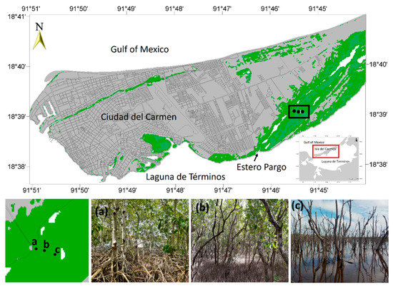
Figure 1.
Location of Estero Pargo mangrove in Ciudad del Carmen, Campeche, Mexico. (a) Fringe mangrove, (b) basin mangrove, and (c) impaired site.
2.2.1. Forest Structure
Structural attributes of mangroves were assessed at the beginning of the study. The forest structure of each site was determined, including adults, saplings, and seedlings. The height of seedlings and saplings was measured with a ruler, and a hypsometer was used to measure tree height. Diameter at Breast Height (DBH) was measured with calipers or a diameter tape. Individuals with a DBH of <2.5 cm and ≤50 cm height were considered seedlings; those with a DBH of <2.5 and height of >50 cm were considered saplings; and the rest (DBH > 2.5 and height > 50 cm) were considered trees. Plot sizes were 4 m2 for seedlings, 25 m2 for saplings, and 100 m2 for trees. We calculated basal area, density, and importance values index (IVI) based on these measurements. Finally, natural regeneration was estimated based on the number of seedlings and saplings per site [30,31,32].
2.2.2. Hydrology
At each site, the flooding regime at hourly intervals was determined with pressure sensors (Hobo U-20-001-01-Ti, Onset, Cape Cod, Massachusetts, USA) placed inside a 2 m long, 80 cm deep PVC tube. Pressure data were registered from April 2016 to December 2017 and converted to water levels, correcting for atmospheric pressure, and estimating water height, frequency, and flooding periods. The water level data were graphed as a scatterplot and smoothed using Lowess (Matlab, Mathworks, Natick, Mass, USA [33].
2.2.3. Biogeochemical Characteristics
- Soil porewater
Soil porewater samples at 35 cm depth were collected using a syringe and an acrylic tube [34]. Temperature, salinity, and pH were measured using a Myron 6P II Ultrameter. Additionally, we collected 200 mL pore water samples in plastic bottles, stored them in a cooler, and filtered them through Millipore filters of 0.22 µm. The methylene blue method was used to measure sulfide concentrations using a V-3000 field spectrophotometer (CHEMetrics Inc., Midland, VA, USA). Samples of nutrients (dissolved inorganic nitrogen (DIN = NH+4 + NO2− + NO3−) and soluble reactive phosphorus (SRP)) were fixed with chloroform and frozen until analysis. The nutrients were analyzed with a Skalar San Plus segmented flow autoanalyzer using the standard methods adopted from [35] and the circuits suggested by [36].
Soil potential redox (Eh) was measured with platinum electrodes and an Ag/AgCl reference electrode. The electrodes were placed at 0, 10, 20, and 30 cm deep, and the reference electrode was placed on the soil surface, 30 cm from the platinum electrode [34,37]. Due to the reference electrode potential, a correction factor of 235 mV was added to each reading [8]. These variables were determined in situ every two months from May 2016 to November 2017 (12 readings by each sampling).
- Soil
The soil bulk density and organic matter were determined by extracting two 30 cm deep cores from each plot. The sample was divided into three segments: 0–10 cm, 10–20 cm, and 20–30 cm, which were placed in a muffle at 60 °C for 72 h until constant weight [38]. The bulk density was calculated as dry soil weight divided by the volume of the sample [39]. The organic matter was determined with the loss of ignition method (calcination of matter) and calculated by the weight difference [40]. All variables were determined only once during the study.
2.2.4. Microtopography Transect
To characterize the microtopography we used the DGPS in static mode to set a benchmark in the impaired site (18.65096828 N, 91.757003738 W; and −0.106 masl referenced to WGS84) from a reference point (18.654027419 N, 91.761414738 W; and 1.1529 masl) [6]. Then, we set a total using a total station (Stonex STS2-R, Paderno Dugnano (MI), Italy) to trace a transect from the impaired site to the fringe [41]. We used a leveling staff in fixed reference points along the transect to measure soil elevation differences.
2.3. Analysis
Homoscedasticity and normality tests were performed on the data sets. Kruskal-Wallis (K-W) tests were used to determine the differences among sites and maximum and minimum flooding seasons for salinity, temperature, pH, Eh, sulfides, DIN and SRP [42]. A linear regression model was used to explore the relation between sulfide concentration and flooding time. These analyses were done on the InfoStat statistics program (professional version, Grupo Infostat, Ciudad de Córdoba, Argentina) [43].
According to the data distribution, Pearson or Spearman correlations were chosen to test the flooding period. The measured variables were analyzed using corrplot from the R ggcorrplot package [42]. The effect of the flooding on sulfide concentration, salinity, and Eh was determined through generalized linear models (GLMs), in which the independent variable was the number of days of flooding on the sampling sites, and the dependent variable was the concentration of these variables as limiting factors for the mangrove’s survival. These analyses were done in the statistical analysis software R 4.0.5 [44]. A 95% confidence interval was chosen to distinguish significantly different treatments.
3. Results
3.1. Forest Structure
Three species were recorded in the study area: R. mangle, A. germinans, and L. racemosa. The highest density and IVI were for A. germinans at the basin site (Table 1). At the same time, the dominant species in the fringe was R. mangle and the less abundant with the lowest values of all measured parameters (Table 1).

Table 1.
Forest structure of the study sites. There were no data on the impaired site because of the absence of live vegetation. Tre = Trees, Sap = Saplings, See = Seedling.
The recruiting of saplings and seedlings was similar in both sites (fringe: 5600 ind ha−1 and basin: 5300 ind ha−1). More saplings and seedlings of R. mangle were at the fringe than A. germinans and L. racemosa. There were no seedlings of L. racemosa, but their saplings were the tallest (1.21 ± 0.36 m). There were only seedlings and saplings of A. germinans in the basin, more abundant and taller than in the fringe mangrove (Table 1). Only dead trees were found at the impaired mangrove site, with no seedlings or saplings.
3.2. Flooding Levels and Hydroperiod
Two well-defined flooding periods were recorded: minimum (April to August 2016) and maximum (February to August 2017). The lowest flood levels (− 0.32 m) were recorded on the impaired mangrove in June 2016 and April 2017 (Figure 2). During this season, the flooding level decreased slowly in the impaired site, mainly in June 2016 and April 2017, contributing to an extension of the flooding period and waterlogging related to the loss of hydrological connectivity (Figure 2).
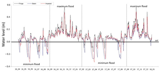
Figure 2.
Time series of water levels on the fringe, basin, and impaired basin, from April 2016 to December 2017. Periods by segments of the maximum and minimum floods or water levels are indicated.
Maximum floods were recorded from September 2016 to January 2017 and September to December 2017 (Figure 2). The highest flooding level (+0.58 m) was recorded at the mangrove fringe (November 2016 and October 2017). The flooding levels were similar on the three sites, evidencing the tide signal.
Significant differences were found among the study sites in the hydroperiod (K-W test, χ2 = 7.6; p = 0.009). The highest values of the three hydroperiod components were recorded at the fringe site, followed by the impaired, and finally by the basin site (Figure 3). The variation of the flooding level matched the occurrence of maximum and minimum floodings. For example, the maximum average flooding level (0.31 m) was recorded in October 2017 at the fringe mangrove. On the other hand, the lowest average flooding level (0.04 m) occurred during April and July 2017 in the mangrove basin and the impaired site (Figure 3a).

Figure 3.
Characteristics of the hydroperiod, (a) average level, (b) time, and (c) flooding frequency; black bars and circles, fringe mangrove; blue bars and circles, basin mangrove; red bars and circles, impaired basin mangrove.
The most prolonged flooding period occurred during the maximum flooding cycle on the three study sites. The average value of the flooding period was 730 hours month−1. The impaired site remained flooded for 733 hours month−1, followed by the basin (729 hours month−1) and the fringe (727 hours month−1) mangroves. During the minimum flooding season, mangroves were inundated for 525 hours month−1. The fringe site remained with the most prolonged average flooding period (583 h per month−1), followed by the impaired (511 hours month−1) and the basin site (480 hours month−1). During the whole study period at the impaired site, the minimum flooding time was 312 hours month−1 (Figure 3b).
The fringe mangrove presented an average flooding frequency of five tides month−1, followed by the impaired (2.5 tides month−1) and the basin sites (1.6 tides month−1). The lowest flooding frequency was recorded at the maximum flooding season on the three study sites, indicating that the mangrove remained flooded for most of the month. The average flooding frequency was 1.2 tides month−1 during the maximum flooding season. There were 1.6 tides month−1 in the fringe mangrove this season, followed by the impaired and the basin sites with one tide month−1. The average flooding frequency was 4.4 tides month−1 at the minimum flooding season. The highest flooding frequency was 7.8 tides month−1 at the fringe, 3.7 tides month−1 in the impaired site, and two tides month−1 in the basin site.
3.3. Biogeochemical Characteristics of Porewater
3.3.1. Spatio-Temporal
There were significant differences among sites in porewater salinity (χ2 = 79, p = 0.0001), with an increasing trend from the fringe to the basin and the impaired sites (mean ± s.d. = 37.9 ± 1.0, 65.1 ± 0.7, 71.1 ± 1.3 respectively, Figure 4a). The temperature was significantly higher in the impaired site than in the fringe and conserved basin sites (K-W test, χ2 = 24, p < 0.0001; Figure 4b).

Figure 4.
Temporal variation (mean ± SD) of (a) salinity, (b) temperature, (c) sulfide, (d) Eh, (e) dissolved inorganic nitrogen (DIN), and (f) soluble reactive phosphorus (SRP) in the fringe (triangles), basin (circles), and impaired (squares) mangrove sites.
Sulfide concentration was also significantly higher in the impaired site (70.2 ± 3.4 mg L−1) than in the fringe and basin sites (16.3 ± 3.2 mg L−1; K-W test, χ2 = 58, p = 0.0001; Figure 4c). The DIN was significantly higher in the impaired site (10.63 ± 0.07 mg L−1) than in the fringe and basin sites (0.16 ± 0.03 mg L−1 and 0.37 ± 0.05 mg L−1, respectively; Figure 4e). The same pattern was recorded on phosphate concentration, where the impaired site presented the highest concentration (0.96 ± 0.08 mg L−1; Figure 4f). Conversely, Eh was significantly lower on the impaired site (−96.1 ± 2.74 K-W test, χ2 = 19.08, p < 0.0001) than in the fringe and basin sites (6.39 ± 0.044, Figure 4d).
3.3.2. Seasonality
There was an increase in porewater salinity, temperature, and redox potential in all sites during the minimum flooding season, while the change direction was inverse during the maximum flooding season (Figure 5). There were significant differences in salinity and temperature between seasons (Figure 5a,b; K-W test, χ2 = 86, p < 0.0001 and χ2 = 24, p < 0.0001, respectively). There were significant differences between seasons in sulfide concentration, higher during the maximum flooding period than in the impaired site (K-W test, χ2 = 47.79, p < 0.0001). The oxygen concentration and Eh decrease with maximum flooding. Similarly, the dissolved inorganic nitrogen and phosphorus concentrations were significantly different between seasons (K-W test, χ2 = 74.49, p < 0.0001 and K-W test, χ2 = 56.96, p < 0.0001, respectively) and notably higher on the impaired site (Figure 5f).
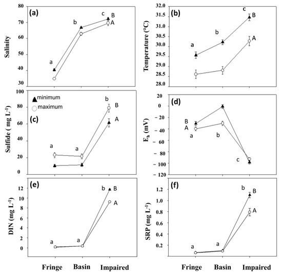
Figure 5.
Temporal variability of (a) salinity, (b) temperature, (c) sulfides, (d) Eh, (e) dissolved inorganic nitrogen (DIN), and (f) soluble reactive phosphorus (SRP) at the minimum and maximum flooding seasons for the three study sites. The different lower-case letters represent the significant differences between sites. The different upper-case letters indicate significant seasonal differences (minimum and maximum flooding).
3.3.3. Soil
There were significant differences between depths in soil bulk density (K-W test, χ2 = 20.5, p < 0.0001), with the lowest values (0.22 ± 0.008 g cm−3) at the surface (0–10 cm) compared to the highest values (0.40 ± 0.03 g cm−3) in the 20–30 cm horizon (Figure S1). There were no significant differences between sites in the superficial depth (0–10 cm, 0.22 ± 0.2 g cm−3). At the 10–20 cm depth, the bulk density was highest in the basin site (0.34 ± 0.33 g cm−3). Finally, the bulk density was higher in the basin and impaired sites than in the fringe site (0.35 ± 0.02 g cm−3 vs. 0.44 ± 0.2 g cm−3; Figure S1).
There were also significant differences in the organic matter between depths (K-W test, χ2 = 25.7, p = 0.048). Organic matter was higher in the impaired and basin sites than in the fringe site (Figure S1). However, this trend was opposite in the deeper depth (20–30 cm), with lower values in the basin and impaired sites (8.13 ± 1.86) compared to the fringe site (12 ± 3%; Figure S1).
3.4. Microtopography Transect
An apparent microtopographic variation was observed on each site, influencing the level and length of the flooding on each site directly. Specifically, the topographic relief was reduced from the basin (0.126 msnm) to the impaired site (−0.106 msnm; Figure S2). In addition, signs of degradation were observed with defoliated trees and some dead in the microtopographic height below 0.09 masl. From 180 m of inland distance, the microtopographic height was less than 0.069 masl; in this place only, dead trees and waterlogging were recorded. This section may be divided into subheadings. It should provide a concise and precise description of the experimental results, their interpretation, as well as the experimental conclusions that can be drawn.
3.5. Relationship between Biogeochemical Variables and Flooding Period
According to the GLM, the effect of the flooding on the sulfide concentration was significant in the three sites (Table 2). Additionally, there was a positive correlation between the sulfide concentration and the flooding period (fringe r2 = 0.85, p = 0.0001; basin r2 = 0.55, p < 0.0001; impaired r2 = 0.82, p = 0.0001; Figure 6). After 120 days of flooding at the impaired site, the sulfide concentration was higher (91.2 ± 10.7 mg L−1, December 2017). In contrast, the sulfide concentration was lower (3.2 ± 0.83 mg L−1) in the preserved basin site after ten days of flooding (3.2 ± 0.83 mg L−1, July 2016).
Table 2.
The effect of the flooding time over sulfide concentrations in the fringe, basin, and impaired mangrove forests.

Figure 6.
The linear relationship between the sulfide concentration and the flooding period in each mangrove study site. (a) Fringe mangrove, (b) basin mangrove, and (c) impaired site.
The GLM between flooding time and the other environmental variables (temperature, salinity, pH, Eh, DIN, SRP) was significant. Salinity was significant for the fringe site (r2 = −0.65; p = 0.0111), temperature (r2 = −0.71; p = 0.0043), and the Eh (r2 = −0.65; p = 0.0113). Temperature was significant for the basin site (r2 = −0.86; p < 0.0001). DIN (r2 = −0.61; p = 0.0161) and temperature (r2 = −0.50; p = 0.0003) were significant correlations for the impaired site.
4. Discussion
The absence of vegetation on the impaired site was related by the alteration of the hydroperiod pattern, high sulfide concentration, and low redox potential of soil. Prolonged soil water saturation at the impaired site reduced oxygen availability, favoring environmental reduced conditions and the increase of sulfides concentration, which are critical stressors for vegetation [3,15,45]. The strong correlation of flooding time with sulfide concentration on the impaired site highlighted the negative effect of this regulator on vegetation. In contrast, the sulfide concentration was lower in the sites with established vegetation and higher redox potential. Such a condition is related to high oxygen intake towards the soil by the pneumatophores and the mangroves’ supporting roots [16,46,47,48,49].
There was a higher frequency but shorter flooding time in the fringe, representing the natural hydroperiod for native vegetation in a site close to the main water body. The tide pattern produced variations of up to 35 cm of flooding per day and higher flood frequency, allowing water entry and exit to the wetland. This behavior favored that the regulators such as salinity, temperature, and sulfide concentration were not very high. An inverse pattern occurred in the basin and the impaired sites, as the more distant sites may have less hydrological connectivity, reduced water movement, and longer flooding times. This increased sulfide concentration, salinity, and temperature [26,50], which would result from a reduced or blocked hydrological connectivity between the different basin sites on estuaries such as in Estero Pargo.
Nutrients (DIN, SRP) gradually increased from the fringe and basin sites towards the impaired site, probably due to the impaired site’s loss of connectivity, erosion, and soil compaction. The absence of a tidal regime and lower soil surface level prevented the exit of the water and organic and inorganic compounds. Stagnation and evaporation increase the concentration of soil nutrients. The waterlogging and the decrease in topography from the basin towards the impaired site favor soil anaerobic conditions, increasing the concentration of reduced compounds such as sulfides, ammonium, and methane [49,51,52,53,54,55,56,57]. The increase in organic matter and low soil density result from the loss of connectivity between the impaired site and the main tidal channel of Estero Pargo.
Additionally, organic matter in the superficial depth of the impaired site may indicate that litter cannot be drained due to a lack of connectivity to the tidal creeks. Such determination resulted from the slow decomposition typical of anoxic soils [55,58,59]. The lower bulk density in the superficial soil depth was related to soil degradation in wetlands, which was primarily due to waterlogging [60,61]. Furthermore, the microtopographic gradient at the impaired site indicates that the collapse of organic soils caused the loss in elevation; the degradation and loss of the mangrove roots and associated soil were the primary sources for soil formation in mangroves [62,63]. Mangrove basins (A. germinans) are more vulnerable to submergence from sea-level rise [64].
Furthermore, anoxia, high organic matter, and a high denitrification rate deplete the nitrite and nitrate reserves and increase ammonia, which is toxic for plants even in low concentrations [58,59,65]. The lack of vegetation suggests that nutrients at the impaired site cannot be recycled or used, contributing to eutrophication [66,67]. Although N and P are limiting factors for vegetation [58], we found no evidence that mangrove degradation was associated with high nutrient concentrations. Therefore, massive tree mortality must be due to regulators such as high concentration of sulfides and alterations of the hydroperiod. There was no natural regeneration because the affected regulators (i.e., sulfides) and relief loss precluded the propagules’ establishment and growth. Finally, the lack of vegetation, especially A. germinans trees at the impaired site, cannot be solely attributed to salinity. Some black mangrove forests can grow and reproduce without damaging their structure in salinities up to 80 [61,68,69].
This study observed the effect of the maximum and minimum flooding seasons over the biogeochemical conditions. The increase in salinity during the minimum flooding season was due to a reduced water flow (lack of rainfall and surface water). Moreover, sun radiation is relatively high, increasing temperature, water evaporation, and salinity [13]. A decline in tree density at the fringe and basin sites has been reported [50]. Nevertheless, A. germinans increased its dominance on both sites except in the impaired area [70]. These changes result from hydrology-related variations in the biogeochemical conditions.
The hydroperiod and relatively low salinity determine the richness and species distribution on the study sites. Furthermore, the time and level of flooding on each site determined the distribution and density of species, reflecting their tolerance to flooding. For example, A. germinans and L. racemosa develop on shallow flooding sites, and R. mangle is established on prolonged flooded sites such as the fringe if there is a functional connection [3,30,71]. Contrariwise, monospecific A. germinans mangroves develop in the basin under relatively higher salinity [72,73,74,75]. The decline of interstitial salinity could be due to an increase in the frequency of flooding. Our records from 1994 to 2002 document a mean decrease of 11%: the average salinity was 45 at the fringe site and 70 at the basin site [26]. In this study, the mean salinity in the fringe site was 37.9 and 65.1 in the basin. The interstitial salinity decrease resulted from the greater flooding frequency due to the restoration actions [13]. Our results show that sulfides, a critical regulator, also decrease.
5. Conclusions
- The most critical regulator besides salinity in tidal-dominated mangroves was the sulfides, with the highest concentrations occurring at the end of the peak flood season.
- The maximum flooding season was from September to January, and the minimum flooding season was from February to August for Laguna de Terminos.
- In this context, the fringe mangroves are connected to the central water bodies. In contrast, the black mangrove predominates in inner basin sites, which are more fragile because they depend on the superficial flow and are distant to the primary water sources.
- The interruption of water flow will cause tree death and soil deterioration as regulators such as lower redox potential, lower sulfide concentration, and high salinity become critical with prolonged flooding and evaporation.
- Increased hydrological connectivity through the hydrological restoration of areas affected by soil salinity and sulfides can contribute to the natural establishment and growth of mangroves. Our results can support decisions on mangrove management or restoration strategies.
Supplementary Materials
The following supporting information can be downloaded at: https://www.mdpi.com/article/10.3390/f13081307/s1, Figure S1: Soil bulk density and organic matter in three depths in the fringe, basin, and impaired sites. Depth of soil depths are: 0–10 cm, diamonds; 10–20 cm; triangles, 20–30 cm. Vertical bars indicate one SE. Figure S2: Topography along a 160 m long transect from the fringe to the impaired site at Estero Pargo. The water level corresponds to the beginning of the maximum flooding season in September 2016.
Author Contributions
Conceptualization: R.P.-C. and A.Z.-J. Formal analysis: R.P.-C., S.M.-S., J.C.-D. and A.Z.-J. Investigation: R.P.-C., S.M.-S. and A.Z.-J. Methodology: R.P.-C., A.Z.-J., S.M.-S., J.C.-D. and M.M.-I. Software: R.P.-C., J.C.-D. and S.M.-S. Supervision: R.P.-C., A.Z.-J., J.L.-P. and M.M.-I. Writing—original draft: R.P.-C., S.M.-S., A.Z.-J., J.C.-D., O.C.-H. and J.O.-G. Writing—review and editing: J.L.-P., M.M.-I. and A.L.L.-D. All authors have read and agreed to the published version of the manuscript.
Funding
This research received no external funding.
Data Availability Statement
Not applicable.
Acknowledgments
We thank Herminia Rejón Salazar and the ‘Community of Mangrove Restorers’ from Isla Aguada for their support with the field work; Josefina Santos Ramírez, Tomás Zaldívar Jiménez, Mario Alejandro Gómez Ponce, Hernán Álvarez Guillén, and Andrés Reda Deara for their assistance with logistics and field data collection; and Fermín S. Castillo-Sandoval for lab analysis. We would also like to thank José Hernández Nava from CONANP-Laguna de Términos for the facilities to carry out our surveys.
Conflicts of Interest
The authors declare no conflict of interest.
References
- Hayden, H.L.; Granek, E.F. Coastal sediment elevation change following anthropogenic mangrove clearing. Estuar. Coast. Shelf Sci. 2015, 165, 70–74. [Google Scholar] [CrossRef]
- McKee, K.L. Soil Physicochemical Patterns and Mangrove Species Distribution—Reciprocal Effects? J. Ecol. 1993, 81, 477. [Google Scholar] [CrossRef]
- Twilley, R.R.; Rivera-Monroy, V.H. Developing performance measures of mangrove wetlands using simulation models of hydrology, nutrient biogeochemistry, and community dynamics. J. Coast. Res. 2005, 21, 79–93. [Google Scholar] [CrossRef]
- Krauss, K.W.; Doyle, T.W.; Twilley, R.R.; Rivera-Monroy, V.H.; Sullivan, J.K. Evaluating the relative contributions of hydroperiod and soil fertility on growth of south Florida mangroves. Hydrobiologia 2006, 569, 311–324. [Google Scholar] [CrossRef]
- Lee, S.Y.; Primavera, J.H.; Dahdouh-Guebas, F.; Mckee, K.; Bosire, J.O.; Cannicci, S.; Diele, K.; Fromard, F.; Koedam, N.; Marchand, C.; et al. Ecological role and services of tropical mangrove ecosystems: A reassessment. Glob. Ecol. Biogeogr. 2014, 23, 726–743. [Google Scholar] [CrossRef]
- Pérez-Ceballos, R.; Zaldívar-Jiménez, A.; Canales-Delgadillo, J.; López-Adame, H.; López-Portillo, J.; Merino-Ibarra, M. Determining hydrological flow paths to enhance restoration in impaired mangrove wetlands. PLoS ONE 2020, 15, e0227665. [Google Scholar] [CrossRef]
- Alongi, D.M. Present state and future of the worlds mangrove forests. Environ. Conserv. 2002, 29, 331–349. [Google Scholar] [CrossRef]
- Fiedler, S.; Vepraskas, M.J.; Richardson, J.L. Soil Redox Potential: Importance, Field Measurements, and Observations. Adv. Agron. 2007, 94, 1–54. [Google Scholar] [CrossRef]
- Fink, D.F.; Mitsch, W.J. Hydrology and nutrient biogeochemistry in a created river diversion oxbow wetland. Ecol. Eng. 2007, 30, 93–102. [Google Scholar] [CrossRef]
- Schoeneberger, P.J.; Wysocki, D.A. Hydrology of soils and deep regolith: A nexus between soil geography, ecosystems and land management. Geoderma 2005, 126, 117–128. [Google Scholar] [CrossRef]
- Agraz-Hernández, C.M.; Osti-Sáenz, J.; Chan-Keb, C.A.; Chan-Canul, E.; Gómez-Ramírez, D.; Requena-Pavón, G.; Reyes-Castellanos, J. Programa Regional para la Caracterización y el Monitoreo de Ecosistemas de Manglar del Golfo de México y Caribe Mexicano: Campeche. Universidad Autónoma Campeche. Centro de Ecología Pesquería y Oceanografía del Golfo de México. Informe final SNIB-CONABIO. Proyecto FN010, D.F. México. 2012. Available online: http://www.conabio.gob.mx/institucion/proyectos/resultados/InfFN010.pdf (accessed on 12 August 2022).
- Chen, R.; Twilley, R.R. A gap dynamic model of mangrove forest development along gradients of soil salinity and nutrient resources. J. Ecol. 1998, 86, 37–51. [Google Scholar] [CrossRef]
- Echeverría-Ávila, S.; Pérez-Ceballos, R.; Zaldívar-Jiménez, A.; Canales-Delgadillo, J.; Brito-Pérez, R.; Merino-Ibarra, M.; Vovides, A. Regeneración natural de sitios de manglar degradado en respuesta a la restauración hidrológica. Madera y Bosques 2019, 25, e2511754. [Google Scholar] [CrossRef]
- Osland, M.J.; Day, R.H.; Hall, C.T.; Feher, L.C.; Armitage, A.R.; Cebrian, J.; Dunton, K.H.; Hughes, A.R.; Kaplan, D.A.; Langston, A.K.; et al. Temperature thresholds for black mangrove (Avicennia germinans) freeze damage, mortality and recovery in North America: Refining tipping points for range expansion in a warming climate. J. Ecol. 2019, 108, 654–665. [Google Scholar] [CrossRef]
- Lamers, L.P.M.; Govers, L.L.; Janssen, I.C.J.M.; Geurts, J.J.M.; Van der Welle, M.E.W.; Van Katwijk, M.M.; Van der Heide, T.; Roelofs, J.G.M.; Smolders, A.J.P. Sulfide as a soil phytotoxin—A review. Front. Plant Sci. 2013, 4, 268. [Google Scholar] [CrossRef] [PubMed]
- McKee, K.L.; Mendelssohn, I.A.; Hester, M.W. Reexamination of Pore Water Sulfide Concentrations and Redox Potentials Near the Aerial Roots of Rhizophora mangle and Avicennia germinans. Am. J. Bot. 1988, 75, 1352. [Google Scholar] [CrossRef]
- Valiela, I.; Bowen, J.L.; York, J.K. Mangrove Forests: One of the World’s Threatened Major Tropical Environments. Bioscience 2001, 51, 807. [Google Scholar] [CrossRef]
- Goldberg, L.; Lagomasino, D.; Thomas, N.; Fatoyinbo, T. Global declines in human-driven mangrove loss. Glob. Chang. Biol. 2020, 26, 5844–5855. [Google Scholar] [CrossRef]
- Valderrama-Landeros, L.H.; Rodríguez-Zúñiga, M.T.; Troche-Souza, C.; Velázquez-Salazar, S.; Villeda-Chávez, E.; Alcántara-Maya, J.A.; Vázquez-Balderas, B.I.; Cruz-López, M.I.; Ressl, R. Manglares de México: Actualización y Exploración de los Datos del Sistema de Monitoreo 1970/1980–2015, 1st ed.; Comisión Nacional para el Conocimiento y Uso de la Biodiversidad: Ciudad de México, Mexico, 2017; p. 128. [Google Scholar]
- López-Portillo, J.; Zaldívar-Jiménez, A.; Lara-Domínguez, A.N.; Pérez-Ceballos, R.; Bravo-Mendoza, M.; Núñez-Álvarez, N.; Aguirre-Franco, L. Hydrological Rehabilitation and Sediment Elevation as Strategies to Restore Mangroves in Terrigenous and Calcareous Environments in Mexico. In Wetland Carbon and Environmental Management, 1st ed.; Krauss, K.W., Zhu, Z., Stagg, C.L., Eds.; Wiley Online Library: Hoboken, NJ, USA, 2021; pp. 173–190. [Google Scholar]
- Canales-Delgadillo, J.; Perez-Ceballos, R.; Merino-Ibarra, M.; Cardoza-Cota, G.; Cardoso-Mohedano, J.G. The effect of mangrove restoration on avian assemblages of a coastal lagoon in southern Mexico. PeerJ 2019, 7, e7493. [Google Scholar] [CrossRef]
- Villalobos-Zapata, G.J.; Yáñez-Arancibia, A.; Day, J.W., Jr.; Lara-Domínguez, A. Ecología y manejo de los manglares en la Laguna de Términos, Campeche, México. In Ecosistemas de Manglar en América Tropical; Yáñez-Arancibia, A., Lara-Domínguez, A.L., Eds.; Instituto de Ecología A.C.: Xalapa, Mexico; UICN/ORMA: San José, Costa Rica; NOAA/NMFS: Silver Spring, MO, USA, 1999; pp. 263–274. [Google Scholar]
- Arriaga, L.; Espinoza, J.M.; Aguilar, C.; Martínez, E.; Gómez, L.; Loa, E. Regiones terrestres prioritarias de México. Escala de trabajo 1:1,000,000; Comisión Nacional para el Conocimiento y uso de la Biodiversidad: Mexico City, Mexico, 2000; p. 611. [Google Scholar]
- Yáñez-Arancibia, A.; Day, J.W., Jr. Ecological characterization of Terminos Lagoon, a tropical lagoon-estuarine system in the southern Gulf of Mexico. Oceanol. Acta 1982, 5, 431–440. [Google Scholar]
- Instituto Nacional de Ecología. Programa de Manejo del Área de Protección de Flora y Fauna Laguna de Términos; INE-SEMARNAP: Mexico City, Mexico, 1997; p. 166. [Google Scholar]
- Coronado-Molina, C.A.; Alvarez-Guillen, H.; Day, J.W.; Reyes, E.; Perez, B.C.; Vera-Herrera, F.; Twilley, R. Litterfall dynamics and nutrient cycling in mangrove forest of Southern Everglades, Florida and Terminos Lagoon, Mexico. Wetl. Ecol. Manag. 2000, 20, 123–136. [Google Scholar] [CrossRef]
- Escudero, M.; Silva, R.; Mendoza, E. Beach erosion driven by natural and human activity at Isla del Carmen Barrier Island, Mexico. J. Coast. Res. 2014, 71, 62–74. [Google Scholar] [CrossRef]
- Rivera-Monroy, V.H.; Madden, C.J.; Day, J.W.; Twilley, R.R.; Vera-Herrera, F.; Alvarez-Guillén, H. Seasonal coupling of a tropical mangrove forest and an estuarine water column: Enhancement of aquatic primary productivity. Hydrobiologia 1998, 379, 41–53. [Google Scholar] [CrossRef]
- Feller, I.C.; McKee, K.L.; Whigham, D.F.; O’Neill, J.P. Nitrogen vs. phosphorus limitation across an ecotonal gradient in a mangrove forest. Biogeochemistry 2003, 62, 145–175. [Google Scholar] [CrossRef]
- Pool, D.J.; Snedaker, S.; Lugo, A. Structure of mangrove forests in Florida, Puerto Rico, Mexico, and Costa Rica. Biotropica 1977, 9, 195–212. [Google Scholar] [CrossRef]
- Snedaker, S.C.; Snedaker, J.G. The Mangrove Ecosystem: Research Methods; Unesco: Bungay, UK, 1984; p. 251. [Google Scholar]
- Valdez-Hernández, J.I. Aprovechamiento Forestal de manglares en el estado de Nayarit costa Pacifica de México. Madera Y Bosques 2002, 8, 129–145. [Google Scholar] [CrossRef][Green Version]
- Cleveland, W.S. Robust locally weighted regression and smoothing scatterplots. J. Am. Stat. Assoc. 1979, 74, 829–836. [Google Scholar] [CrossRef]
- Rodríguez-Zúñiga, M.T.; Pérez-Ceballos, R.; Zaldívar-Jiménez, A.; Lara-Domínguez, A.; Teutli-Hernández, C.; Herrera-Silveira, J. Muestreo de variables hidrológicas, fisicoquímicas y del sedimento. In Métodos para la caracterización de los manglares mexicanos: Un enfoque espacial multi-escala; Rodríguez Zúñiga, M.T., Villeda-Chávez, E., Vázquez-Lule, A.D., Bejarano, M., Cruz-López, M.I., Olguín, M., Villela-Gaytán, S.A., Flores, R., Eds.; Comisión Nacional para el Conocimiento y Uso de la Biodiversidad: Ciudad de México, Mexico, 2018; pp. 131–169. [Google Scholar]
- Grasshoff, K.; Kremling, K.; Ehrhardt, M. Methods of Seawater Analysis, 3rd ed.; WILEY-VCH Verlag GmbH: Mexico City, Mexico, 1999. [Google Scholar] [CrossRef]
- Kirkwood, D. Sanplus Segmented Flow Analyzer and Its Applications. Seawater Analysis; Skalar: Amsterdam, The Netherlands, 1994. [Google Scholar]
- Rabenhorst, M.C.; Hively, W.D.; James, B.R. Measurements of Soil Redox Potential. Soil Sci. Soc. Am. J. 2009, 73, 668–674. [Google Scholar] [CrossRef]
- Chen, R.; Twilley, R.R. Patterns of Mangrove Forest Structure and Soil Nutrient Dynamics Along the Shark River Estuary, Florida. Estuaries 1999, 22, 955–970. [Google Scholar] [CrossRef]
- Castañeda-Moya, E.; Twilley, R.R.; Rivera-Monroy, V.H. Allocation of biomass and net primary productivity of mangrove forests along environmental gradients in the Florida Coastal Everglades, USA. For. Ecol. Manag. 2013, 307, 226–241. [Google Scholar] [CrossRef]
- Konare, H.S.; Yost, R.M.; Doumbia, W.; McCarty, G.; Jarju, A.; Kablan, R. Loss on ignition: Measuring soil organic carbon in soils of the Sahel, West Africa. Afr. J. Agric. Res. 2010, 5, 3088–3095. [Google Scholar]
- Pérez-Ceballos, R.; Echeverría-Ávila, S.; Zaldívar-Jiménez, A.; Zaldívar-Jiménez, T.; Herrera-Silveira, J. Contribution of microtopography and hydroperiod to the natural regeneration of Avicennia germinans in a restored mangrove forest. Ciencias Mar. 2017, 43, 55–67. [Google Scholar] [CrossRef]
- Tukey, J.W. Exploratory Data Analysis; Addison-Wesley Pub. Co.: Reading, MA, USA, 1977. [Google Scholar]
- Di Rienzo, J.; Balzarini, M.; Robledo, C.; Casanoves, F.; Gonzales, L.; Tablada, E. InfoStat Software Estadístico; FCA Universidad Nacional de Córdoba: Córdoba, Argentina, 2018. [Google Scholar]
- R Core Team. R: A Language and Environment for Statistical Computing; R Foundation for Statistical Computing: Vienna, Austria, 2013; p. 3. Available online: https://www.R-project.org/ (accessed on 12 August 2022).
- Nickerson, N.H.; Thibodeau, F.R. Association between pore water sulfide concentrations and the distribution of mangroves. Biogeochemistry 1985, 1, 183–192. [Google Scholar] [CrossRef]
- Marchand, C.; Lallier-Vergès, E.; Baltzer, F. The composition of sedimentary organic matter in relation to the dynamic features of a mangrove-fringed coast in French Guiana. Estuar. Coast. Shelf Sci. 2003, 56, 119–130. [Google Scholar] [CrossRef]
- Lyimo, T.L.; Mushi, D. Sulfide Concentration and Redox Potential Patterns in Mangrove Forests of Dar es Salaam: Effects on Avicennia marina and Rhizophora mucronata Seedling Establishment. West. Indian Ocean J. Mar. Sci. 2007, 4, 163–174. [Google Scholar] [CrossRef]
- Coull, B.C. Role of meiofauna in estuarine soft-bottom habitats. Aust. J. Ecol. 1999, 24, 327–343. [Google Scholar] [CrossRef]
- Reef, R.; Feller, I.C.; Lovelock, C.E. Nutrition of mangroves. Tree Physiol. 2010, 30, 1148–1160. [Google Scholar] [CrossRef]
- Day, J.W., Jr.; Coronado-Molina, C.; Vera-Herrera, F.R.; Twilley, R.R.; Rivera-Monroy, V.H.; Alvarez-Guillen, H.; Day, R.; Conner, W. A 7 year record of above-ground net primary production in a southeastern Mexican mangrove forest. Aquat. Bot. 1996, 55, 39–60. [Google Scholar] [CrossRef]
- Poret, N.; Twilley, R.R.; Rivera-Monroy, V.H.; Coronado-Molina, C. Belowground decomposition of mangrove roots in Florida coastal everglades. Estuaries Coasts 2007, 30, 491–496. [Google Scholar] [CrossRef]
- Santos-Ramirez, J. Efecto de las Condiciones Ambientales Sobre la Descomposición de Raíces del Mangle Avicennia germinans en Sitios Con Restauración de Isla del Carmen, Campeche. Master’s Thesis, Universidad Autónoma del Carmen, Ciudad del Carmen, Campeche, Mexico, 24 November 2017. [Google Scholar]
- Moreno-Casasola, P.; Warner, B. Breviario Para Describir, Observar Y Manejar Humedales, 3rd ed.; Serie Costa Sustentable no 1; RAMSAR, Instituto de Ecología, A.C., CONANP, US Fish and Wildlife Service, US State Department: Xalapa, Mexico, 2009; p. 406. [Google Scholar]
- Cruz-Lucas, M.A. Topografía y Factores Ambientales Relacionados a las Comunidades Vegetales en un Humedal. Master’s Thesis, Universidad Veracruzana, Veracruz, Mexico, 27 October 2010. [Google Scholar]
- Ramírez-Barrón, E. Distribución de las especies de manglar en relación a la microtopografía y la manipulación experimental del hidroperiodo para abatir la salinidad intersticial en una marisma hipersalina, en el estero de Urías: Mazatlán Sinaloa. Master´s Thesis, Universidad Nacional Autónoma de México, Ciudad de México, Mexico, August 2014. [Google Scholar]
- Flores-Verdugo, F.; Moreno-Casasola, P.; Agraz-Hernández, M.; López-Rosas, H.; Benitez-Pardo, D. La topografía y el hidroperíodo: Dos factores que condicionan la restauración de los humedales costeros. Boletín La Soc. Botánica México 2007, 80, 33–47. [Google Scholar] [CrossRef]
- Agraz-Hernández, C.M.; del Río-Rodríguez, R.E.; Chan-Keb, C.A.; Osti-Saenz, J.; Muñiz-Salazar, R. Nutrient removal efficiency of Rhizophora mangle (L.) seedlings exposed to experimental dumping of municipal waters. Diversity 2018, 10, 16. [Google Scholar] [CrossRef]
- Alongi, D.M. Early growth responses of mangroves to different rates of nitrogen and phosphorus supply. J. Exp. Mar. Bio. Ecol. 2011, 397, 85–93. [Google Scholar] [CrossRef]
- Alongi, D.M.; Wattayakorn, G.; Boyle, S.; Tirendi, F.; Payn, C.; Dixon, P. Influence of roots and climate on mineral and trace element storage and flux in tropical mangrove soils. Biogeochemistry 2004, 69, 105–123. [Google Scholar] [CrossRef]
- Krauss, K.W.; Demopoulos, A.W.J.; Cormier, N.; From, A.S.; McClain-Counts, J.P.; Lewis, R.R. Ghost forests of Marco Island: Mangrove mortality driven by belowground soil structural shifts during tidal hydrologic alteration. Estuar. Coast. Shelf Sci. 2018, 212, 51–62. [Google Scholar] [CrossRef]
- Flores Verdugo, F.J.; Agraz Hernández, C.; Benítez Pardo, D. Ecosistemas acuáticos costeros: Importancia, retos y prioridades para su conservación. In Perspectivas Sobre Conservación de Ecosistemas Acuáticos en México, 1st ed.; Sánchez, O., Herzig, M., Peters, E., Márque-Huitzil, R., Zambrano, L., Eds.; Secretaría de Medio Ambiente y Recursos Naturales Instituto Nacional de Ecología U.S. Fish & Wildlife Service Unidos para la Conservación, A.C.; Universidad Michoacana de San Nicolás Hidalgo: Morelia, Mexico, 2007; pp. 147–166. Available online: https://docplayer.es/12780089-Ecosistemas-acuaticos-costeros-importancia-retos-y-prioridades-para-su-conservacion.html (accessed on 13 June 2022).
- Reddy, K.R.; De Laune, R.D. Biogeochemistry of Wetlands, 1st ed.; CRC Press: Boca Raton, FL, USA, 2008; p. 800. [Google Scholar]
- Flores-Verdugo, F.J.; Agraz-Hernández, C.M.; Benítez-Pardo, D. Creación y Restauración de Ecosistemas de Manglar: Principios Básicos. In Manejo Costero Integral: El Enfoque Municipal; Moreno-Casasola, P., Peresbarbosa, E., Travieso, A.C., Eds.; Instituto de Ecología: Xalapa, Mexico, 2005; pp. 1093–1110. [Google Scholar]
- Krauss, K.W.; Mckee, K.L.; Lovelock, C.E.; Cahoon, D.R.; Saintilan, N.; Reef, R.; Chen, L. How mangrove forests adjust to rising sea level. New Phytol. 2013, 202, 19–34. [Google Scholar] [CrossRef]
- Kristensen, E.; Alongi, D.M. Control by fiddler crabs (Uca vocans) and plant roots (Avicennia marina) on carbon, iron, and sulfur biogeochemistry in mangrove sediment. Limnol. Oceanogr. 2006, 51, 1557–1571. [Google Scholar] [CrossRef]
- Komiyama, A.; Ong, J.E.; Poungparn, S. Allometry, biomass, and productivity of mangrove forests: A review. Aquat. Bot. 2008, 89, 128–137. [Google Scholar] [CrossRef]
- Jiang, G.F.; Goodale, U.M.; Liu, Y.Y.; Hao, G.Y.; Cao, K.F. Salt management strategy defines the stem and leaf hydraulic characteristics of six mangrove tree species. Tree Physiol. 2017, 37, 389–401. [Google Scholar] [CrossRef] [PubMed]
- Feller, I.C.; Lovelock, C.E.; McKee, K.L. Nutrient addition differentially affects ecological processes of Avicennia germinans in nitrogen versus phosphorus limited mangrove ecosystems. Ecosystems 2007, 10, 347–359. [Google Scholar] [CrossRef]
- Valderrama, L.; Troche, C.; Rodriguez, M.T.; Marquez, D.; Vázquez, B.; Velázquez, S.; Vázquez, A.; Cruz, M.I.; Ressi, R. Evaluation of mangrove cover changes in Mexico during the 1970-2005 Period. Wetlands 2014, 34, 747–758. [Google Scholar] [CrossRef]
- Day, J.J.; Conner, W.; Ley-Lou, F.; Day, R.H.; Navarro, A.M. The Productivity and Composition of Mangrove Forest, Laguna De Terminos, Mexico. Aquat. Bot. 1987, 27, 267–284. [Google Scholar] [CrossRef]
- Cardona-Olarte, P.; Twilley, R.R.; Krauss, K.W.; Rivera-Monroy, V. Responses of neotropical mangrove seedlings grown in monoculture and mixed culture under treatments of hydroperiod and salinity. Hydrobiologia 2006, 569, 325–341. [Google Scholar] [CrossRef]
- Pérez-Castillo, V.F. Dinámica de C, N, P y Fe en Agua y Sedimentos en el Humedal Natural Ciénega de Tamasopo, S.L.P. Ph.D. Thesis, Facultad de Ciencias Químicas, Ingeniería y Medicina, Programas Multidisciplinarios de Posgrado en Ciencias Ambientales, Universidad Autónoma de San Luis Potosí, San Luis Potosí, Mexico, 2018. [Google Scholar]
- Jiménez, J.A.; Sauter, K. Structure and Dynamics of Mangrove Forests Along a Flooding Gradient. Estuaries 1991, 14, 49–56. [Google Scholar] [CrossRef]
- Yáñez–Espinosa, L.; Angeles, G.; López-Portillo, J.; Bárrales, S. Variación anatómica de la madera de Avicennia germinans en la laguna de la mancha, Veracruz, México. Boletín la Soc. Botánica México 2009, 15, 7–15. [Google Scholar] [CrossRef]
- Da-Cruz, C.C.; Mendoza, U.N.; Queiroz, J.B.; Da-Costa, N.; Lara, R.J. Distribution of mangrove vegetation along inundation, phosphorus, and salinity gradients on the Bragança Peninsula in Northern Brazil. Plant Soil 2013, 370, 393–406. [Google Scholar] [CrossRef]


Publisher’s Note: MDPI stays neutral with regard to jurisdictional claims in published maps and institutional affiliations. |
© 2022 by the authors. Licensee MDPI, Basel, Switzerland. This article is an open access article distributed under the terms and conditions of the Creative Commons Attribution (CC BY) license (https://creativecommons.org/licenses/by/4.0/).