Abstract
Sustainable forest management requires accurate biometric tools to estimate forest site quality. This is particularly relevant for prescribing adequate silvicultural treatments of forest management planning. The aim of this research was to incorporate topographic and climatic variables into dominant height growth models of patula pine stands to improve the estimation of forest stand productivity. Three generalized algebraic difference approach (GADA) models were fit to a dataset from 66 permanent sampling plots, with six re-measurements and 77 temporary inventory sampling plots established on forest stands of patula pine. The nested iterative approach was used to fit the GADA models, and goodness-of-fit statistics such as the root mean square error, Akaike’s Information Criterion, and Bias were used to assess their performance. A Hossfeld IV GADA equation type that includes altitude, slope percentage, mean annual precipitation, and mean annual minimum temperature produced the best fit and estimation. Forest site productivity was negatively affected by altitude, while increasing the mean annual minimum temperature suggested the fastest-growing rates for dominant tree height.
1. Introduction
The estimation of forest site productivity is a key element in sustainable forest management planning [1,2]; its accurate assessment allows the quantification of stand capacity for the production of raw materials, and the planning of silvicultural treatments throughout forest rotation [3].
The most commonly used approach for assessing a stand’s productivity is site index (SI), which is based on modeling the existing height–age relationship of the dominant and co-dominant trees present in the stand [4,5]. This is relevant because SI provides key information for the construction of one of the most important tools for forest management planning [6]: the well-known forest growth and yield systems [7,8,9].
Stand productivity depends directly on the inherent characteristics of the site, such as soil type, temperature, solar radiation, altitude, climatic variables, etc., as well as those characteristics that affect its growth and yield [10,11,12,13]. Previous studies have reported better forest site productivity classification when the models include climatic and topographic variables to determine the factors that affect tree development [14,15,16,17].
The addition of climate variables to SI models and forest growth and yield systems could make them climate-sensitive, which has enormous value in helping with the prediction of forest site productivity under probable future scenarios of climate change [18]. SI could even be considered a predictor of the effect of climate change on forest growth [19,20,21]. These types of models could also help forest managers to adapt silvicultural treatments of managed stands [22].
In forests of Southern Mexico, several studies on dominant height growth and SI have been developed for patula pine (Pinus patula Schiede ex Schltdl. and Cham.) using the algebraic difference approaches (ADA) [23] and its generalized version (GADA) [24]. Santiago-García et al. [25] reported good results with a polymorphic Levakovic II ADA equation to estimate the SI for patula pine. On a broader scale of analysis, Castillo-López et al. [26] fitted a Chapman-Richards GADA model using stem analysis data from dominant trees to estimate the SI in the Northern Sierra of Oaxaca, Mexico, with good results. Recently, Nava-Nava et al. [27] fit dominant height growth models for patula pine, where ADA and GADA models based on a Chapman-Richards equation were used. However, none have incorporated the effects of climatic and topographical variables into the model fitting process.
The objective of this research was to fit dominant height growth equations with the addition of topographic and climatic variables for naturally regenerated patula pine stands located in the Sierra Juárez, Oaxaca, in Southern Mexico. The hypothesis was that adding topographic and climate variables to the GADA models would improve the accuracy of estimations of forest site productivity through SI estimation.
2. Materials and Methods
2.1. Study Area
The study was conducted in the communal forest of Ixtlán de Juárez, Oaxaca, Mexico (Figure 1), located geographically in the coordinate range of 17°23′0.50″–17°23′0.58″ N and 96°28′45″–96°28′53″ W. The mean altitude is 2700 m. Patula pine has the highest commercial value for timber production in the region [28,29].
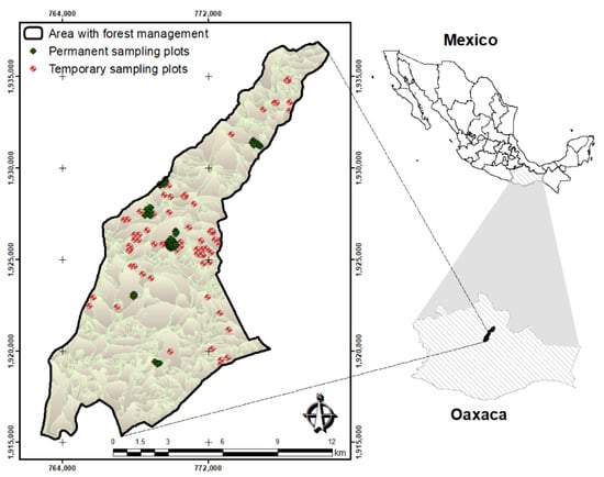
Figure 1.
Study site location and sampled plots in Ixtlán de Juárez, Oaxaca, Southern Mexico.
The most common soil groups found in the study area are acrisol, luvisol, and cambisol. The predominant climates are temperate sub-humid with summer rains, and temperate humid with summer rains. The mean annual temperature is around 20 °C, and the rainfall ranges from 800 to 1200 mm [30,31].
2.2. Data
The dataset for the analysis comes from two sources: 66 square permanent sampling plots of 400 m2, with six re-measurements taken from 2015 to 2020, and 77 circular temporary plots of 1000 m2, sampled as part of a timber inventory conducted in 2014 [31]. Before the model fitting process, it was necessary to estimate the height trajectories for the temporary plot data, such as the dominant height projected over one year, with the dynamic model proposed by Nava-Nava et al. [27]. This process allowed us to create 77 additional pairs of data. Thus, the assumption to supplement the database was based on the fact that the height of the trees cannot be known with certainty, even with conventional field measurements. So, the estimation by the previous model had a complementary role in the data’s generation [32,33,34]. This allowed having the trajectories of the temporary plots to use the fit method, which requires more than one observation per plot [35,36]. The combined datasets resulted in a robust panel data source [37] (Table 1) that allowed for a more accurate inference of model parameters, and a better ability to capture the complexity of dominant height growth behavior than a single cross-section data type [38,39,40]. The combined use of data derived from permanent and temporary sampling plots resulted in robust estimates of forest site productivity [27].

Table 1.
Descriptive statistics of the data used in fitting dynamic equations for patula pine.
The permanent sampling plots were randomly distributed in stands of patula pine at different stand ages, as well as in diverse site conditions, at an altitudinal gradient from 2360 to 2960 m [25,29] (Table 1). To determine the stand’s dominant height, the total tree height of four dominant trees in each plot was measured with a CE II-D Haglöf Sweden® electronic clinometer, according to the concept of dominant height that employs the top 100 trees—of larger diameter and height—per hectare [41,42,43]. Age in the permanent sampling plots was calculated with the year in which regeneration cutting was applied, while in the temporary sampling plots, age was obtained from tree cores from the dominant trees.
Dominant tree height and age data were used to estimate the mean height (Hd; m) and mean age (A; years) at the stand level, respectively. Additionally, topographic (altitude and slope) and climatic (PTm: mean annual precipitation, MAT: mean annual temperature, Tmax: mean annual maximum temperature, and Tmin: mean annual minimum temperature) variables were obtained with ArcGIS® 10.2 software (ESRI, Redlands, CA, USA) [44]. The topographic variables were obtained from the digital elevation model version 3.0, at a resolution of 15 m [45]. Climatic variables were extracted from the Daily Surface Weather and Climatological Summaries (DAYMET) dataset with a resolution of 1 × 1 km [46] (Table 1). Those data sources have been used in several studies with suitable results [47,48]. We selected altitude, slope, precipitation, and temperature in the estimation of forest site productivity; these last two were selected as they are the most commonly used [10,15,16,18]. The MAT, Tmax, and Tmin were tested. However, to avoid collinearity, we included only Tmin in this study because it contributed most to explaining the variability of the observed data.
2.3. Data Analysis, and Model Fitting and Validation
The fit and validation of the dynamic equations were carried out with what was described by Goulding [49], and Vanclay and Skovsgaard [50], and used by Soares et al. [51]. The database partitioning was performed randomly with the “caTools” package in R [52]; in a preliminary analysis, several datasets with different proportions were tested for fit and validation. Goodness-of-fit statistics showed that the relationship with 70% for fit and 30% for validation was the best. Three extensively known GADA models were fit to the datasets: the Chapman-Richards, Hossfeld IV, and Korf equations [53,54,55], respectively, and they have been used by Socha et al. [6] and Özçelik et al. [56]. These models were named M1, M2, and M3, respectively (Table 2).
Table 2.
Base growth equation and GADA formulations fitted to combined datasets.
To analyze the effect of the climatic and topographic variables (site variables) on the dominant height growth equation, we related them to the parameters of the GADA model (Mia: fitting without site variables and Mib: fitting with site variables). The smallest root mean square error (RMSE) (6) and parameters that, according to the level of significance, would better explain the performance of the dependent variable, were identified [57]. The GADA model parameters (βi) were reparameterized as multiple regression models with topographic variables (X1) and climatic variables (X2), as illustrated below:
where X1: topographic variable (slope and altitude); X2: climatic variable (PTm and Tmin); βij: parameter of the combination j of the parameter i.
A preliminary analysis of different combinations of topographic and climatic variables allowed us to identify the best results (the largest adjusted coefficient of determination and minimal mean error) for different βi parameters (Table 3), which was the following:
where βi: GADA model parameter (i = 1,2,3); βij: parameter of the combination j of the parameter i; PTm: mean annual precipitation; Tmin: mean annual minimum temperature.
Table 3.
GADA formulations with and without site variables fitted to the datasets.
The GADA model parameters were estimated using the nested iterative procedure proposed by Tait et al. [35]. This method states that the specified initial conditions must be identical for all measurements belonging to the same sampled plot, where the initial age can be arbitrarily selected but must be different from zero. The method estimates plot-specific parameters and assumes that there are random and measurement errors in the data, which must be modeled [53]. The fitting equation was performed with the MODEL procedure of SAS/ETS® 9.3 [36].
The best model was selected based on the following goodness-of-fit statistics: the largest adjusted coefficient of determination (R2adj) (5), the minimal root mean square error (RMSE) (6), the minimal mean error (Bias) (7), and the smallest Akaike’s Information Criterion (AIC) (8) [54,58]. Furthermore, the parameter estimates should guarantee 5% significance. Autocorrelation was evaluated with the Durbin–Watson (DW) statistic (9) [59]. For the validation process, the Bias, mean square error (MSE) (10), and efficiency index (EI) (11) were calculated [51]. Additionally, a graphical analysis of the residuals and the dominant height curve trajectories vs. data was performed [60]. To achieve homoscedasticity of variance in the distribution of the residuals and estimators of consistent parameters, we used the fitting approach suggested by Kübler et al. [61] and used by Tamarit-Urias et al. [62] of , where was a weighting factor, k was a constant with a 0.5 value, and the structure of the error variance used was expressed as . Finally, the relationship of the average dominant height to topographic and climatic variables was measured with Pearson correlation coefficients (r) [63,64].
where : observed, predicted, and mean values; n: number of observations; p: number of model parameters; : residual value of the fitted model.
3. Results
All fitted GADA equations explained around 99.3% (R2adj) of the observed variability in dominant height. Additionally, all estimated parameters were statistically significantly different from zero (p ≤ 0.05) (Table 4). Figure 2 shows the SI trajectories generated with the estimated parameters of the GADA equations (Table 4). The curves describe the dominant height growth pattern appropriately at a base age of 40 years, covering the observed data, with a sigmoidal shape and a biologically desirable trend, as stated by Kiviste et al. [4].
Table 4.
Goodness-of-fit statistics of the dynamic equations for dominant height with and without the addition of topographic and climatic variables.
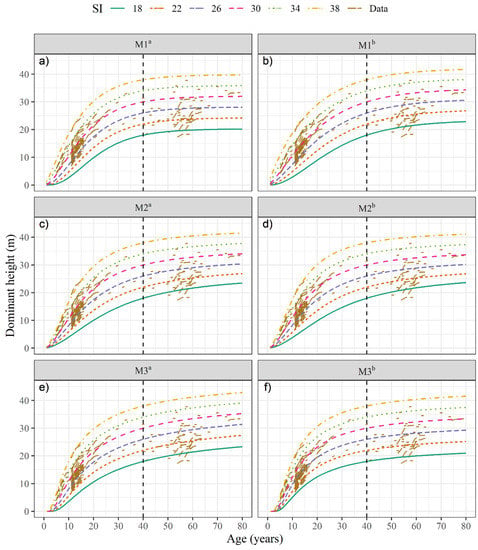
Figure 2.
Site index curves for patula pine at a base age of 40 years. M1: Chapman-Richards (a,b), M2: Hossfeld IV (c,d), M3: Korf (e,f). a Fitting without the addition of site topographic and climatic variables, and b fitting with the addition of site topographic and climatic variables.
The use of a weighting function () allowed the residuals of the equations to have a homogeneous and clustered behavior on the central reference line (zero) (Figure 3), which agrees with what Sharma and Parton [65] reported in a study with white pine (Pinus strobus L.). The values of the DW statistic suggest that the residuals are not strongly correlated (DW ≈ 2) (Table 4); otherwise, such autocorrelation could adversely affect the estimation of the standard error of the parameters [66]. The combination of time series and cross-sectional data in the fitted equations provided consistent results (Figure 3), and since the datasets were independent, it helped to reduce autocorrelation, as has been reported in other studies [27,37].
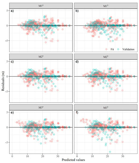
Figure 3.
Residuals of the fitted dominant-height dynamic equations for patula pine. M1: Chapman-Richards (a,b), M2: Hossfeld IV (c,d), M3: Korf (e,f). a Fitting without the addition of site topographic and climatic variables; b fitting with the addition of site topographic and climatic variables.
In the validation phase, the equations were over 95.7% effective in predicting the dominant height. The M3i equations had the highest errors (MSE and Bias) (Table 4, Figure 3e,f). The results showed that equation M1a had the highest precision and lowest bias (Table 4); however, equation M2b presents a more homogeneous distribution of the residuals (Figure 3d). The biggest gain of this equation (M2b) is the flexibility in estimating the SI under climate change scenarios and topographic conditions.
Based on the fit statistics, SI curves vs. observed data, biologically realistic trends, and the residuals plots, equation M2b (Table 4, Figure 2d and Figure 3d) is the most plausible for modeling the dominant height growth pattern of patula pine stands, and is recommended for use in the study area (Table 1). Table 5 shows the linear correlations between dominant height and topographic and climatic variables. There results indicate a high negative correlation between dominant height and altitude, and a positive correlation between dominant height and Tmin.
Table 5.
Correlation and covariance among topographic and climatic variables with dominant height.
To verify the effect of including the topographic and climatic variables on the dominant height estimates, we compared the results with M2a, an equation that considers neither the topographic nor climatic variables. The comparative analysis showed that when altitude, slope, mean annual precipitation, and mean annual minimum temperature (M2b) were included, the SI estimation of patula pine stands changed (Figure 4). The use of these variables affected the final growth model of the species, because under different site conditions, forest site productivity changes: e.g., for a 10-year stand with SI = 30 m, the model M2b reports a height of 9.7 m at a higher altitude and lower Tmin (Figure 4a), while at a lower altitude and higher Tmin, the model estimates a dominant height of 10.8 m (Figure 4b).
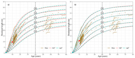
Figure 4.
Site index curves for the stands of patula pine with equation M2a and M2b at a base-age of 40 years. (a) altitude (2900 m), Tmin (5 °C), PTm (1200 mm), and slope (5%), (b) altitude (2200 m), Tmin (10 °C), PTm (900 mm), and slope (60%).
4. Discussion
Our results were consistent with Sharma et al. [67], who reported an improvement in fit with the addition of climatic variables (growing season mean temperature and growing season total precipitation) in the McDill-Amateis growth function [68] for jack pine (Pinus banksiana Lamb.) and black spruce (Picea mariana [Mill.] B.S.P.). Similarly, Bravo-Oviedo et al. [69] showed a fitting improvement and better model accuracy by including climatic variables (total autumn and winter precipitation and mean annual temperature) for maritime pine (Pinus pinaster Ait.) in four geographic regions of Spain. Oboite and Comeau [70] obtained better black spruce models when climatic variables (mean annual temperature and mean annual precipitation) were added to the equation developed by Huang and Titus [71] in four provinces of western Canada.
The R2adj values in the fitted models are consistent with those reported by Sánchez-González et al. [72], Quiñonez-Barraza et al. [73], Nava-Nava et al. [27], and Hipler et al. [74], who used the same fitting method. The AIC value decreased marginally with the addition of topographic and climatic variables for equation M2b (Table 4), suggesting that the fitted model is adequate for representing dominant tree height [75]. The correction of heteroscedasticity in the residuals allowed us to obtain adequate distributions, grouped at the zero-reference line (Figure 3).
By incorporating topographic and climatic variables in dominant height models, several learning opportunities appear; e.g., Mensah et al. [12] concluded this type of model represents an opportunity to learn about the behavior of forests in a changing environment. Another study, Leites et al. [76] mentioned that these models allow for a description of the response of the relationships among site variables, and at the same time, improved the prediction of forest site productivity [16] by distinguishing the abiotic feature differences between sites [77].
Other studies have reported that the Hossfeld IV GADA model is suitable for describing biological processes underlying tree growth [60,78], while Santiago-García et al. [79] pointed out that growth equations can be adapted to model different scenarios of climate change, enabling, for example, the modeling of forest growth with environmental variables.
The effect that topographic and climatic variables showed on the forest site productivity models fitted for patula pine suggests the consideration of our model (M2b) to improve site classification in the study area. This is because of the great contribution they had toward the model in explaining the response variable (p ≤ 0.05). That is, if the altitude increases and the Tmin decreases, there will be a reduction () in this variable, while if the PTm increases and the slope decreases, there will have a positive impact () (Table 4). The classification is relevant when it is related to stand yield, since a ±1 m difference in stand dominant height corresponds to approximately ±28 m3 ha−1 of commercial timber. Being aware of this knowledge would allow foresters to modify, if necessary, the prescription of silvicultural practices and production estimates related to sustainable forest management. This agrees with Özçelik et al. [56], who consider site index to play a major role in projecting future merchantable timber yield performance [7,9,25].
Site-specific topographic and climatic variables play an important role in the dominant height growth of patula pine stands, but not all the variables have the same effect on forest site productivity. Minimum annual mean temperature (Tmin) showed a positive effect on dominant height (r = 0.26, p ≤ 0.05) (Table 5), suggesting a better growth rate when Tmin values increased (Figure 4). This implies that patula pine grows better in warmer rather than colder conditions [80]. Warmer temperatures promote enzymatic activity and improve the efficiency of photosynthesis, which allows the accumulation of carbohydrates for distribution in the woody tissue [81].
The positive correlation of temperature with dominant height has been reported by several authors for different forest species. Messaoud and Chen [82] found this relationship in trembling aspen (Populus tremuloides Michx) and black spruce, as did Güner et al. [83] in black pine (Pinus nigra Arn. ssp. pallasiana (Lamb.) Holmboe). Bravo-Oviedo et al. [84] found a better productive performance of maritime pine in warmer sites. Additionally, in another analysis, Collalti et al. [85] stated that forest productivity increases as mean air temperatures increase.
The growth response of different forest species to temperature, as well as to other site-specific conditions, may vary. However, the studies cited above are consistent with an analysis conducted by Jandl et al. [86], who argued that only some forest species types will be strongly affected by climate change, or will demand immediate adaptations in their forest management plans.
Mean annual precipitation (PTm) showed a nonsignificant correlation with dominant height (Table 5), which indicates that for the study area, PTm is not a limiting factor for the growth rate of the dominant height of patula pine. This does not agree with Özel et al. [87], who found a positive correlation between productivity and precipitation in maritime pine. They highlighted that the species had better growth in areas with higher precipitation, which is consistent with the reports by Sanquetta et al. [88] and Elli et al. [15] for six hardwood species in Brazil. However, there are some studies that have reported no clear effects of precipitation over time; for example, Latta et al. [89].
Altitude showed a negative effect on forest site productivity (r = −0.31, p ≤ 0.05), suggesting a reduction in growth rate as altitude increased (Table 5 and Figure 4). This reduction will be a function of the parameter of the equation (M2b) that multiplies the ratio between the Tmin and altitude (Table 4). This finding suggests that patula pine does not develop adequately at high altitudes. In Mexico, patula pine is most often found at altitudes between 2100 and 2800 m [90]. A study conducted by Eimil-Fraga et al. [91] in Galicia, Spain, reported that maritime pine showed high growth rates at lower altitudes, related to relatively high temperatures. Several studies report these results. Álvarez-Álvarez et al. [92] found this relationship in maritime pine, and Yener and Altun [93] in oriental spruce (Picea orientalis L.), while Gülsoy and Çinar [94] reported a positive correlation for black pine in Turkey.
No significant relationship between dominant height and slope was detected (Table 5). However, 89% of the sampling plots are located on slopes <60%, indicating that the species grows best on moderate slope sites (Figure 4). Özel et al. [87] found similar behaviors for maritime pine; they indicated that the species grows best on sites with a slope of 20%–40%.
The results reported in our study indicate that climatic variables are essential factors for modeling the dominant height growth of patula pine, similar to results reported by other authors on different forest species [67,95]. Site variables were significant in explaining the variability in the dominant height growth pattern (Table 4, and Figure 2 and Figure 4), and they contribute to knowledge of the species’ ecology. The importance of the equation proposed in this study (M2b) lies in having an equation that can explain the dominant height growth dynamics with high credibility (Figure 4). In addition, our study provides a solid basis for improving decision-making in sustainable forest management by incorporating climate and topography attributes [63].
5. Conclusions
The inclusion of topographic (altitude and slope) and climate variables (mean annual precipitation and mean annual minimum temperature) in the fitted dominant height growth models of patula pine appears to modify the stand’s growth rate. Generally, forest site productivity was negatively affected at higher altitudes and lower temperatures, while lower altitudes and higher temperatures benefited dominant height growth. Our model may be used to accurately estimate the site index of patula pine stands, one of the most important elements for the correct planning of silvicultural treatments in managed forests for timber production and the optimization of the available resources of the site, in accord with its productive potential.
Author Contributions
Conceptualization: A.N.-N. and W.S.-G.; methodology: A.N.-N., G.Á.-P., W.S.-G., H.M.d.l.S.-P., J.R.V.-L. and G.Q.-B., formal analysis: A.N.-N., W.S.-G. and G.Q.-B.; investigation: A.N.-N. and W.S.-G.; resources: G.Á.-P. and W.S.-G.; writing—original draft preparation: A.N.-N., G.Á.-P. and W.S.-G.; writing—review and editing: A.N.-N., G.Á.-P., W.S.-G., H.M.d.l.S.-P., G.Q.-B. and J.R.V.-L. All authors have read and agreed to the published version of the manuscript.
Funding
This research was funded by The Mexican Council of Science and Technology (CONACYT) as a Doctoral fellowship of the first author, and by the community of Ixtlán de Juárez, Oaxaca, México who provided financial support to carry out this research.
Institutional Review Board Statement
Not applicable.
Informed Consent Statement
Not applicable.
Data Availability Statement
Data is available upon request to the corresponding authors.
Acknowledgments
We would like to acknowledge the National Council of Science and Technology (CONACYT) and the community of Ixtlán de Juárez, Oaxaca, México, for the facilities granted to carry out this research.
Conflicts of Interest
The authors declare no conflict of interest.
References
- Clutter, J.L.; Fortson, J.C.; Pienaar, L.V.; Brister, G.H.; Bailey, R.L. Timber Management: A Quantitative Approach; John Wiley & Sons Inc.: New York, NY, USA, 1983; p. 333. [Google Scholar]
- Allen, M.G.; Burkhart, H.E. A comparison of alternative data sources for modeling site index in loblolly pine plantations. Can. J. For. Res. 2015, 45, 1026–1033. [Google Scholar] [CrossRef]
- Sharma, M.; Parton, J. Climatic effects on site productivity of red pine plantations. For. Sci. 2018, 64, 544–554. [Google Scholar] [CrossRef]
- Kiviste, A.; Álvarez-González, A.; Rojo-Alboreca, A.; Ruiz-González, A.D. Funciones de Crecimiento de Aplicación en el Ámbito Forestal; INIA: Madrid, España, 2002; p. 190. [Google Scholar]
- Weiskittel, A.R.; Hann, D.W.; Kershaw, J.A.; Vanclay, J.K. Forest Growth and Yield Modeling; John Wiley & Sons: Chichester, UK, 2011; p. 430. [Google Scholar]
- Socha, J.; Tymińska-Czabańska, L.; Grabska, E.; Orzeł, S. Site index models for main forest-forming tree species in Poland. Forests 2020, 11, 301. [Google Scholar] [CrossRef]
- Kuehne, C.; McLean, P.; Maleki, K.; Antón-Fernández, C.; Astrup, R. A stand-level growth and yield model for thinned and unthinned even-aged Scots pine forests in Norway. Silva Fenn. 2022, 56, 10627. [Google Scholar] [CrossRef]
- Maleki, K.; Astrup, R.; Kuehne, C.; McLean, J.P.; Antón-Fernández, C. Stand-level growth models for long-term projections of the main species groups in Norway. Scand. J. For. Res. 2022, 37, 130–143. [Google Scholar] [CrossRef]
- Allen, M.G., II; Antón-Fernández, C.; Astrup, R. A stand-level growth and yield model for thinned and unthinned managed Norway spruce forests in Norway. Scand. J. For. Res. 2020, 35, 238–251. [Google Scholar] [CrossRef]
- Fiandino, S.; Plevich, J.; Tarico, J.; Utello, M.; Demaestri, M.; Gyenge, J. Modeling forest site productivity using climate data and topographic imagery in Pinus elliottii plantations of central Argentina. Ann. For. Sci. 2020, 77, 95. [Google Scholar] [CrossRef]
- Antón-Fernández, C.; Mola-Yudego, B.; Dalsgaard, L.; Astrup, R. Climate-sensitive site index models for Norway. Can. J. For. Res. 2016, 46, 794–803. [Google Scholar] [CrossRef]
- Mensah, S.; Pienaar, O.L.; Kunneke, A.; du Toit, B.; Seydack, A.; Uhl, E.; Pretzsch, H.; Seifert, T. Height—Diameter allometry in South Africa’s indigenous high forests: Assessing generic models performance and function forms. For. Ecol. Manag. 2018, 410, 1–11. [Google Scholar] [CrossRef]
- Tymińska-Czabańska, L.; Socha, J.; Hawryło, P.; Bałazy, R.; Ciesielski, M.; Grabska-Szwagrzyk, E.; Netzel, P. Weather-sensitive height growth modelling of Norway spruce using repeated airborne laser scanning data. Agric. For. Meteorol. 2021, 308–309, 108568. [Google Scholar] [CrossRef]
- Chen, H.Y.H.; Krestov, P.V.; Klinka, K. Trembling aspen site index in relation to environmental measures of site quality at two spatial scales. Can. J. For. Res. 2002, 32, 112–119. [Google Scholar] [CrossRef]
- Elli, E.F.; Caron, B.O.; Behling, A.; Eloy, E.; Queiróz De Souza, V.; Schwerz, F.; Stolzle, J.R. Climatic factors defining the height growth curve of forest species. iforest-Biogeosciences For. 2017, 10, 547–553. [Google Scholar] [CrossRef]
- Rachid-Casnati, C.; Mason, E.G.; Woollons, R.C. Using soil-based and physiographic variables to improve stand growth equations in Uruguayan forest plantations. iforest-Biogeosciences For. 2019, 12, 237–245. [Google Scholar] [CrossRef]
- Song, Y.; Sass-Klaassen, U.; Sterck, F.; Goudzwaard, L.; Akhmetzyanov, L.; Poorter, L. Growth of 19 conifer species is highly sensitive to winter warming, spring frost and summer drought. Ann. Bot. 2021, 128, 545–557. [Google Scholar] [CrossRef] [PubMed]
- Sharma, M. Climate effects on jack pine and black spruce productivity in natural origin mixed stands and site index conversion equations. Trees For. People 2021, 5, 100089. [Google Scholar] [CrossRef]
- Medlyn, B.E.; Duursma, R.A.; Zeppel, M.J.B. Forest productivity under climate change: A checklist for evaluating model studies. WIREs Clim. Chang. 2011, 2, 332–355. [Google Scholar] [CrossRef]
- Reyer, C. Forest productivity under environmental change—A review of stand-scale modeling studies. Curr. For. Rep. 2015, 1, 53–68. [Google Scholar] [CrossRef]
- Pau, M.; Gauthier, S.; Chavardes, R.D.; Girardin, M.P.; Marchand, W.; Bergeron, Y. Site index as a predictor of the effect of climate warming on boreal tree growth. Glob. Chang. Biol. 2022, 28, 1903–1918. [Google Scholar] [CrossRef]
- Achim, A.; Moreau, G.; Coops, N.C.; Axelson, J.N.; Barrette, J.; Bédard, S.; Byrne, K.E.; Caspersen, J.; Dick, A.R.; D’Orangeville, L.; et al. The changing culture of silviculture. For. Int. J. For. Res. 2022, 95, 143–152. [Google Scholar] [CrossRef]
- Bailey, R.L.; Clutter, J.L. Base-age invariant polymorphic site curves. For. Sci. 1974, 20, 155–159. [Google Scholar] [CrossRef]
- Cieszewski, C.J.; Bailey, R.L. Generalized algebraic difference approach: Theory based derivation of dynamic site equations with polymorphism and variable asymptotes. For. Sci. 2000, 46, 116–126. [Google Scholar] [CrossRef]
- Santiago-García, W.; Pérez-López, E.; Quiñonez-Barraza, G.; Rodríguez-Ortiz, G.; Santiago-García, E.; Ruiz-Aquino, F.; Tamarit-Urias, J. A dynamic system of growth and yield equations for Pinus patula. Forests 2017, 8, 465. [Google Scholar] [CrossRef]
- Castillo-López, A.; Santiago-García, W.; Vargas-Larreta, B.; Quiñonez-Barraza, G.; Solis-Moreno, R.; Corral Rivas, J.J. Dynamic site index models for four pine species in Oaxaca. Rev. Mex. Cienc. For. 2018, 9, 4–27. [Google Scholar] [CrossRef]
- Nava-Nava, A.; Santiago-García, W.; Rodríguez-Ortiz, G.; De los Santos-Posadas, H.M.; Ruiz-Aquino, F.; Santiago-García, E.; Suárez-Mota, M.E. Dynamic equations of growth in dominant height and site index for Pinus patula Schiede ex Schltdl. & Cham. Rev. Fitotec. Mex. 2020, 43, 470. [Google Scholar] [CrossRef]
- Santiago-García, W.; Jacinto-Salinas, A.H.; Rodríguez-Ortiz, G.; Nava-Nava, A.; Santiago-García, E.; Ángeles-Pérez, G.; Enríquez-del Valle, J.R. Generalized height-diameter models for five pine species at Southern Mexico. For. Sci. Technol. 2020, 16, 49–55. [Google Scholar] [CrossRef]
- Pérez-López, E.; Santiago-García, W.; Quiñonez-Barraza, G.; Rodríguez-Ortiz, G.; Santiago-García, E.; Ruiz-Aquino, F. Estimation of diameter distributions for Pinus patula with the Weibull function. Madera Bosques 2019, 25, e2531626. [Google Scholar] [CrossRef]
- Instituto Nacional de Estadística Geografía e Informática [INEGI]. Mapa de Edafología. Escala 1:250, 000. Mexico. 2000. Available online: https://www.inegi.org.mx/temas/edafologia/ (accessed on 10 June 2021).
- Servicios Técnicos Forestales de Ixtlán de Juárez [STF]. Programa de Manejo Forestal para el Aprovechamiento y Conservación de los Recursos Forestales Maderables de Ixtlán de Juárez. Ciclo de Corta 2015–2024; Servicios Técnicos Forestales de Ixtlán de Juárez: Oaxaca, Mexico, 2015; p. 423. [Google Scholar]
- Bates, J.M.; Granger, C.W.J. The Combination of forecasts. J. Oper. Res. Soc. 1969, 20, 451–468. [Google Scholar] [CrossRef]
- Timmermann, A. Chapter 4 Forecast combinations. In Handbook of Economic Forecasting; Elliott, G., Granger, C.W.J., Timmermann, A., Eds.; Elsevier: Amsterdam, The Netherlands, 2006; Volume 1, pp. 135–196. [Google Scholar]
- Petropoulos, F.; Apiletti, D.; Assimakopoulos, V.; Babai, M.Z.; Barrow, D.K.; Ben Taieb, S.; Bergmeir, C.; Bessa, R.J.; Bijak, J.; Boylan, J.E.; et al. Forecasting: Theory and practice. Int. J. Forecast. 2022, 38, 705–871. [Google Scholar] [CrossRef]
- Tait, D.E.; Cieszewski, C.J.; Bella, I.E. The stand dynamics of lodgepole pine. Can. J. For. Res. 1988, 18, 1255–1260. [Google Scholar] [CrossRef]
- SAS Institute. SAS/ETS® 9.3 User’s Guide; SAS Institute: Cary, NC, USA, 2011. [Google Scholar]
- Baltagi, B.H.; Heun Song, S.; Cheol Jung, B.; Koh, W. Testing for serial correlation, spatial autocorrelation and random effects using panel data. J. Econom. 2007, 140, 5–51. [Google Scholar] [CrossRef]
- Hsiao, C. Panel data analysis—Advantages and challenges. Test 2007, 16, 1–22. [Google Scholar] [CrossRef]
- Hsiao, C. Analysis of Panel Data, 3rd ed.; Cambridge University Press: Cambridge, UK, 2014; p. 539. [Google Scholar]
- Sarafidis, V.; Wansbeek, T. Cross-sectional dependence in panel data analysis. Econ. Rev. 2011, 31, 483–531. [Google Scholar] [CrossRef]
- Assman, E. The Principles of Forest Yield Study; Pergamon Press: Oxford, UK, 1970; p. 506. [Google Scholar]
- Alder, D. Estimación del Volumen Forestal y Predicción del Rendimiento, con Referencia Especial a los Trópicos; Organización de las Naciones Unidas para la Agricultura y la Alimentación: Roma, Italia, 1980; p. 118. [Google Scholar]
- Burkhart, H.E.; Tomé, M. Modeling Forest Trees and Stands; Springer: Berlin/Heidelberg, Germany, 2012; p. 458. [Google Scholar]
- Environmental Systems Research Institute [ESRI]. ArcGIS Desktop 10.2; Environmental Systems Research Institute: Redlands, CA, USA, 2014. [Google Scholar]
- Instituto Nacional de Estadística y Geografía [INEGI]. Continuo de Elevaciones Mexicano 3.0 (CEM 3.0). Mexico. 2017. Available online: https://www.inegi.org.mx/app/geo2/elevacionesmex/ (accessed on 10 November 2021).
- Thornton, M.M.; Shrestha, R.; Wei, Y.; Thornton, P.E.; Kao, S.; Wilson, B.E. Daymet: Annual Climate Summaries on a 1-km Grid for North America, Version 4; ORNL DAAC: Oak Ridge, TN, USA, 2020. [Google Scholar] [CrossRef]
- McNunn, G.; Heaton, E.; Archontoulis, S.; Licht, M.; VanLoocke, A. Using a crop modeling framework for precision cost-benefit analysis of variable seeding and nitrogen application rates. Front. Sustain. Food Syst. 2019, 3, 108. [Google Scholar] [CrossRef]
- Dorman, S.J.; Schürch, R.; Huseth, A.S.; Taylor, S.V. Landscape and climatic effects driving spatiotemporal abundance of Lygus lineolaris (Hemiptera: Miridae) in cotton agroecosystems. Agric. Ecosyst. Environ. 2020, 295, 106910. [Google Scholar] [CrossRef]
- Goulding, C.J. Validation of growth models used in forest management. N. Z. J. For. 1979, 24, 108–124. [Google Scholar]
- Vanclay, J.K.; Skovsgaard, J.P. Evaluating forest growth models. Ecol. Model. 1997, 98, 1–12. [Google Scholar] [CrossRef]
- Soares, P.; Tomé, M.; Skovsgaard, J.P.; Vanclay, J.K. Evaluating a growth model for forest management using continuous forest inventory data. For. Ecol. Manag. 1995, 71, 251–265. [Google Scholar] [CrossRef]
- R Core Team. R: A language and Environment for Statistical Computing; R Core Team: Vienna, Austria, 2021. [Google Scholar]
- Krumland, B.; Eng, H. Site Index Systems for Major Young-Growth Forest and Woodland Species in Northern California; California Department of Forestry & Fire Protection: Sacramento, CA, USA, 2005. [Google Scholar]
- Tewari, V.P.; Álvarez-González, J.G.; von Gadow, K. Dynamic base-age invariant site index models for Tectona grandis in peninsular India. South. For. A J. For. Sci. 2014, 76, 21–27. [Google Scholar] [CrossRef]
- Rojo-Alboreca, A.; Cabanillas-Saldaña, A.M.; Barrio-Anta, M.; Notivol-Paíno, E.; Gorgoso-Varela, J.J. Site index curves for natural Aleppo pine forests in the central Ebro valley (Spain). Madera Bosques 2017, 23, 143. [Google Scholar] [CrossRef]
- Özçelik, R.; Cao, Q.V.; Gómez-García, E.; Crecente-Campo, F.; Eler, Ü. Modeling dominant height growth of Cedar (Cedrus libani A. Rich) stands in Turkey. For. Sci. 2019, 65, 725–733. [Google Scholar] [CrossRef]
- Lopez-Senespleda, E.; Bravo-Oviedo, A.; Alonso Ponce, R.; Montero Gonzalez, G. Modeling dominant height growth including site attributes in the GADA approach for Quercus faginea Lam. in Spain. For. Syst. 2014, 23, 494–499. [Google Scholar] [CrossRef]
- Martín-Benito, D.; Gea-Izquierdo, G.; del Río, M.; Cañellas, I. Long-term trends in dominant-height growth of black pine using dynamic models. For. Ecol. Manag. 2008, 256, 1230–1238. [Google Scholar] [CrossRef]
- Durbin, J.; Watson, G.S. Testing for serial correlation in least squares regression. III. Biometrika 1971, 58, 1–19. [Google Scholar] [CrossRef]
- Molina-Valero, J.A.; Diéguez-Aranda, U.; Álvarez-González, J.G.; Castedo-Dorado, F.; Pérez-Cruzado, C. Assessing site form as an indicator of site quality in even-aged Pinus radiata D. Don stands in north-western Spain. Ann. For. Sci. 2019, 76, 113. [Google Scholar] [CrossRef]
- Kübler, D.; Hildebrandt, P.; Günter, S.; Stimm, B.; Weber, M.; Muñoz, J.; Cabrera, O.; Zeilinger, J.; Silva, B.; Mosandl, R. Effects of silvicultural treatments and topography on individual tree growth in a tropical mountain forest in Ecuador. For. Ecol. Manag. 2020, 457, 117726. [Google Scholar] [CrossRef]
- Tamarit-Urias, J.C.; Quiñonez-Barraza, G.; García-Cuevas, X.; Hernández-Ramos, J.; Monárrez-González, J.C. Dynamic equation to estimate the growth in diameter of Pinus montezumae Lamb. in Puebla, Mexico. Madera Bosques 2021, 27, e2732180. [Google Scholar] [CrossRef]
- Zhou, Y.; Lei, Z.; Zhou, F.; Han, Y.; Yu, D.; Zhang, Y. Impact of climate factors on height growth of Pinus sylvestris var. mongolica. PLoS ONE 2019, 14, e0213509. [Google Scholar] [CrossRef]
- Barrios-Trilleras, A.; López-Aguirre, A.M.; Báez-Aparicio, C.A. Modelamiento de la productividad de Gmelina arborea Roxb. con base en variables biofísicas y de rodal. Colomb. For. 2021, 24, 71–87. [Google Scholar] [CrossRef]
- Sharma, M.; Parton, J. Modelling the effects of climate on site productivity of white pine plantations. Can. J. For. Res. 2019, 49, 1289–1297. [Google Scholar] [CrossRef]
- Parresol, B.R.; Vissage, J.S. White Pine Site Index for the Southern Forest Survey; US Department of Agriculture, Forest Service, Southern Research Station: Asheville, NC, USA, 1998; Volume 10. [Google Scholar]
- Sharma, M.; Subedi, N.; Ter-Mikaelian, M.; Parton, J. Modeling climatic effects on stand height/site index of plantation-grown jack pine and black spruce trees. For. Sci. 2015, 61, 25–34. [Google Scholar] [CrossRef]
- McDill, M.E.; Amateis, R.L. Measuring forest site quality using the parameters of a dimensionally dompatible height growth function. For. Sci. 1992, 38, 409–429. [Google Scholar] [CrossRef]
- Bravo-Oviedo, A.; Tomé, M.; Bravo, F.; Montero, G.; del Río, M. Dominant height growth equations including site attributes in the generalized algebraic difference approach. Can. J. For. Res. 2008, 38, 2348–2358. [Google Scholar] [CrossRef]
- Oboite, F.O.; Comeau, P.G. Competition and climate influence growth of black spruce in western boreal forests. For. Ecol. Manag. 2019, 443, 84–94. [Google Scholar] [CrossRef]
- Huang, S.; Titus, S.J. An individual tree height increment model for mixed white spruce–aspen stands in Alberta, Canada. For. Ecol. Manag. 1999, 123, 41–53. [Google Scholar] [CrossRef]
- Sánchez-González, M.; Cañellas, I.; Montero, G. Base-age invariant cork growth model for Spanish cork oak (Quercus suber L.) forests. Eur. J. For. Res. 2008, 127, 173–182. [Google Scholar] [CrossRef]
- Quiñonez-Barraza, G.; De los Santos-Posadas, H.M.; Cruz-Cobos, F.; Velázquez-Martínez, A.; Ángeles-Pérez, G.; Ramírez-Valverde, G. Site index with complex polymorphism of forest stands in Durango, Mexico. Agrociencia 2015, 49, 439–454. [Google Scholar]
- Hipler, S.-M.; Spiecker, H.; Wu, S. Dynamic top height growth models for eight native tree species in a cool-temperate region in Northeast China. Forests 2021, 12, 965. [Google Scholar] [CrossRef]
- Burnham, K.P.; Anderson, D.R. Practical use of the information-theoretic approach. In Model Selection and Inference: A Practical Information-Theoretic Approach; Burnham, K.P., Anderson, D.R., Eds.; Springer: New York, NY, USA, 1998; pp. 75–117. [Google Scholar]
- Leites, L.P.; Robinson, A.P.; Rehfeldt, G.E.; Marshall, J.D.; Crookston, N.L. Height-growth response to climatic changes differs among populations of Douglas-fir: A novel analysis of historic data. Ecol. Appl. 2012, 22, 154–165. [Google Scholar] [CrossRef]
- Chiu, C.M.; Chien, C.T.; Nigh, G.D.; Chung, C.H. Climate and height growth of taiwania (Taiwania cryptomerioides) and Taiwan incense-cedar (Calocedrus formosana) in Taiwan. Forestry 2016, 89, 364–372. [Google Scholar] [CrossRef]
- Hernández-Cuevas, M.; Santiago-García, W.; De los Santos-Posadas, H.M.; Martínez-Antúnez, P.; Ruiz-Aquino, F. Models of dominant height growth and site indexes for Pinus ayacahuite Ehren. Agrociencia 2018, 52, 437–453. [Google Scholar]
- Santiago-García, W.; Ángeles-Pérez, G.; Quiñonez-Barraza, G.; De los Santos-Posadas, H.M.; Rodríguez-Ortiz, G. Advances and perspectives in modeling applied to forest planning in Mexico. Madera Bosques 2020, 26, e2622004. [Google Scholar] [CrossRef]
- van Zonneveld, M.; Jarvis, A.; Dvorak, W.; Lema, G.; Leibing, C. Climate change impact predictions on Pinus patula and Pinus tecunumanii populations in Mexico and Central America. For. Ecol. Manag. 2009, 257, 1566–1576. [Google Scholar] [CrossRef]
- Miyamoto, Y.; Griesbauer, H.P.; Scott Green, D. Growth responses of three coexisting conifer species to climate across wide geographic and climate ranges in Yukon and British Columbia. For. Ecol. Manag. 2010, 259, 514–523. [Google Scholar] [CrossRef]
- Messaoud, Y.; Chen, H.Y. The influence of recent climate change on tree height growth differs with species and spatial environment. PLoS ONE 2011, 6, e14691. [Google Scholar] [CrossRef] [PubMed]
- Güner, Ş.T.; Çömez, A.; Özkan, K.; Karataş, R.; Çelik, N. Türkiye’deki karaçam ağaçlandırmalarının verimlilik modellemesi. İstanbul Üniversitesi Orman Fakültesi Derg. 2016, 66, 166. [Google Scholar] [CrossRef]
- Bravo-Oviedo, A.; Roig, S.; Bravo, F.; Montero, G.; Del-Río, M. Environmental variability and its relationship to site index in Mediterranean maritine pine. For. Syst. 2011, 20, 50–64. [Google Scholar] [CrossRef]
- Collalti, A.; Ibrom, A.; Stockmarr, A.; Cescatti, A.; Alkama, R.; Fernandez-Martinez, M.; Matteucci, G.; Sitch, S.; Friedlingstein, P.; Ciais, P.; et al. Forest production efficiency increases with growth temperature. Nat. Commun. 2020, 11, 5322. [Google Scholar] [CrossRef] [PubMed]
- Jandl, R.; Spathelf, P.; Bolte, A.; Prescott, C.E. Forest adaptation to climate change—is non-management an option? Ann. For. Sci. 2019, 76, 48. [Google Scholar] [CrossRef]
- Özel, C.; Güner, Ş.T.; Türkkan, M.; Akgül, S.; Şentürk, Ö. Modelling the site index of Pinus pinaster plantations in Turkey using ecological variables. J. For. Res. 2021, 32, 589–598. [Google Scholar] [CrossRef]
- Sanquetta, C.R.; Behling, A.; Dalla Corte, A.P.; Pellico Netto, S.; Rodrigues, A.L.; Simon, A.A. A model based on environmental factors for diameter distribution in black wattle in Brazil. PLoS ONE 2014, 9, e100093. [Google Scholar] [CrossRef]
- Latta, G.; Temesgen, H.; Adams, D.; Barrett, T. Analysis of potential impacts of climate change on forests of the United States Pacific Northwest. For. Ecol. Manag. 2010, 259, 720–729. [Google Scholar] [CrossRef]
- Perry, J.P. The Pines of Mexico and Central America; Timber Press: Portland, OR, USA, 1991; p. 231. [Google Scholar]
- Eimil-Fraga, C.; Rodríguez-Soalleiro, R.; Sánchez-Rodríguez, F.; Pérez-Cruzado, C.; Álvarez-Rodríguez, E. Significance of bedrock as a site factor determining nutritional status and growth of maritime pine. For. Ecol. Manag. 2014, 331, 19–24. [Google Scholar] [CrossRef]
- Álvarez-Álvarez, P.; Khouri, E.A.; Cámara-Obregón, A.; Castedo-Dorado, F.; Barrio-Anta, M. Effects of foliar nutrients and environmental factors on site productivity in Pinus pinaster Ait. stands in Asturias (NW Spain). Ann. For. Sci. 2011, 68, 497–509. [Google Scholar] [CrossRef]
- Yener, I.; Altun, L. Predicting site index for oriental spruce (Picea orientalis L. (Link)) using ecological factors in the eastern black sea, Turkey. Fresenius Environ. Bull. 2018, 27, 3107–3116. [Google Scholar]
- Gülsoy, S.; Çinar, T. The Relationships between environmental factors and site index of anatolian black pine (Pinus nigra Arn. Subsp. pallasiana (Lamb.) Holmboe) Stands in Demirci (Manisa) District, Turkey. Appl. Ecol. Environ. Res. 2019, 17, 1235–1246. [Google Scholar] [CrossRef]
- Zang, H.; Lei, X.; Zeng, W. Height–diameter equations for larch plantations in northern and northeastern China: A comparison of the mixed-effects, quantile regression and generalized additive models. Forestry 2016, 89, 434–445. [Google Scholar] [CrossRef]
Publisher’s Note: MDPI stays neutral with regard to jurisdictional claims in published maps and institutional affiliations. |
© 2022 by the authors. Licensee MDPI, Basel, Switzerland. This article is an open access article distributed under the terms and conditions of the Creative Commons Attribution (CC BY) license (https://creativecommons.org/licenses/by/4.0/).