Abstract
So far, large-scale projects aiming to map forest attributes using aerial LiDAR data have been developed using ground sample plots acquired synchronously with LiDAR. No large projects have been developed using aerial LiDAR acquired independent of ground sample plot datasets. The goal of this study was to develop and validate large-scale parametric merchantable wood volume estimation models using existing historical ground sample plots. The models can be applied to large LiDAR datasets to map merchantable wood volume as a 10 × 10 m raster. The study demonstrated that a relative density index (RDI) based on a self-thinning equation and dominant height were suitable variables that can be calculated both for ground sample plots and LiDAR datasets. The resulting volume raster showed sound accuracy rates when compared to validation zones: R², 82.25%; RMSE, 13.7 m3/ha; and bias, −4.09 m3/ha. The results show that ground sample plot datasets acquired synchronously with LiDAR can be used to calculate the RDI and dominant height. These variables can consequently be used to map forest attributes over a large area with a high level of accuracy, thus not requiring the implementation of new costly sample plots.
1. Introduction
Airborne LiDAR (light detection and ranging) can be used to generate derivative products such as digital terrain models (DTMs) and canopy height models (CHMs). These derivative products are effectively used to support forest activities such as road building and harvesting [1,2,3,4]. The efficiency of using airborne LiDAR data to generate forest attributes has also been largely demonstrated [5,6,7,8]. The most common methods applied to predict forest attributes are based on either parametric or non-parametric models [9]. Parametric models can be parameterized using a finite number of parameters. These models also make several a priori assumptions about the relationships between response and predictor variables. Errors are normally distributed, independent, and have a constant variance.
On the other hand, non-parametric approaches make no restrictive assumptions and can include categorical dependent or independent variables. These non-parametric approaches, such as k-nearest neighbors or random forest, have been largely tested for estimating forest attributes based on LiDAR data [10,11].
Ideally, the prediction of forest attributes such as merchantable wood volume requires accurately located and representative ground sample plots. Several studies have demonstrated that ground sampling plans must fulfil several requirements such as representing the full variability range of the variables’ values, covering sufficient area, being accurately georeferenced, and minimizing the time delay between LiDAR acquisition and plot measurements [12,13,14,15,16]. These requirements for modeling approaches limit the operational use of LiDAR data for mapping forest attributes since the user generally has no control of LiDAR acquisition dates versus field work calendars. Moreover, forest attribute prediction approaches require expertise to ensure the representativeness, positioning accuracy, and synchronicity of ground sample plots. These issues reduce the high potential benefits of estimating forest attributes using LiDAR data.
In Québec (Canada), several thousand 400 m2 ground sample plots have been measured since the 1960s and entirely cover the province’s managed forests. Most of this huge dataset has been acquired for volume and other forest attribute calculations. Sample plots are measured synchronously with the province’s ecoforest mapping process, which takes approximately a ten-year cycle to complete. In this context, this ground sample plot dataset can be potentially used to develop a general forest attribute parametric model for which independent variables can be subsequently linked to recent LiDAR metrics and ecoforest map attributes. Such models are advantageous, as they ensure that the ecological tendencies are taken into account and, once developed for an area, these models overcome ground sample plot measurement requirements such as positioning accuracy and synchronicity with LiDAR [17]. However, because of the frequent time gap between ground sample plot measurements and LiDAR acquisitions, no large-scale parametric models have yet been developed using LiDAR acquired independent of ground sample plot datasets to ultimately produce merchantable wood volume maps using LiDAR data.
Thus, the goals of this study are (i) to develop and validate forest attribute models that can be calculated simultaneously on a ground plot database and on LiDAR datasets using plots acquired synchronously with LiDAR and, consequently, (ii) to develop and validate large-scale parametric merchantable wood volume estimation models using existing historical ground sample plots that can finally be applied over large LiDAR datasets to map merchantable wood volume.
2. Materials and Methods
2.1. Study Area
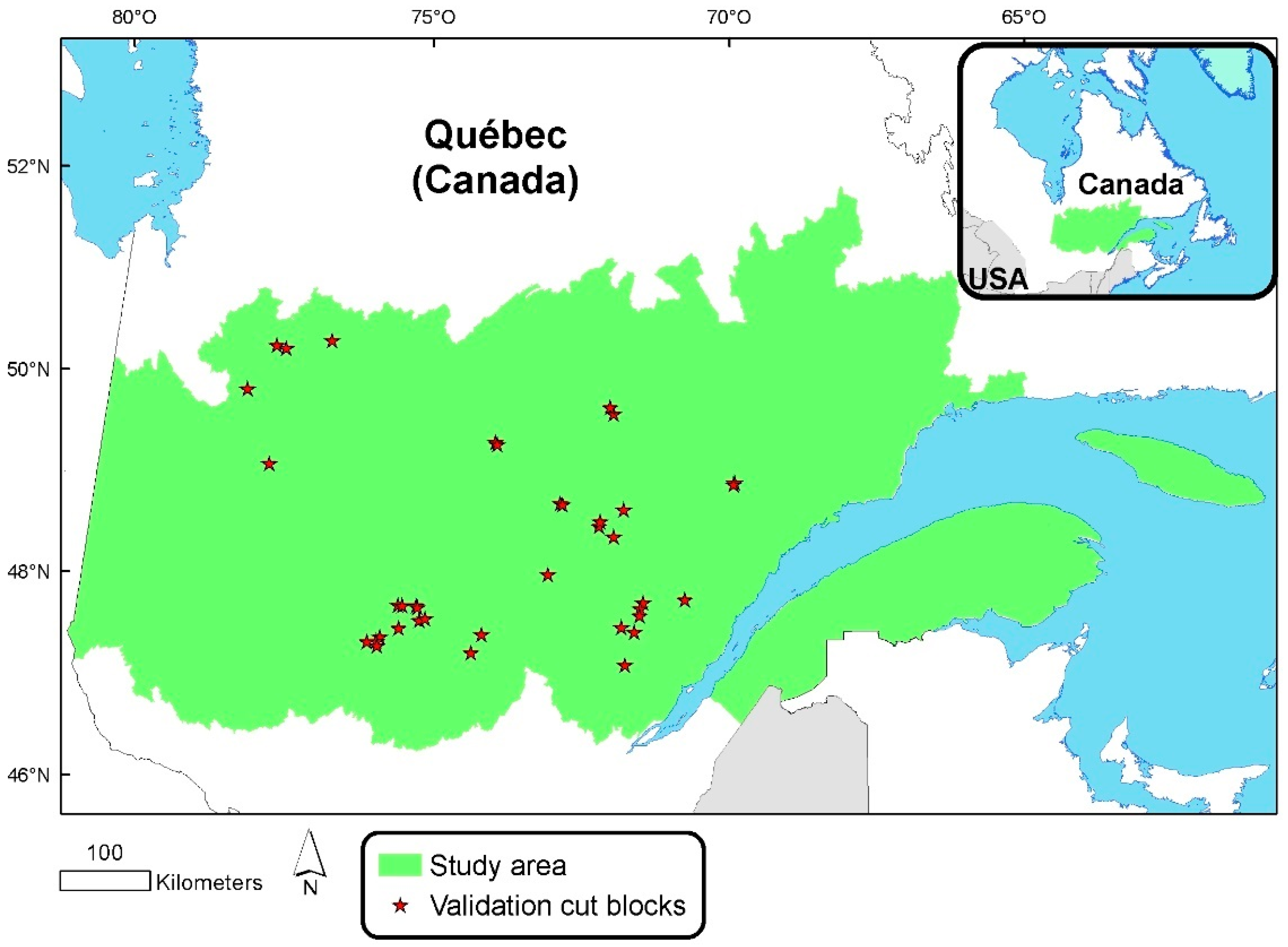
The study area is located in the spruce–feathermoss, fir–white birch, and fir–yellow birch bioclimatic domains of Québec [18] in eastern Canada (Figure 1). These are included in the eastern boreal forests and eastern temperate mixed forests of Canada [19].
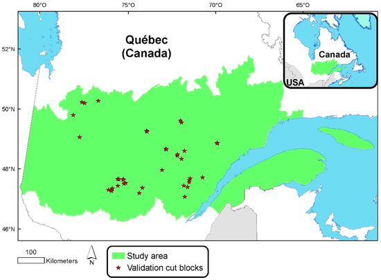
Figure 1.
Location of the study area in Québec (Canada) and validation cut blocks (red stars).
The study area covers about 440,000 km² between the 47th and 52nd parallels, an area exceeding twice the size of Finland. Forests vary importantly in the study area, following latitudinal and longitudinal ecological gradients. The forest species in the dryer and colder north-west portion of the study area consist mainly of black spruce (Picea mariana (Mill.) B.S.P.) and jack pine (Pinus banksiana Lamb.), two species that are generally located on landscapes affected by recurrent forest fires. The understories in this area are usually dominated by ericaceous shrubs, mosses, and lichens in varying proportions. Balsam fir (Abies balsamea (L.) Mill.) proportions are higher in the east, where precipitations are higher and fire events less frequent. Thus, in the north-east portion of the study area, zonal sites are dominated by black spruce and balsam fir with a feather moss understory. Further south, the slightly warmer climate favors balsam fir-, white birch (Betula papyrifera Marsh.)-, and white spruce (Picea glauca (Moench) Voss)-dominated stands on zonal sites, accompanied by black spruce and trembling aspen (Populus tremuloides Michx.) with herbaceous, shrub, or feathermoss understories. Yellow birch appears in the southernmost portions of the study area. Lastly, altitudinal and coastal areas can be dominated by white spruce due to increased humidity.
The landscape consists of rolling terrain as well as more rugged hills reaching elevations of 1000 mASL (maximum altitude is 1268 m). The mean annual temperature varies from −1.1 °C to −10.8 °C, resulting in a short growing season (between 78 and 155 days), and the mean annual precipitation varies from 201 to 1200 mm per year. The surficial deposits of most of the study area are dominated by glacial till.
2.2. Data
2.2.1. Airborne LiDAR Data
By 2021, the Québec government had covered most of the province’s managed forest with airborne LiDAR data. Thus, several airborne LiDAR datasets were available, which were acquired between 2011 and 2020. The sensors used were all linear-mode with a wavelength of 1064 nm but had different characteristics, as described in Table 1.

Table 1.
Characteristics of the airborne LiDAR acquisition parameters used in this study.
2.2.2. Ground Sample Plots
The study area was covered by 41,472 ground sample plots measured between 2003 and 2018 by the Ministère des Forêts, de la Faune et des Parcs of Québec. Ground sample plots were randomly located in forest stands higher than or equal to 7 m. The plots were circular, with a radius of 11.28 m, covering 400 m² and required a ≤3.57 m positional accuracy, ensuring co-registration with the LiDAR data [20,21]. The diameter at breast height (DBH) (diameter at 1.3 m including bark thickness) was measured for all trees in a ground sample plot having a DBH higher than 9 cm. For these trees, the species was also recorded.
In each ground sample plot, study trees were randomly selected [21]. For these trees, height was measured with an accuracy of 10 cm. Each ground sample plot was associated with a corresponding landscape unit based on their geographic coordinates. Landscape units [22] represent local ecological homogeneity and dynamics and are largely used in operational forestry. The study area covers 77 landscape units. Some units have been merged to ensure that at least 50 ground sample plots were in each unit.
2.2.3. Ground Plots Synchronous with LiDAR
Among the 41,472 ground sample plots, 2285 plots were measured within about 5 growing seasons of the LiDAR acquisitions, with an average difference of 0.5 growing seasons. These 2285 ground plots synchronous with LiDAR (synchronous ground plots) cover a large ecological gradient and were used for the relative density index calibration model.
2.2.4. Cut Blocks
As an independent validation dataset, 38 cut blocks (shown in Figure 1) were available to obtain accurate measures of harvested wood volumes. The mean area of these cut blocks was 361 ha, varying from 51 to 2858 ha. The site selection followed these considerations: harvested less than five growing seasons after the LiDAR acquisition date, have accurate measures of harvested and non-harvested wood volume, and represent a large range of forest types. The harvesting contours of each site were delimited based on aerial photographs acquired after the harvesting operations. The harvestable merchantable volume was calculated using mass–volume equations [23]. Moreover, the volume of unused woody debris left on the sites was estimated from postcut inventories [24].
2.2.5. Ecoforest and Ecological Land Classification
Forest inventories and mapping in Québec began in 1970. Québec’s manageable forests are fully inventoried and mapped using aerial photo-interpretation within an approximately 10 year cycle. The fifth ecoforest inventory began in 2015. An ecological inventory was also conducted between 1985 and 2000 and was used to produce an ecological land classification. For this study, data from the fourth and fifth inventories were used as well as certain levels of the recently updated ecological land classification [18,25,26,27].
2.3. Ground Sample Plots Compilation
2.3.1. Dominant Height Ground Sample Plot Compilations
The dominant height of the ground sample plots (DH_plot) followed plot measurement guidelines [28,29]. First, a threshold was established as 66% of the mean height of the study trees defined as dominant and co-dominant. Second, for all trees higher than this threshold, the mean weighted height using the basal area was calculated. In the case where more than 16 trees were higher than the threshold, the weighted height was performed only on the 16 highest trees.
2.3.2. Dependent Variables
First, volume was calculated at tree level. The merchantable volume was calculated using existing general equations [30] that were adapted to extract non-usable parts of the tree. Specifically, the volume of trees between diameters of 9 cm without bark and 9 cm with bark was not considered, even though it was initially considered in the databases. This adapted tree level equation required two variables: the diameter at breast height (DBH), which was measured for each tree in the ground sample plots, and the height, which was estimated using a height-DBH equation [31]. The merchantable volume was defined as the volume of each portion of the trunk and branches between the stump (15 cm from the ground) and the minimal diameter fit for sawing (9 cm at the smallest diameter without bark). The total volume (without bark) considered all portions of the tree up to the tips of the branches, including the apex.
Second, these tree volumes were summed for all the trees in each ground sample plot. Three different volumes were calculated: the merchantable volume for all species (vALL_plot), the total volume for all species above a threshold of 5 m (v5_plot), and the commercial coniferous merchantable volume (vFSPL_plot). A v5_plot was chosen as the dependent variable because the height threshold values were highly related to the merchantable volume, which can be applied to both the ground and LiDAR datasets. Based on our ground sample plots dataset, over this threshold of 5 m, in some cases, trees produced merchantable volume. Under this threshold of 5 m, in no case was merchantable volume was observed. The FSPL includes the following commercial tree species: balsam fir, black spruce, white spruce, jack pine, and larch (Larix laricina (Du Roi) K. Koch). These species were chosen based on their high commercial value on the North American market. Finally, the number of stems higher than 5 m (stem5_plot) was also calculated. Table 2 describes the range of values of the ground sample plot volume compilation.
Table 2.
Calculated dependent variables and their significations and ranges of values.
2.4. Independent Variables Preparation
For all independent variables, 10 × 10 m resolution rasters were produced. A 20 × 20 m spatial resolution was evaluated so it would be as similar as possible to the size of the ground sample plots (400 m²) following best practices [9], but preliminary results demonstrated that 10 × 10 m cells improved the final results, especially when taking into account heterogeneous forests and forests adjacent to harvested areas. All produced rasters were created from a common master raster to avoid misalignment between them.
The method aimed to calculate metrics, based on LiDAR data, that maximize the correlation, both for coniferous/deciduous or low/high stands, with the dominant and mean height measured for the ground plots. Several LiDAR metrics were tested using ground plots synchronous with LiDAR.
In order to produce the first 10 × 10 m resolution raster, the dominant height (DH_LiDAR), several methodological steps were tested to maximize the correlation with the dominant height from the ground plots. First, a canopy height model (CHM) was created by subtracting the digital terrain model (DTM) from the canopy surface model (CSM) using a 1 m spatial resolution. The Lasgrid and Las2dem algorithms from LAStools were applied. The resulting CHM_1m was then adjusted by using the models by Fradette et al. [32] to reduce the height bias caused by differences in pulse density over the study area. A maximal focal statistic was first applied to CHM_1m to identify the highest value in a circle neighborhood analysis. Several radiuses (3, 4, 5, 6, and 7 m) and tree height values (from 7 to 20 m) were tested. The resulting raster was CHM_1m_FOC. The results of these iterations are presented in Section 3.1. The DH_LiDAR was finally calculated as the mean of all CHM_1m_FOC pixels contained in the 10 × 10 m pixel.
In the case of the second 10 × 10 m resolution raster, the mean height above 5 m (MH5_LiDAR), several methodological steps were tested to maximize the correlation with the calculated relative density index (RDI), which is described later in this section. First, a Lasthin (LASTools) was performed directly on the raw lidar data (.las files). The chosen resolution (step variable) was 0.3 m pixels since this fit with the LiDAR mean pulse density over the study area. Then, other algorithm variables were tested. Several circle radiuses (0.2, 0.4, and 0.6 m) were tested according to the tree height because this influences the crown diameter and the distance between trees [33] for three cover types (coniferous, mixed, and deciduous) for the ecoforest map. Next, Lasheight (LAStools, Rapidlasso GmbH, Gilching, Germany) and Las2dem (LAStools, Rapidlasso GmbH, Gilching, Germany) were applied to finally obtain a 1 m resolution raster. This raster was also adjusted by using the models by Fradette et al. [32] to reduce the height bias. Finally, the mean value of all pixels higher than 5 m was calculated for all 10 × 10 m pixels. The NoData pixels were ignored to calculate the mean. The results of this iteration are also presented in Section 3.1.
First, the correlation between DH_LiDAR and DH_plot was evaluated for all synchronous ground plots to ensure that there was no significant difference with the 1:1 line.
In order to find optimal independent variables applicable to both plots and LiDAR data, we performed preliminary tests using synchronous datasets with several different LiDAR acquisition parameters. These tests indicated that an RDI produces the most stable results among the LiDAR datasets, even though the acquisition parameters differed (pulse density, sensor type, scan angles, etc.).
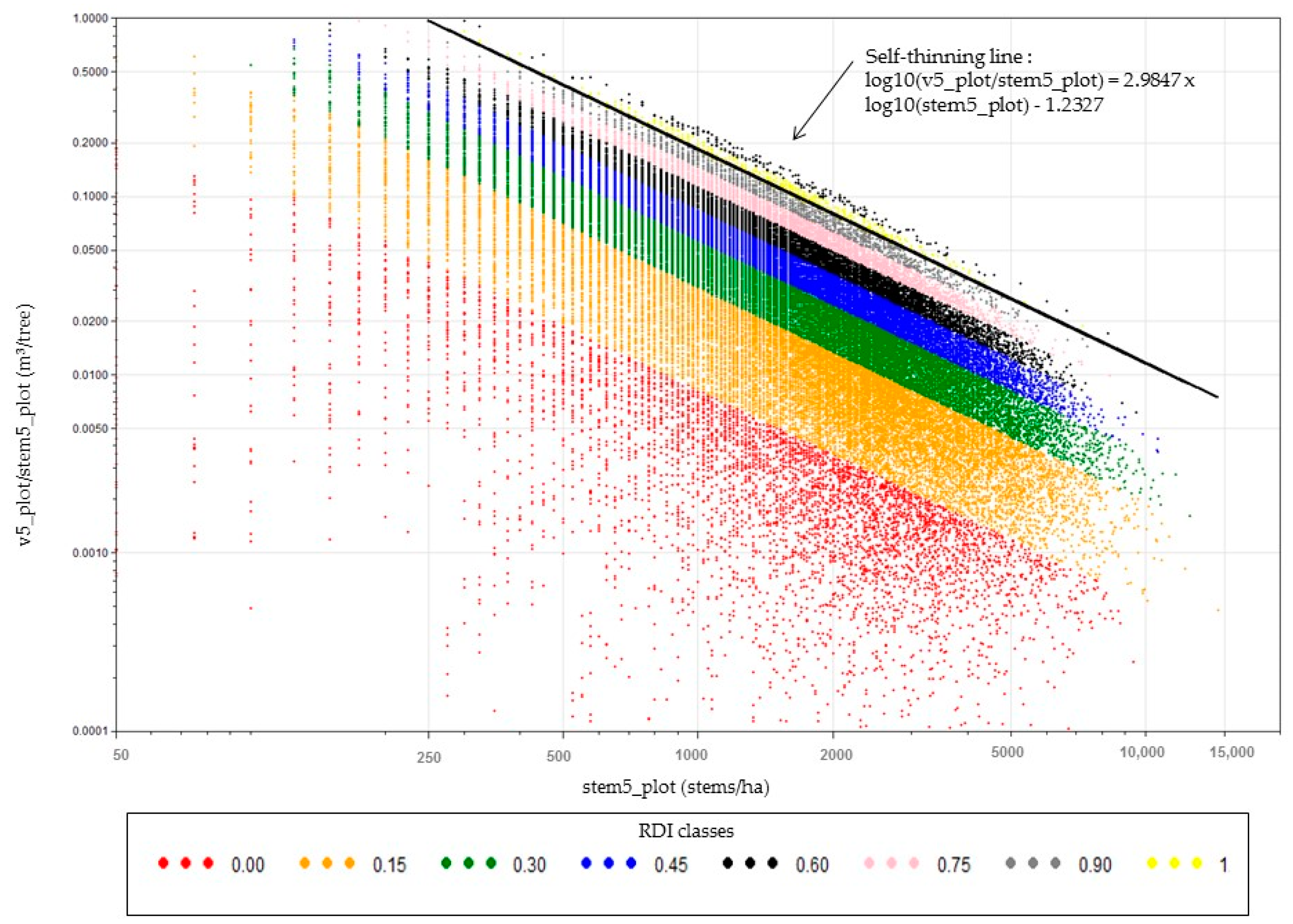
Calculating an RDI required several steps. First, a self-thinning line was calibrated for the whole study area with all the available (41,472) ground sample plots. Quantile regression model equations for the 99th quantile were used so that 1% of the ground sample plots were above the line and 99% were below the line. For the self-thinning regression, the dependent variable was the v5_plot divided by the number of stems above 5 m (m3/tree), and the independent variable was the stem5_plot. A logarithmic scale was used due to the density’s exponential effect on the volume.
Equation (1) shows the self-thinning line equation:
where m and b are self-thinning line parameters.
Log10(v5_plot/stem5_plot) = m × log10(stem5_plot) + b
Second, with the self-thinning line, an RDI value was calculated for each synchronous ground plot. The calculated RDI was obtained by dividing the observed stem5_plot by the stem5_plot resulting from the self-thinning equation.
An RDI model was made to predict RDI values for 10 × 10 m raster cells (predicted RDI). To create this model, the RDI calculated from synchronous ground plots were associated with DH_LiDAR, MH5_LiDAR, and DTM from overlaid 10 × 10 m raster cells. A height difference (DELTA_H) was added as an independent variable to the equation to consider the time delay between LiDAR acquisition and plot measurements. This variable was obtained from a height growth model adapted from Laflèche et al. [34]. Then, a log-linear model was used to obtain the log10 (RDI) in order to maintain the assumption of normality. Next, to correct the bias of the exponential value, a nonlinear regression was used to obtain the antilog model (RDI) [35]. With the final model, a predicted RDI raster was produced for the whole study area. A Bayesian information criteria (BIC) analysis was performed to avoid overfitting in the model. Finally, since we aimed to create a model generally predicting crown closure, species, age, and understory were not considered.
Finally, five 10 × 10 m rasters were made from the polygonal ecoforest map: dominant species, FSPL proportion (pFSPL_map), standard version of the map (PERC), landscape units, and bioclimatic subdomains, these last two variables both being part of the provincial ecological land classification [18]. Throughout the years, the improved resolution of the aerial photos used to produce the ecoforest map has resulted in two different mapping standards used for species photo-interpretation in the study area [25,26,27]. Thus, the accuracy of the pFSPL_ map varies in portions of the study area depending on the year each portion was mapped. This variation was considered by establishing either 0.1 or 0.25 classes for the different mapping standards within the binary raster named PERC.
2.5. Prediction Models
This crucial methodological step aimed to create models from the 41,472 ground sample plots dataset that can further be applied over the 10 × 10 m raster produced in the previous step. Thus, independent variables had to be calculated both using (i) the ground sample plots dataset and (ii) only the LiDAR and map variables. Two models were created to optimize the relation between (i) the dependent variable (vALL_plot or vFSPL_plot) and (ii) the independent variables from Section 2.3 (DH_plot) and Section 2.4 (calculated RDI, DTM, and ecoforest map variables). These two resulting models were: vALL (all species merchantable volume) and pFSPL (the proportion of FSPL merchantable volume). To obtain the FSPL merchantable volume (vFSPL), a multiplication of the two models was necessary (vALL × pFSPL).
A stepwise linear regression was performed. The linear effect model was selected among others in order to simplify the process and validate the tendencies. To develop such models, we first tested that the dependent variables were normally distributed. Secondly, we tried several combinations and interactions of variables based on both the Akaike information criteria (AIC) and logical aspects.
2.6. Volume Prediction Mapping
Values for vALL and vFSPL were calculated for each 10 × 10 m pixel throughout the study area using the prediction models developed in Section 2.5 and applied to the rasters of the independent variables in Section 2.4 (predicted RDI, DH_LiDAR, DTM, etc.). Three rasters were created, vALL, pFSPL, and vFSPL.
2.7. Volume Validation
Thirty-eight cut blocks were used to validate vFSPL. Since vFSPL was the result of the multiplication of the two models (vALL × pFSPL), these two models were also indirectly validated. The comparison was made by summing the values of the 10 × 10 m pixels whose centroid was included within a cut block contour. This sum was compared to the measured value in the cut block.
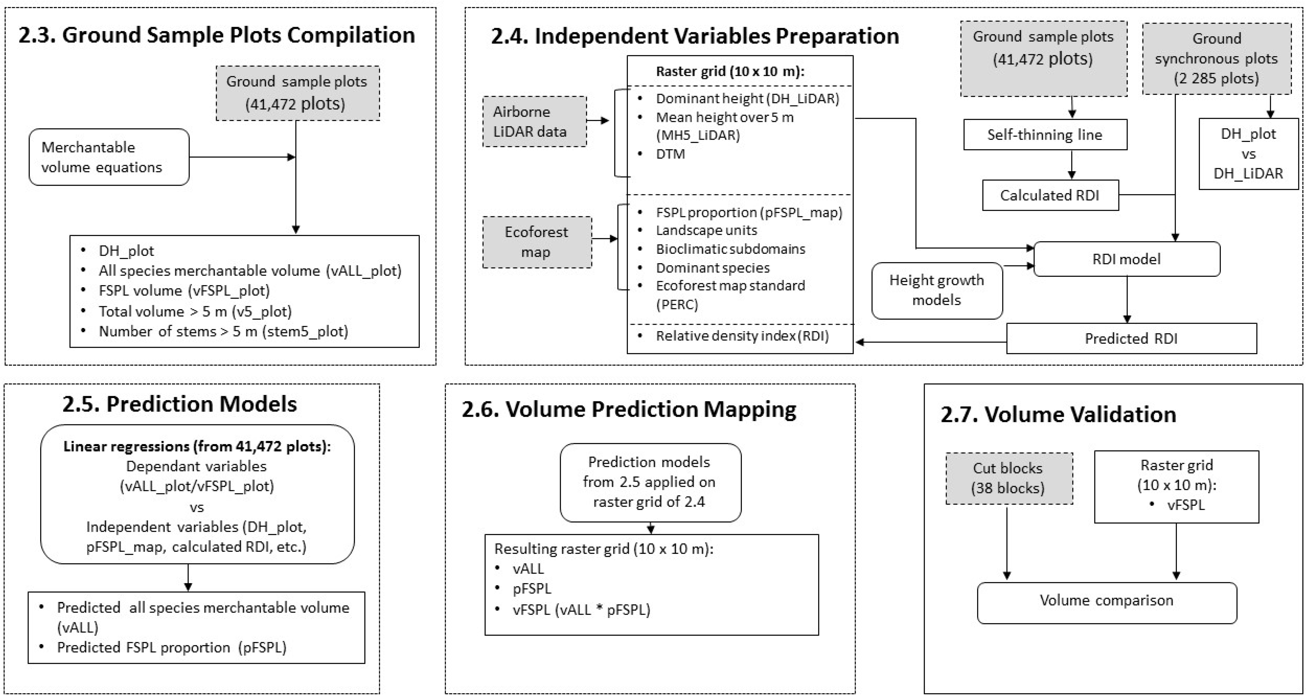
Figure 2 summarizes the developed method.
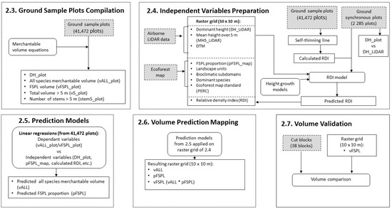
Figure 2.
Method summary.
3. Results
3.1. LiDAR Preparation Data
For DH_LiDAR, the optimal circle neighborhood radius was, respectively, 4, 5, and 6 m for trees higher or equal to 17 m, 11 to 16.99 m, and 0 to 10.99 m. For the MH5_LiDAR, 5 m indicated the optimal correlation. Thus, 5 m was subtracted from each of the CHM_1m pixels to obtain the mean height above 5 m (CHM_1m_5). The optimal results were obtained when different radiuses were applied for coniferous, mixed, or deciduous stands in order to artificially enlarge coniferous crowns. In coniferous stands, eight points were systematically added around each selected point in a radius of 0.4 m. In mixed stands, eight points were systematically added around each selected point in a radius of 0.2 m. No points were added for deciduous stands.
3.2. DH_plot vs. DH_LiDAR
No significant difference with the 1:1 line was found between DH_LiDAR and DH_plot. In this case, DH_plot was used to calibrate the vALL and pFSPL models, and DH_LiDAR was then applied to the 10 × 10 rasters.
3.3. RDI
3.3.1. RDI Self-Thinning
Figure 3 shows the self-thinning line for the study area. Each point represents a ground sample plot. The colors in the legend represent the proposed percentile classes of the RDI values and show the slope of the self-thinning line.

Figure 3.
Self-thinning line for the study area.
3.3.2. RDI Model
Equation (2) shows the result of the log-linear model. The R² of the model was 85.89%.
where adjust_t_RDI (Equation (3)) represents the adjustment for growing season differences between the LiDAR and ground sample plots:
where DELTA_H is the result (positive or negative height value (m)) of the growing model for which the growing season difference (year of ground plot—year of LiDAR) was applied.
logRDI = −1.7512 + ajust_t_RDI + (−0.04888 × MH5_LiDAR/100) + (1.3410 × log10 (MH5_LiDAR/100)) + (0.03567 × (DH_LiDAR/100)) + (0.000424 × DTM) + (−0.00037 × DTM × log10 (MH5_LiDAR/100))
ajust_t_RDI = DELTA_H × 0.1717 + (−0.00533 × DELTA_H × (DH_LiDAR/100))
It is well-demonstrated that log-linear models generate biased predictions after anti-log transformation [36,37]. To obtain the unbiased RDI prediction, a nonlinear regression was developed. Thus, the predictions of logRDI needed to be corrected using Equation (4):
3.4. Prediction Models
Equations (5) and (6), respectively, show the results of the all species merchantable volume and FSPL proportion linear regression:
where β0–β20 are the model parameters; DH corresponds to DH_plot because there is no significant difference with DH_LiDAR (Section 3.2); and RDI is the calculated RDI from the self-thinning line.
vALL = β0 + β1 × DTM + β2 × DH + β3 × DH × RDI + β4 × DH × pFSPL_map + β5 × RDI + β6 × RDI × DTM + β7 × RDI × RDI/DH + β8 × RDI/DH + β9 × (RDI/DH) ² + β10 × pFSPL_map
pFSPL = β11 + β12 × DH + β13 × PERC + β14 × pFSPL_map + β15 × pFSPL_map × DH + β16 × pFSPL_map × PERC + β17 × pFSPL_map ² + β18 × pFSPL_map ² × DH + β19 × pFSPL_map 3 + β20 × pFSPL_map 3 × PERC
The R² values of the vALL and pFSPL models were, respectively, 97.0% and 69.7%.
For the two prediction models, some parameters depend on the landscape unit (β0, β5, β8, β11, β12, and β14), bioclimatic subdomain (β0, β9, β11, β13, and β17) and dominant species (β0, β1, β5, β8, β9, β11, β12, and β13). Parameters have been determined for 94 landscape units, 5 bioclimatic subdomains, and 12 dominant species.
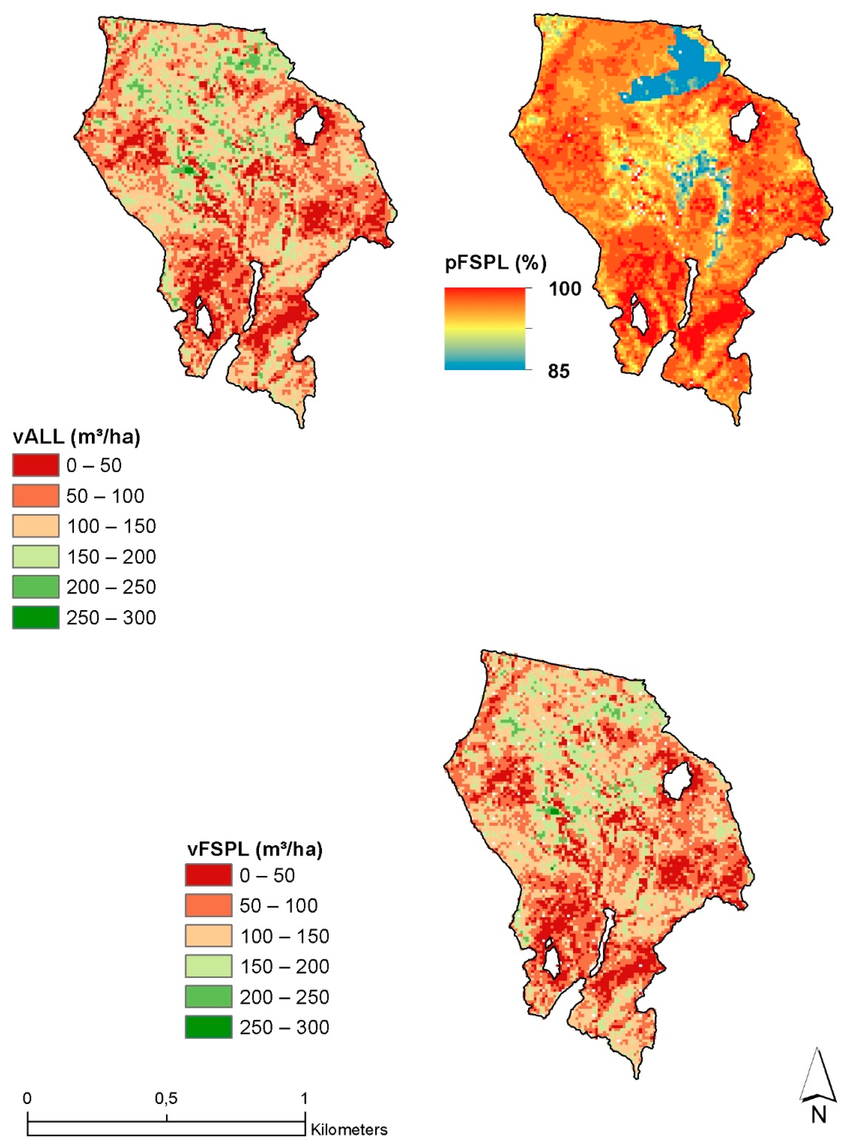
Figure 4 shows the result for a cut block.

Figure 4.
Example of volume for all species (vALL) and volume FSPL (vFSPL) raster maps produced for a specific area. vFSPL is the multiplication of pFSPL and vALL. Lower volume values are in red, and higher volume values are presented in green. For pFSPL, lower FSPL proportions are presented in blue, and higher proportions are presented in red.
3.5. Validation
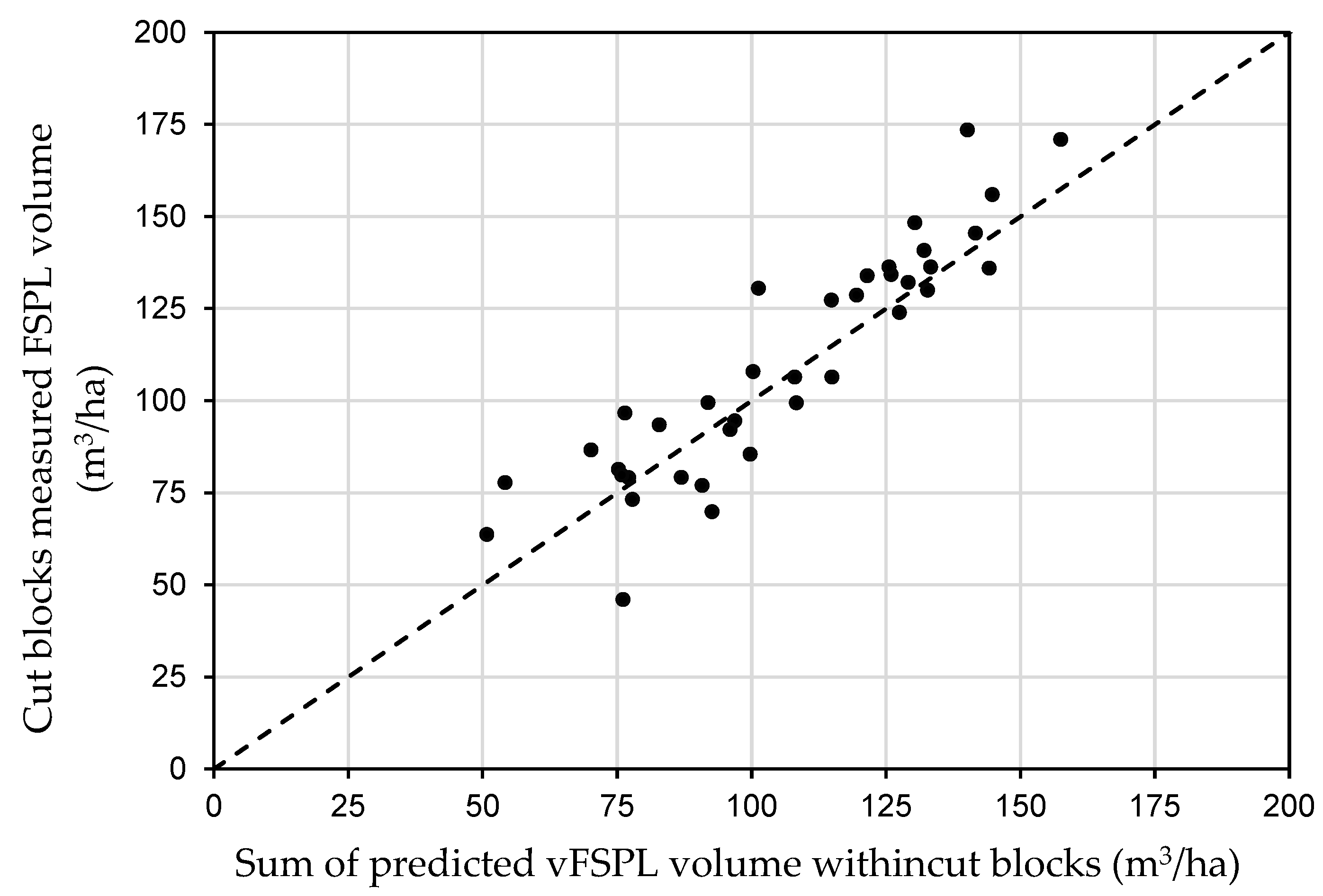
Figure 5 shows the comparison between vALL and vFSPL in the cut blocks. Most of the cut blocks are close to the 1:1 line. R², RSME, and the mean bias are, respectively, 82.25%, 13.7 m3/ha, and −4.09 m3/ha.
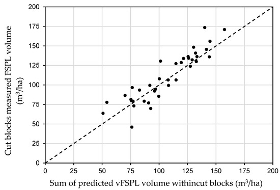
Figure 5.
Measured FSPL volume compared to predicted volume values from models (vFSPL) within cut blocks.
4. Discussion
A key novelty of this study lies in the identification of variables that can be calculated both for ground sample plots and LiDAR datasets. The RDI and dominant height proved to be the most suitable variables. The framework presented herein provides an approach to obtain accurate forest volume estimates using LiDAR data. Moreover, once the parametric prediction models are developed, no new ground sample plots are required to map volumes for a large spectrum of forest conditions.
We anticipate that this approach can support other organizations that want to map volumes with a high level of accuracy using LiDAR without needing new costly ground sample plot acquisition programs. Despite this innovation, this approach requires the consideration of several issues.
First, the approach required existing plot datasets. Ideally, these plots must cover multiple forest conditions. Moreover, a part of this dataset should be acquired in approximately the same growing season as the LiDAR data. These synchronous ground plots were needed to develop the RDI models. Second, the approach was developed using linear-mode LiDAR. However, the pulse density varied within the dataset, and this variability can bring variable bias in the height values over the LiDAR dataset. This issue was addressed by applying the models developed by Fradette et al. [32] that were also based on linear-mode LiDAR. Finally, the same area must be covered by ecoforest maps to provide information on the main forest species located in the resulting volume pixels.
There are also some limits to consider for expanding such an approach to other contexts. First, the fact that forest height underestimation increases as the pulse density decreases has been demonstrated [38,39]. However, it is recommended to either calculate a local correction model or to be sure that the LiDAR dataset pulse density is dense and relatively uniform over the area. Consequently, it is not recommended to use leaf-off LiDAR acquisitions. In such acquisitions, tree height underestimation could bring significant bias. Second, the accuracy of the pFSPL model was weaker (69.7%) compared to vALL (97%). This weaker result is mainly explained by the fact that we used the ecoforest map information to determine the proportions of each species. In fact, species proportions are interpreted over a larger polygon than the resulting spatial resolution and consequently can induce certain inaccuracies. This weakness could, however, be reduced by improving species accuracies in terms of spatial resolution and proportion estimates. Third, the window of applicability of such an approach depends on the range of forest conditions covered by the ground sample plots. In our case, the approach is applicable for commercial stands only since ground sample plots were located in stands higher or equal to 7 m. Finally, our study area mainly covered boreal forests where the main species are coniferous or shade-intolerant deciduous. The accuracy rates could be lower for shade-tolerant deciduous species since tree height–diameter allometry is weaker [40] than for coniferous species or for shade-intolerant deciduous species. These shade-tolerant deciduous species are located mainly south of the study area.
Despite the limits highlighted previously, this is a sound approach for calculating forest volumes for boreal forest commercials stands. To improve the practicality of this work for forest managers and practitioners, the approach based on parametric models could be developed and validated for other key forest attributes such as diameters, basal areas, biomass, etc.
5. Conclusions
Effectively predicting a large range of forest attributes with LiDAR data has been widely demonstrated. The commonly used approach is a non-parametric one requiring sample plots with accurate geographic coordinates measured synchronously with LiDAR acquisition [41]. This study has demonstrated that RDI and dominant height are two variables that can be used to link ground sample plot attributes to LiDAR metrics. These developments paved the way to use existing ground sample plot datasets to build a robust parametric dendrometric model. These models can be subsequently applied to LiDAR data and map forest attributes with a high level of accuracy. This approach can ultimately reduce or even avoid the requirement of new costly ground sample plots. While this approach has proven it effectiveness for boreal forest commercial stands, other forest conditions and attributes should be tested to define its range of applicability.
Author Contributions
Conceptualization, D.M.; methodology, D.M., M.R. and A.L.; data processing, D.M.; predictive models, M.R. and J.B.; formal analysis, M.R. and M.-S.F.; original draft preparation, A.L., M.R., D.M., M.-S.F. and J.B.; writing—review and editing, A.L. and M.R. All authors have read and agreed to the published version of the manuscript.
Funding
This research received no external funding.
Institutional Review Board Statement
Not applicable.
Informed Consent Statement
Not applicable.
Data Availability Statement
The volume maps produced by this study are openly available at (https://www.donneesquebec.ca/recherche/dataset/carte_dendrometrique_lidar), accessed on 20 March 2022, with a CC_BY 4.0 license.
Acknowledgments
This project was undertaken by the Direction des inventaires forestiers of the Ministère des Forêts, de la Faune et des Parcs du Gouvernement du Québec. The authors thank Mélanie Major for the revision and advise. The authors also thank Bureau de Mise en Marché des Bois, Ministère des Forêts, de la Faune et des Parcs, and forest industries for the cut block datasets.
Conflicts of Interest
The authors declare no conflict of interest.
References
- MFFP. Guide D’utilisation des Produits Dérivés du LiDAR. Available online: https://mffp.gouv.qc.ca/documents/forets/inventaire/guide-interpretation-lidar.pdf (accessed on 16 September 2021).
- Hyyppä, J.; Yu, X.; Hyyppä, H.; Vastaranta, M.; Holopainen, M.; Kukko, A.; Kaartinen, H.; Jaakkola, A.; Vaaja, M.; Koskinen, J.; et al. Advances in Forest Inventory Using Airborne Laser Scanning. Remote Sens. 2012, 4, 1190–1207. [Google Scholar] [CrossRef] [Green Version]
- Treitz, P.; Lim, K.; Woods, M.; Pitt, D.; Nesbitt, D.; Etheridge, D. Lidar Sampling Density for Forest Resource Inventories in Ontario, Canada. Remote Sens. 2012, 4, 830–848. [Google Scholar] [CrossRef] [Green Version]
- Wulder, M.A.; Bater, C.W.; Coops, N.C.; Hilker, T.; White, J.C. The role of Lidar in sustainable forest management. Forest Chron. 2008, 84, 807–826. [Google Scholar] [CrossRef] [Green Version]
- Bouvier, M.; Durrieu, S.; Fournier, R.A.; Renaud, J.-P. Generalizing predictive models of forest inventory attributes using an area-based approach with airborne Lidar data. Remote Sens. Environ. 2015, 156, 322–334. [Google Scholar] [CrossRef]
- Means, J.; Acker, S.; Fitt, B.; Renslow, M.; Emerson, L.; Hendrix, C. Predicting forest stand characteristics with airborne scanning LiDAR. PE&RS 2000, 66, 1367–1371. [Google Scholar]
- Næsset, E. Predicting forest stand characteristics with airborne scanning laser using a practical two-stage procedure and field data. Remote Sens. Environ. 2002, 80, 88–99. [Google Scholar] [CrossRef]
- Woods, M.; Pitt, D.; Penner, M.; Lim, K.; Nesbitt, D.; Etheridge, D.; Treitz, P. Operational implementation of a Lidar inventory in Boreal Ontario. For. Chron. 2011, 87, 512–528. [Google Scholar] [CrossRef]
- NRCAN. A Best Practices Guide for Generating Forest Inventory Attributes from Airborne Laser Scanning Data Using an Area-based Approach. Available online: https://cfs.nrcan.gc.ca/publications/download-pdf/34887 (accessed on 30 September 2021).
- Hudak, A.T.; Crookston, N.L.; Evans, J.S.; Hall, D.E.; Falkowski, M.J. Nearest neighbor imputation of species-level, plot-scale forest structure attributes from LiDAR data. Remote Sens. Environ. 2008, 112, 2232–2245. [Google Scholar] [CrossRef] [Green Version]
- McInerney, D.; Nieuwenhuis, M. A comparative analysis of kNN and decision tree methods for the Irish National Forest Inventory. Int. J. Remote Sens. 2009, 30, 4937–4955. [Google Scholar] [CrossRef]
- Adams, T.; Brack, C.; Farrier, T.; Pont, D.; Brownlie, R. So you want to use Lidar? A guide on how to use Lidar in forestry. N. Z. J. For. 2011, 55, 19–23. [Google Scholar]
- Frazer, G.W.; Magnussen, S.; Wulder, M.A.; Niemann, K.O. Simulated impact of sample plot size and co-registration error on the accuracy and uncertainty of Lidar-derived estimates of forest stand biomass. Remote Sens. Environ. 2011, 115, 636–649. [Google Scholar] [CrossRef]
- Montgomery, D.C.; Peck, E.A.; Vining, G.G. Introduction to Linear Regression Analysis, 5th ed.; John Wiley & Sons: New York, NY, USA, 2006; 672p. [Google Scholar]
- Magnussen, S.; Næsset, E.; Gobakken, T. Reliability of Lidar derived predictors of forest inventory attributes: A case study with Norway spruce. Remote Sens. Environ. 2010, 114, 700–712. [Google Scholar] [CrossRef]
- Gobakken, T.; Næsset, E. Assessing effects of laser point density, ground sampling intensity, and field sample plot size on biophysical stand properties derived from airborne laser scanner data. Can. J. For. Res. 2008, 38, 1095–1109. [Google Scholar] [CrossRef]
- Coops, N.C.; Tompalski, P.; Goodbody, T.R.H.; Queinnec, M.; Luther, J.E.; Bolton, D.K.; White, J.C.; Wulder, M.A.; Van Lier, O.R.; Hermosilla, T. Modelling lidar-derived estimates of forest attributes over space and time: A review of approaches and future trends. Remote Sens. Environ. 2021, 260, 112477. [Google Scholar] [CrossRef]
- MFFP. Classification Écologique du Territoire Québécois. Available online: https://mffp.gouv.qc.ca//documents/forets/inventaire/classification_ecologique_territoire_quebecois.pdf (accessed on 23 November 2021).
- Baldwin, K.; Allen, L.; Basquill, S.; Chapman, K.; Downing, D.; Flynn, N.; MacKenzie, W.; Major, M.; Meades, W.; Meidinger, D.; et al. Vegetation Zones of Canada: A Biogeoclimatic Perspective; Information Report, GLC-X-25; Canadian Forest Service: Sault Ste Marie, ON, Canada, 2021. [Google Scholar]
- MFFP. Normes D’inventaire Forestier: Placettes-Échantillons Permanentes. Available online: https://mffp.gouv.qc.ca/documents/forets/inventaire/norme-5e-inventaire-peppdf.pdf (accessed on 16 September 2021).
- MFFP. Normes D’inventaire Écoforestier: Placettes-Échantillons Temporaires. Available online: https://mffp.gouv.qc.ca/documents/forets/inventaire/Norme_PET_5e.pdf (accessed on 16 September 2021).
- Robitaille, A.; Saucier, J.-P. Paysages Régionaux du Québec Méridional; Les Publications du Québec: Québec, QC, Canada, 1998; 213p. [Google Scholar]
- MRNF. Méthodes de Mesurage des Bois. Instructions Techniques. Exercice 2011–2012. Available online: https://numerique.banq.qc.ca/patrimoine/details/52327/21117?docref=BXYItiZ193KhaBXrjEGF3w (accessed on 16 September 2021).
- MRN. Inventaire de la Matière Ligneuse Utilisable Mais non Récoltée dans les Aires de Coupe. Instructions. Available online: https://mffp.gouv.qc.ca/publications/forets/entreprises/matli.pdf (accessed on 16 September 2021).
- MFFP. Norme de Stratification Écoforestière, Quatrième Inventaire Écoforestier du Québec Méridional. Available online: https://mffp.gouv.qc.ca/documents/forets/inventaire/norme-stratification.pdf (accessed on 30 September 2021).
- MFFP. 5e Inventaire Écoforestier du Québec Méridional, Bilan des Orientations Retenues et des Travaux de mise en Oeuvre. Available online: https://mffp.gouv.qc.ca/documents/forets/inventaire/bilan-orientations.pdf (accessed on 30 September 2021).
- MFFP. Cartographie du Cinquième Inventaire Écoforestier du Québec Méridional. Available online: https://mffp.gouv.qc.ca/documents/forets/inventaire/carto_5E_methodes_donnees.pdf (accessed on 30 September 2021).
- Rondoux, J. La Mesure des Arbres et des Peuplements Forestiers; Les Presses de l’Université de Liège: Liège, Belgium, 2021; 737p. [Google Scholar]
- IUFRO. The Standardization of Symbols in Forest Mensuration; Technical Bulletin 15; University of Maine, Agricultural Experimental Station: Orono, ME, USA, 1965; 32p. [Google Scholar]
- Fortin, M.; DeBlois, J.; Bernier, S.; Blais, G. Mise au point d’un tarif de cubage général pour les forêts québécoises: Une approche pour mieux évaluer l’incertitude associée aux prévisions. For. Chron. 2007, 83, 754–765. [Google Scholar] [CrossRef]
- Auger, I. Une Nouvelle Relation Hauteur-Diamètre Tenant Compte de L’influence de la Station et du Climat Pour 27 Essences Commerciales du Québec. Available online: https://mffp.gouv.qc.ca/documents/forets/connaissances/recherche/Note146.pdf (accessed on 30 September 2021).
- Fradette, M.-S.; Leboeuf, A.; Riopel, M.; Bégin, J. Method to Reduce the Bias on Digital Terrain Model and Canopy Height Model from LiDAR. Remote Sens. 2019, 11, 863. [Google Scholar] [CrossRef] [Green Version]
- Franceschi, S.; Antonello, A.; Floreancig, V.; Gianelle, D.; Comiti, F.; Tonon, G. Identifying tree tops from aerial laser scanning data with particle swarming optimization. Eur. J. Remote Sens. 2018, 51, 945–964. [Google Scholar] [CrossRef] [Green Version]
- Laflèche, V.; Bernier, S.; Saucier, J.-P.; Gagné, C. Indices de Qualité de Station des Principales Essences Commerciales en Fonction des Types Écologiques du Québec Méridional. Available online: https://mffp.gouv.qc.ca/documents/forets/inventaire/indices-qualite.pdf (accessed on 30 September 2021).
- Girard, C.; Ouarda, T.; Bobée, B. Étude du biais dans le modèle log-linéaire d’estimation régionale. Can. J. Civ. Eng. 2004, 31, 361–368. [Google Scholar] [CrossRef]
- Finney, D.J. On the distribution of a variate whose logarithm is normally distributed. J. Roy. Stat. Soc. Suppl. 1941, 7, 155–161. [Google Scholar] [CrossRef]
- Beauchamp, J.J.; Olson, J.S. Corrections for Bias in Regression Estimates After Logarithmic Transformation. Ecology 1973, 54, 1403–1407. Available online: https://can01.safelinks.protection.outlook.com/?url=https%3A%2F%2Fdoi.org%2F10.2307%2F1934208&data=05%7C01%7CAntoine.Leboeuf%40mffp.gouv.qc.ca%7C4e70f28818044606cb3908da23b6d1f4%7C8705e97737814f4790e1c84c8b884da1%7C0%7C0%7C637861565349383242%7CUnknown%7CTWFpbGZsb3d8eyJWIjoiMC4wLjAwMDAiLCJQIjoiV2luMzIiLCJBTiI6Ik1haWwiLCJXVCI6Mn0%3D%7C3000%7C%7C%7C&sdata=B%2BbAmOJski%2FWJP4u0R%2Fe%2F7LVkG2sxLMneRSWftB0J%2F4%3D&reserved=0 (accessed on 30 September 2021). [CrossRef]
- Yu, X.; Hyyppä, J.; Hyyppä, H.; Maltamo, M. Effects of flight altitude on tree height estimation using airborne laser scanning. Arch. Photogramm. Remote Sens. Spat. Inf. Sci. 2004, 36, 96–101. [Google Scholar]
- Næsset, E.; Okland, T. Estimating tree height and tree crown properties using airborne scanning laser in a boreal nature reserve. Remote Sens. Environ. 2002, 79, 105–115. [Google Scholar] [CrossRef]
- Hulshof, C.; Swenson, N.; Weiser, M. Tree height–diameter allometry across the United States. Ecol. Evol. 2015, 6, 1193–1204. [Google Scholar] [CrossRef] [PubMed]
- White, J.; Coops, N.; Wulder, M.; Vastaranta, M.; Hilker, T.; Tompalski, P. Remote Sensing Technologies for Enhancing Forest Inventories: A Review. Can. J. Remote Sens. 2016, 42, 619–641. [Google Scholar] [CrossRef] [Green Version]
Publisher’s Note: MDPI stays neutral with regard to jurisdictional claims in published maps and institutional affiliations. |
© 2022 by the authors. Licensee MDPI, Basel, Switzerland. This article is an open access article distributed under the terms and conditions of the Creative Commons Attribution (CC BY) license (https://creativecommons.org/licenses/by/4.0/).