Abstract
Although Land Surface Temperatures (LSTs) are on the rise globally, the distribution of LSTs varies depending on the land cover type. Urban Heat Island and Urban Cool Island effects act differently, especially in semi-arid regions. Therefore, we identify demi-decadal, seasonal, and zonal differences in LSTs in a semi-arid region in the city of Jaipur, where zones include rural and urban areas that encircle the Jhalana Reserve Forest (JRF). After deriving LSTs from remotely sensed thermal bands of Landsat satellites’ Multi-spectral datasets, we found that there is a significant difference in LST (p < 0.01) among the zones. In addition, LSTs were found to be significantly lower in JRF compared to Urban and Rural areas in all seasons and all study years, which indicates the urban cooling effect due to the presence of the forest. Nevertheless, summer LSTs have warmed with a mean difference of 4.8 °C between 2000 and 2020. Therefore, our study supports the promotion of Urban Forests, especially in semi-arid zones, for inculcating LST regulation ecosystem services to enrich and enhance the standard of living of the human population.
1. Introduction
Anthropogenic activities have resulted in extensive changes in land use patterns (industrialization, urbanization, deforestation, agriculture diversification, etc.), which further alter regional micro-climates [1]. One of the most conspicuous is the Land Surface Temperatures (LST) which are on the rise globally. LST is defined as “the temperature felt when the land surface is touched with the hands” [2]. Urbanization is one of the major factors contributing to the change in land use and land cover (LULC) patterns and which plays a role in the regulation of regional or local climates [3,4].
The Urban Heat Island (UHI) is “a phenomenon whereby temperatures within a city or large towns are often significantly higher than those of surrounding rural areas” [5,6,7].
UHI effects are observed in most of the urban areas of the world [8,9,10,11,12,13,14] and in Indian cities as well [15,16,17]. In contrast, urban areas or the city cores with extensive vegetated areas exhibit the Urban Cool Island (UCI) effect, wherein the daytime surface temperatures are lower than the surrounding anthropogenically modified areas [18,19]. The phenomenon has not been extensively studied, especially in arid and semi-arid areas [20,21,22].
Vegetation density has been shown to have a strong negative correlation with LSTs and vice versa [23,24,25,26,27], wherein vegetation reduces the intensity of the UHI effect by providing evapotranspiration and shade cooling, i.e., UCI [28,29]. Similarly, urban forests are responsible for significantly reducing the UHI effect, especially during warm periods [30,31,32].
Irrigation in the semi-arid area affects LSTs significantly [33,34]. For example, irrigated paddy fields in semi-arid regions of Jilin province of China, studied between 2005–2017, with data collected from regional land-use, remote sensing, and metrology analyzed LST changes, with radiative and non-radiative changes, found the largest temperature change during the dry summer months of July and August. Irrigated fields also displayed strong negative correlations with LSTs [34]. Further, amongst the most significant mitigants of UHI and related health risks were ecological services provided by urban forests [35,36]. Ecosystem services are defined as those benefits which are obtained by humans as a product of an ecosystem function [37]. Ecosystem services are also the end products of some ecosystem function which is valuable to human populations in a beneficial way, such as climate regulation or recreation [38]. It was shown that although green areas reduce LST when they are not cultivated, the LST values increase considerably.
Jaber and Abu-Allaban [39] studied MODIS-based daytime and night-time LSTs for Jordan with semi-arid to arid environments and found the highest LST values in June and lowest in December. They also found that human populations had a greater effect than natural factors (elevation). In another study in the semi-arid cities of Ahmedabad and Gandhinagar in India, based on 12 MODIS satellite images, LSTs were analyzed with Normalized Difference Vegetation Index (NDVI), Normalised Difference Builtup Index (NDBI), and Impervious surface fraction (ISF); and developed a model based on these indices to improve the correlation of the LSTs between the day and the night. UHI effect was observed during the night in both cities [40]. Guha and Govil [41] studied the spatiotemporal relationship between LST and NDVI for Raipur (21.2514° N, 81.6296° E), which is in a tropical wet (Savannah) type climatic region of central India. To measure the LST and NDVI, cloud-free Landsat data of the pre-monsoon season from 2002–2018 were analyzed, and strong negative relationships between LSTs and NDVI throughout the study area were found. However, negative values of NDVI showed a positive and inconsistent relationship of LST-NDVI [41]. Similarly, in another study in Jordan, based on a one-year (2017) MODIS data set, results indicated a weak relation between LST (diurnal and nocturnal) and NDVI for the four different seasons (winter, spring, summer, and fall) [42]. However, they did find significant variation between the seasons and land cover class or vegetation classification (cropland, grassland, urban areas, and barren land). Further, the surface UCI effect was observed during the daytime in the urban areas. These studies stress how anthropogenic activities affect LST distribution while natural vegetation helps regulate and even reduce LST.
The fact that vegetated areas, whether as cultivated fields or urban parks, reduce LST in human-dominated landscapes shows that LST can be regulated to suit human comfort zones. Hence, our objective was to quantify the effect of a relatively large urban forest, which is a protected area, on the urban micro-climate of the surrounding urban areas in a hot semi-arid climatic region. We undertook a quantitative analysis of the relationships between the three zones to examine the seasonal effects of LST. We hypothesized that the forest area, now encircled by the conurbation of the city of Jaipur and other rural villages, will accord ecosystem services to the residents by acting as a heat sink.
The ecosystem services associated with JRF are listed below (Table 1). These services are based on published literature related to JRF.

Table 1.
List and types of ecosystem services mentioned or obtained through recent studies.
2. Materials and Methods
2.1. Study Area
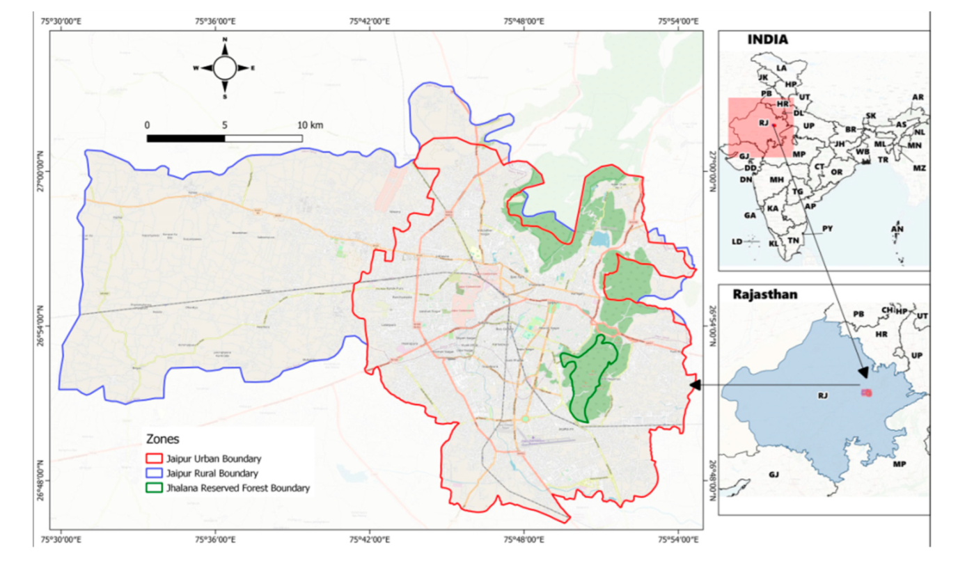
Our study compared LSTs of the Jhalana Reserve Forest (JRF; 26.8619° N, 75.8171° E; also named the Jhalana Leopard Reserve) and the conurbation of Jaipur, Rajasthan, India (Figure 1 and Figure 2). Jaipur is the capital city of the state of Rajasthan. JRF was once the private hunting grounds of the Maharaja of Jaipur and was declared a protected area in May 2017. It has a total area of 29 km2 and is now a green island encircled by the city of Jaipur [43,44,45]. Jaipur and all the satellite villages combined have an estimated population of 5 million residents. During the 1980s, the main valley was planted with Acacia tortilis and Acacia senegal. Altitudes vary between 280 m in the South to 530 m in the North-East. JRF has no buffer or core areas and only has a 2 m wall with a 3 m fence above it that separates the forested area from the urban neighborhoods and villages. JRF is characterized by a tropical dry deciduous forest. The climate of this region is described as Semi-Arid Hot Steppe Climate (Bsh) by the Köppen–Geiger climate classification [46].
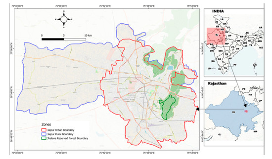
Figure 1.
Map of the study area showing the Urban (red), Rural (blue), and Jhalana Reserve Forest (green) zones of the conurbation of Jaipur.
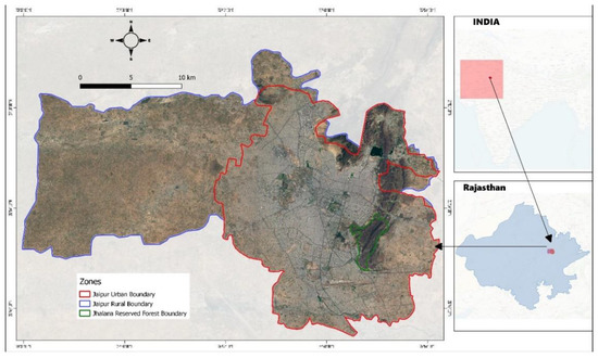
Figure 2.
Satellite map of the study area showing the Urban (red), Rural (blue), and Jhalana Reserve Forest (green) zones of the conurbation of Jaipur. The IMD (Indian Meteorological Department) records the meteorological variables continuously at weather stations, including at Jaipur (Sanganer) weather station (Table 2; [23]). Map courtesy of TGIS laboratory.
The IMD (Indian Meteorological Department) records the meteorological variables continuously at weather stations, including at Jaipur (Sanganer) weather station Table 2 [49].
Table 2.
The average maximum and minimum ambient temperatures (°C) and average precipitation for the conurbation of Jaipur.
2.2. Data Collection
Mean daytime LST data were utilized for this study for three different seasons, i.e., summer, monsoon, and winter, of every fifth year, i.e., encompassing a total of 15 seasons over 20 years (2000, 2005, 2010, 2015, and 2020). We considered summer to be from April to June, monsoon from July–September, and winter from October to March.
For LST measurement and analysis, various methods and approaches have been applied by different authors [50,51,52]. Satellite sensor data of Landsat–5 (Thematic Mapper), Landsat–7 (Enhanced Thematic Mapper Plus), and Landsat–8 (Operational Land Imager and Thermal Infrared Scanner) imagery are utilized for measurement of surface temperature and analyzing biophysical parameters [53]. ASTER (Advanced Spaceborne Thermal Emission and Reflection Radiometer) and MODIS (Moderate Resolution Imaging Spectroradiometer) satellite data were also used to measure LST in Saudi Arabia [54]. MODIS has the advantage that its night-time data is able to identify UHI effects in these areas. However, because MODIS has a very low resolution as compared to Landsat LST data, we chose Landsat thermal bands based LST computations for our analyses.
2.3. Data Processing
In this study, we used a mono-window algorithm to derive LSTs from Thermal bands of Landsat sensors. Thermal bands for Landsat 5 and 7, i.e., Band 6 (10.40–12.50 μm wavelength), were used for retrieving LSTs for the study years 2000, 2005, and 2010, whereas for Landsat 8, Band 10 (10.6–11.19 μm wavelength) was used for 2015 and 2020. As Landsat 7 had an SLC (Scan Line Corrector) failure since May 2003, the gaps in the images were also filled using average NDVI, i.e., mean cell raster value of different images of the respective seasons but of variable date using ‘Cell Statistics’ tool in QGIS. All these bands were resampled to 30m resolution for uniformity in analysis. Additionally, interpolation was performed to fill the ‘no data’ gaps (no data may have resulted from cloud cover) in a few of the LST rasters wherever required. Basically, all the suitable Landsat images available during the respective seasonal periods were taken, and their mean was derived by using raster cell statistics mentioned earlier.
Further mosaicing and subsetting were carried out as required for deriving LST rasters fitting in the study area. The quantile method was used for the visualization of LST maps.
2.4. Data Analysis and Analysis Categories
In addition, the analysis was conducted based on administrative zones in order to elucidate the zone variability of the LSTs. Zones were delineated based on digitization and procurement of vector data. The city boundary was used to delimit the urban areas, and the remaining Jaipur Tehsil (administrative division outside the city limits) was considered a rural zone. The JRF boundary was vectorized prior to analysis for a separate zone. Thus, we made a comprehensive assessment of LSTs for the Jaipur region based on demi-decadal, seasonal and zonal variations analysis. The demi-decadal analysis included analysis for the Summer, Monsoon, and Winter seasons in each of the 5 years, and the seasonal analysis included the data mentioned for each season. Lastly, Zonal analysis refers to spatial variations of LSTs based on the three zones (Table 3).
Table 3.
Land Surface Temperature analysis types and components.
2.5. Statistical Techniques
For statistical analysis, 100 random points (i.e., 300 random points for each LST map) were included in the study for each zone for all years and seasons. Random points spread across the zones were generated, pixel-based values of LSTs were extracted and tabulated, and statistical analysis was conducted. Density plots were prepared to understand the LST distribution according to all the three analysis types, i.e., seasonal, zonal, and year-wise. Moreover, category-wise p-values were computed using the Kruskal-Wallis ANOVA test to check for statistically significant differences between the category values since the data does not have fixed parameters and hence cannot be modeled because it is sample observation data from satellite imagery. The significant difference threshold was set as p = 0.01. All statistical analyses were performed in R-statistical software [55], whereas all the geospatial processing and analysis were carried out in QGIS open-source environment [56].
3. Results
3.1. Zonal Analysis
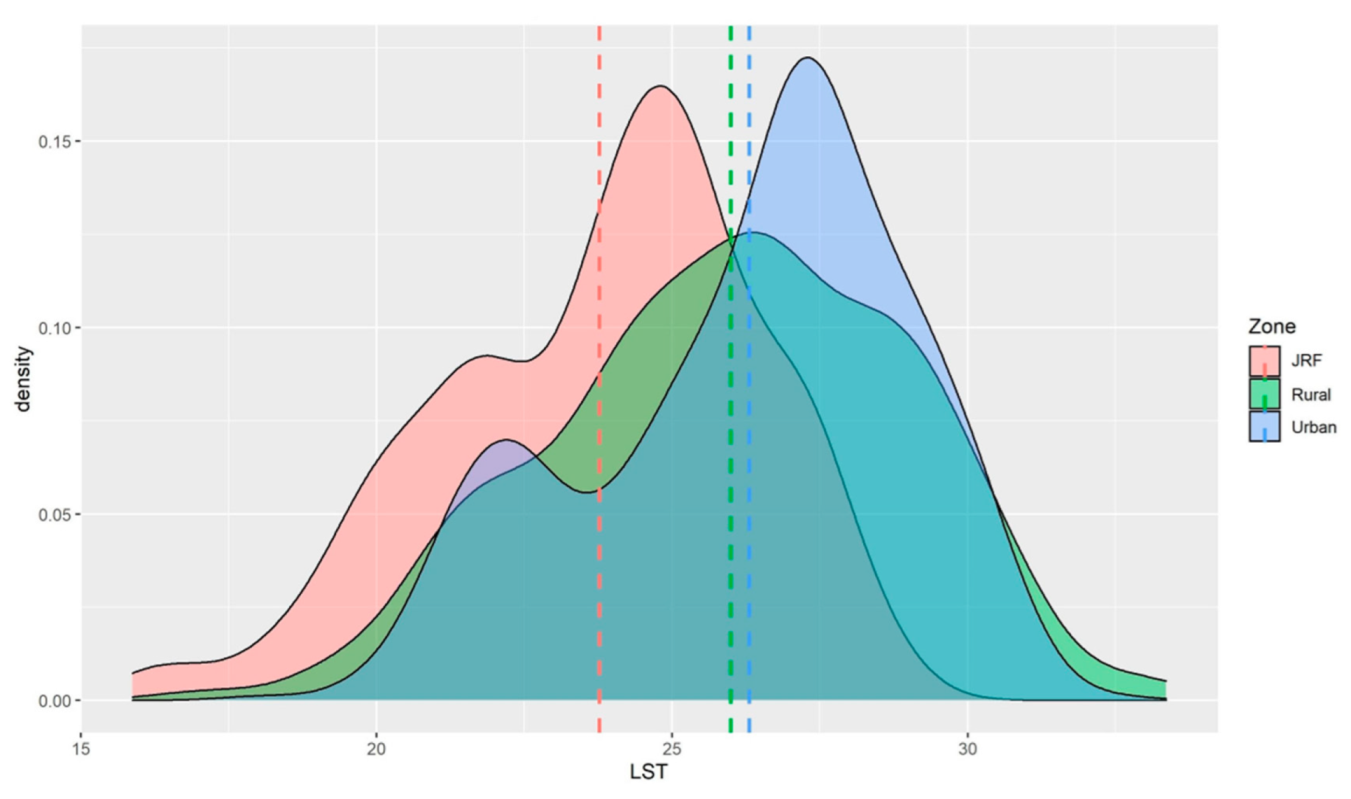
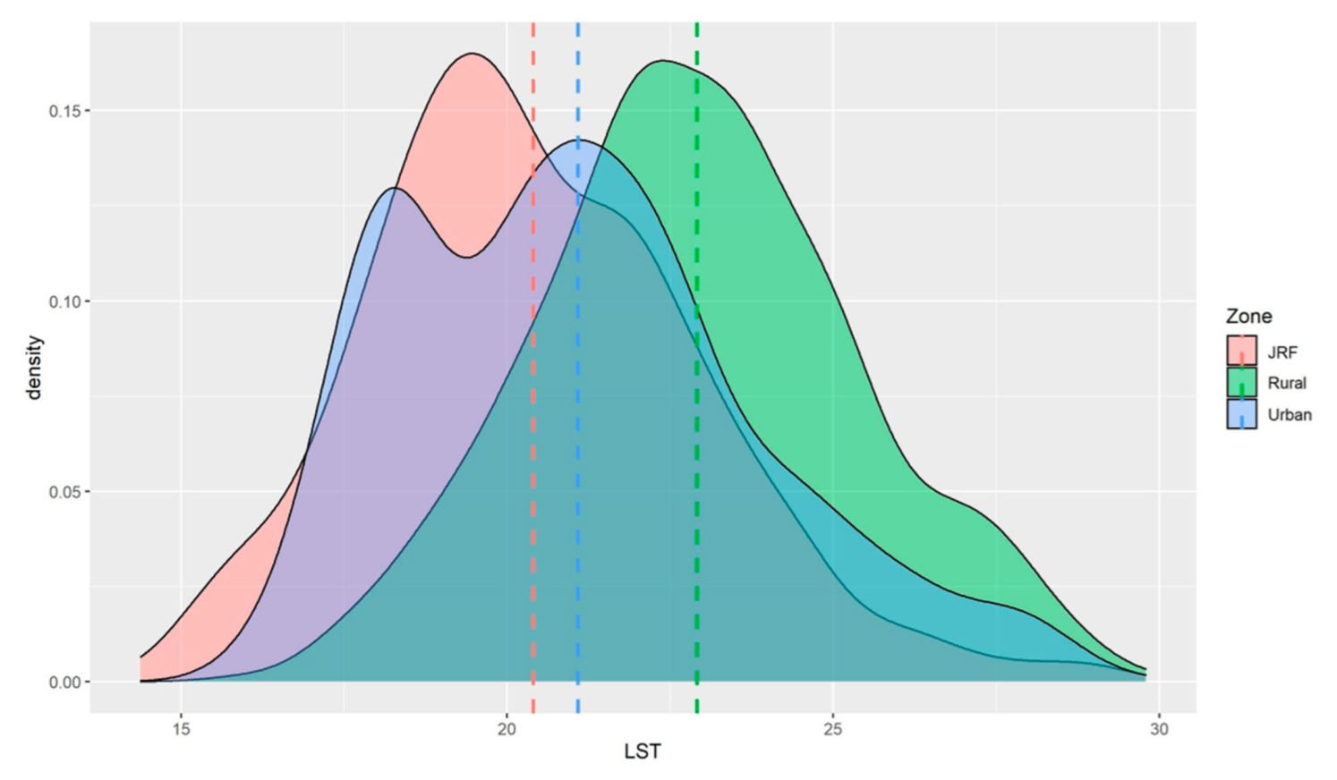
Cumulative zone-wise distribution of LSTs of the study zones was compared seasonally based on raster sampling points of all years included in the study. During the monsoon season, LSTs were highest in the urban areas (26.3 °C ± 2.6 SD), followed by the rural zone (25.9 °C ± 2.9 SD), and lowest in JRF (23.7 °C ± 2.6 SD; Figure 3).

Figure 3.
Zone-wise distribution of Land Surface Temperatures (°C) in the monsoon seasons. JRF denotes Jhalana Reserve Forest.
We found that rural and urban LSTs, although statistically significant (p < 0.01), were not as pronounced in the Monsoon season (p = 0.048; Figure 4) as in the summer or winter.
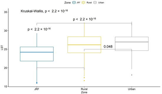
Figure 4.
Monsoon Zone-wise Land Surface Temperature variation and statistical significance.
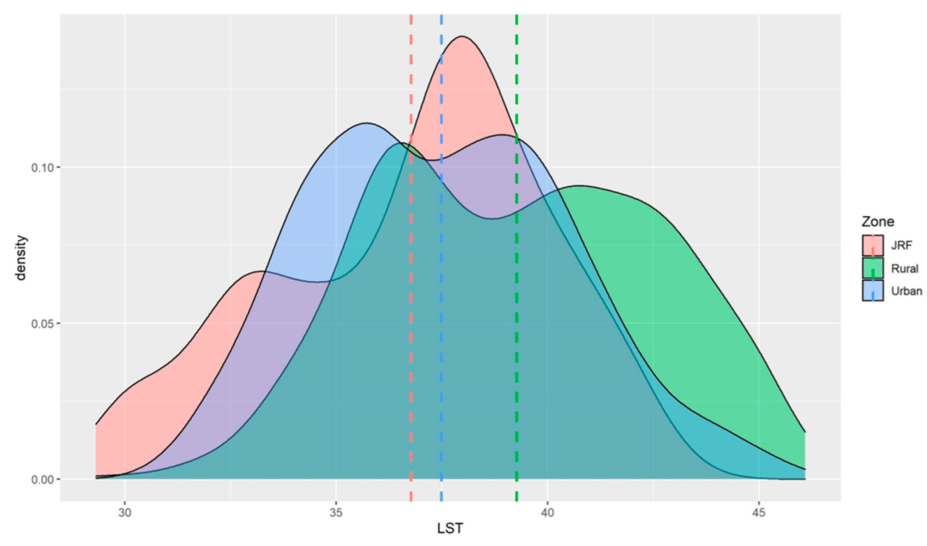
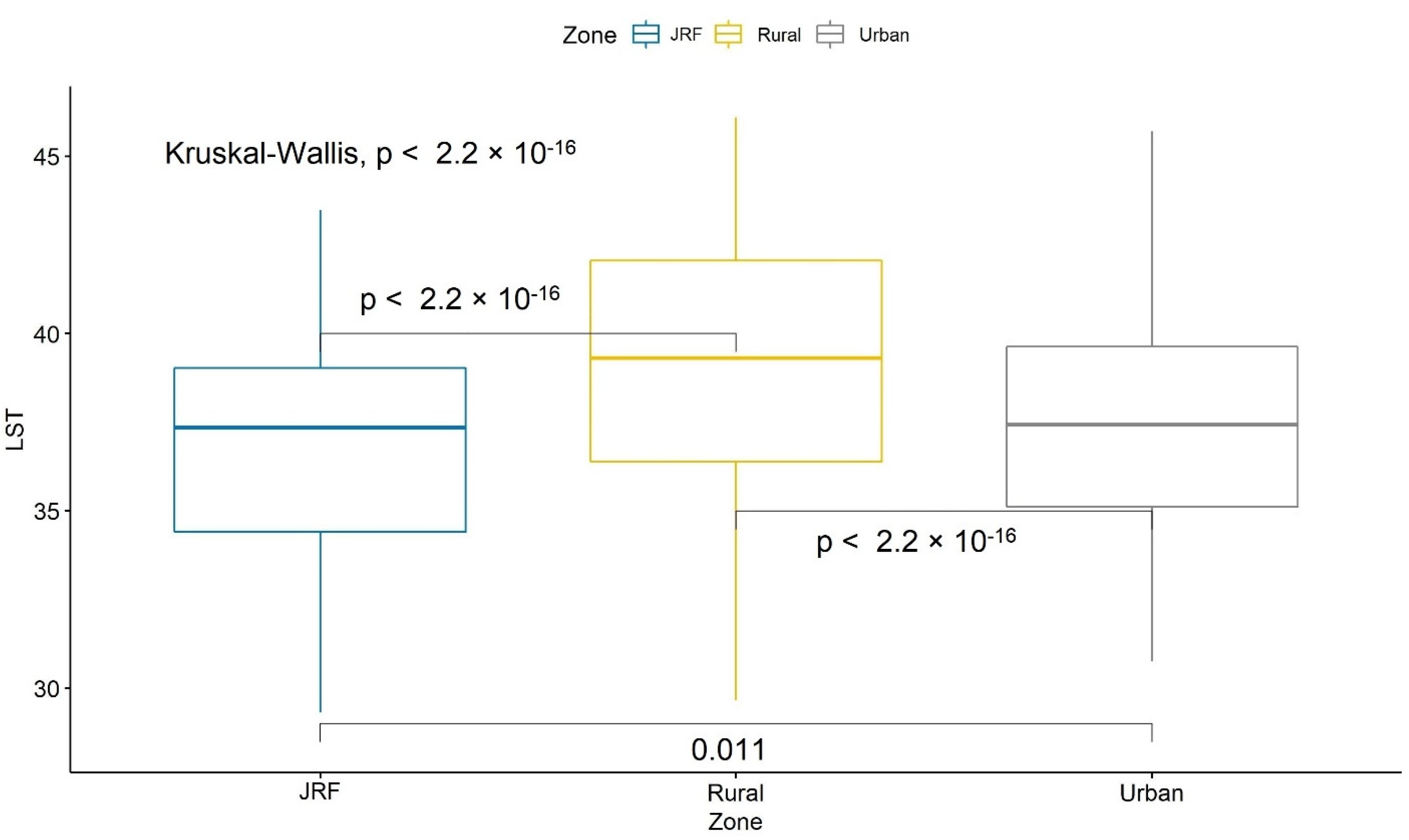
During the summer, LSTs of the rural zone were highest (39.2 °C ± 3.3 SD), the urban area was (37.4 °C ± 3.01 SD), and the lowest was the JRF (36.7 °C ± 3.2 SD; Figure 5).

Figure 5.
Zone-wise distribution of Land Surface Temperatures (°C) in the summer seasons.
In all three seasons and zone-wise comparisons, there were highly significant differences (p < 0.01) in LSTs, except for the rural zone in the summer, where it was slightly less (p = 0.011) than the highly statistically significant difference threshold (Figure 6).
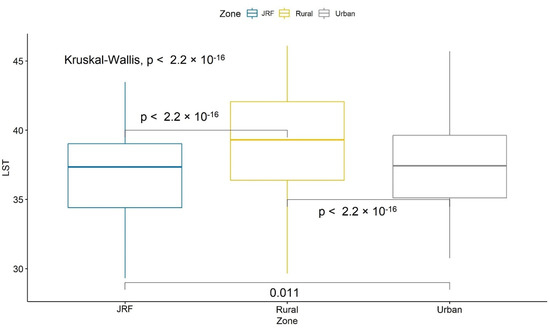
Figure 6.
Summer Zone-wise Land Surface Temperature variation and statistical significance among the urban and rural areas of Jaipur and the Jhalana Reserve Forest.
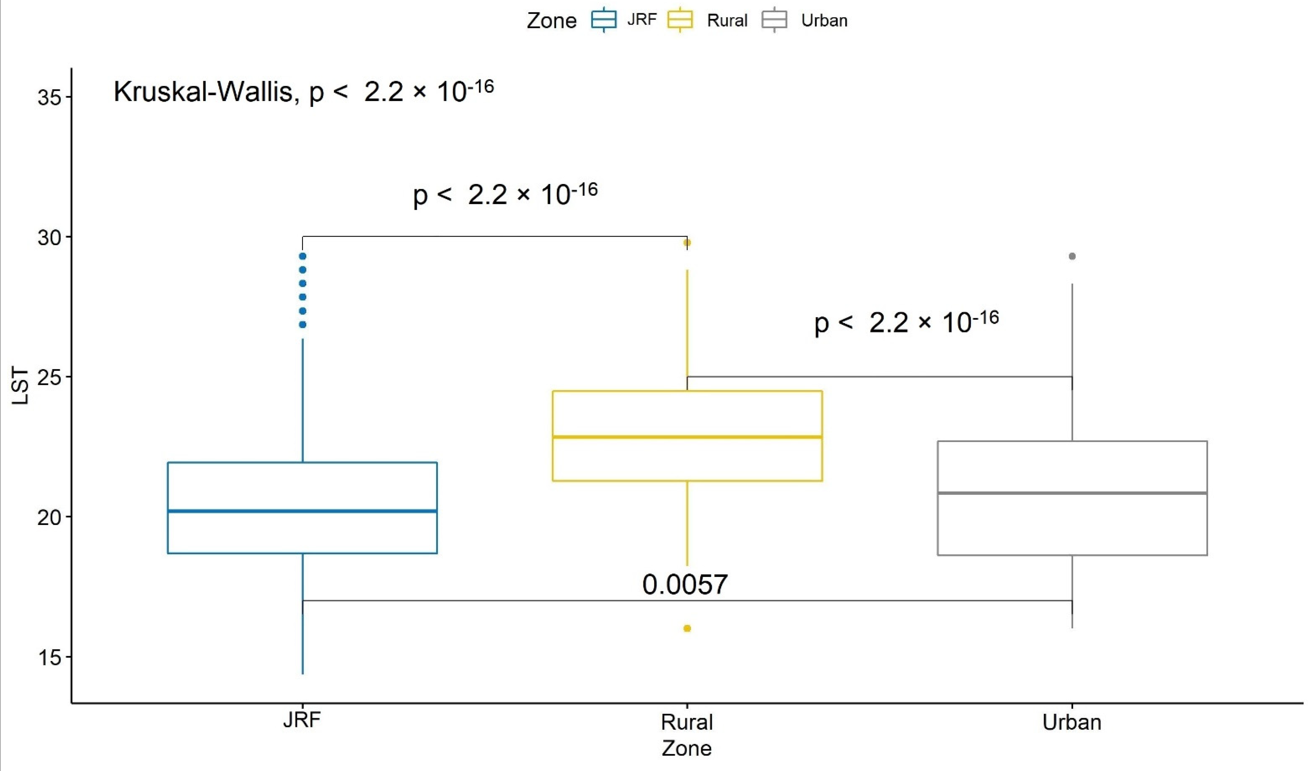
During the winter, LSTs of the rural areas (22.9 °C ± 2.4 SD) were usually higher than in the urban areas (21.08 °C ± 2.74 SD), and JRF was consistently the lowest (20.4 °C ± 2.55 SD; Figure 7).

Figure 7.
Zone-wise distribution of Land Surface Temperatures (°C) in the Winter seasons.
Winter zone-wise comparisons show the highest significant differences in LSTs between the three zones among all seasons (p < 0.01; Figure 8).
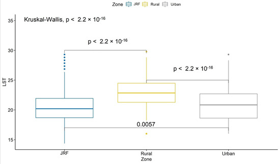
Figure 8.
Winter Zone-wise Land Surface Temperatures variation and statistical significance.
Thus, when observed seasonally, the mean LSTs were consistently lower for JRF throughout the year as compared to the urban and rural areas of the city of Jaipur.
3.2. Seasonal Analysis
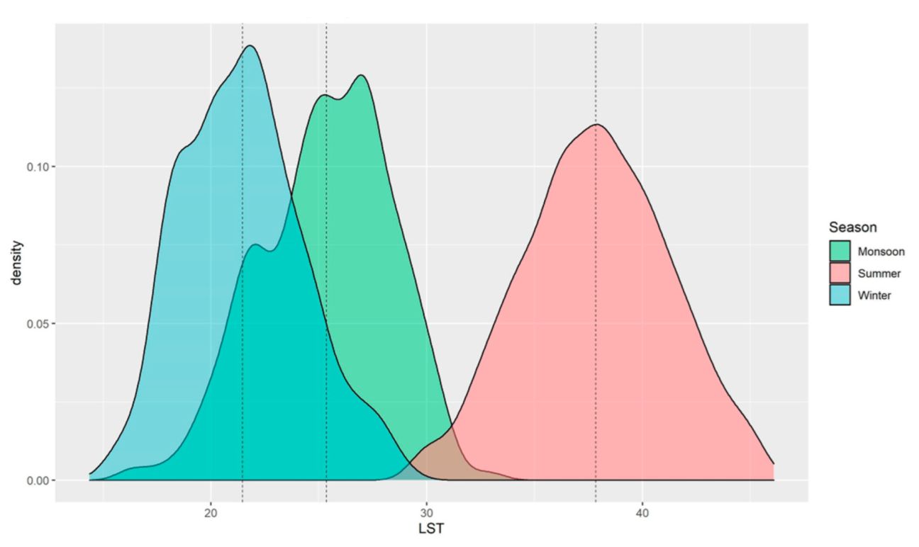
If season-wise LST distributions were considered exclusively, without zonal comparisons, it is clear that higher LSTs occur in the summer, followed by the monsoon season, and winter with significantly lower temperatures (Figure 9).

Figure 9.
Season-wise distribution of Land Surface Temperatures (°C) during the monsoon, summer, and winter seasons.
3.3. Demi-Decadal Analysis
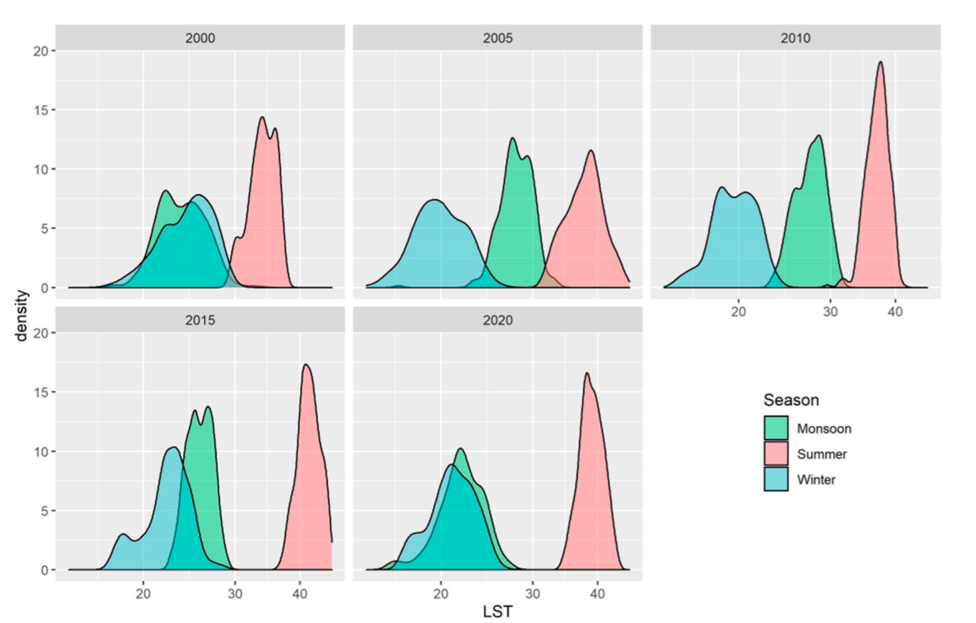
In a year-wise comparison of LSTs based on seasonal distributions, an ambiguity in LST distribution between Monsoon and Winter was observed only in the year 2000 (Figure 10).
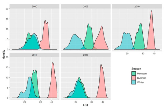
Figure 10.
Season-wise and year-wise distribution of Land Surface Temperatures (°C) during the monsoon, summer, and winter seasons.
To check for decadal differences, we compared the years 2000 and 2020 (Figure 7, Table 4). A significant increase of 4.8 °C in summer LSTs was observed as compared to decreases in the monsoon and winter seasons.
Table 4.
A comparison of the mean Land Surface Temperatures for the years 2000 and 2020.
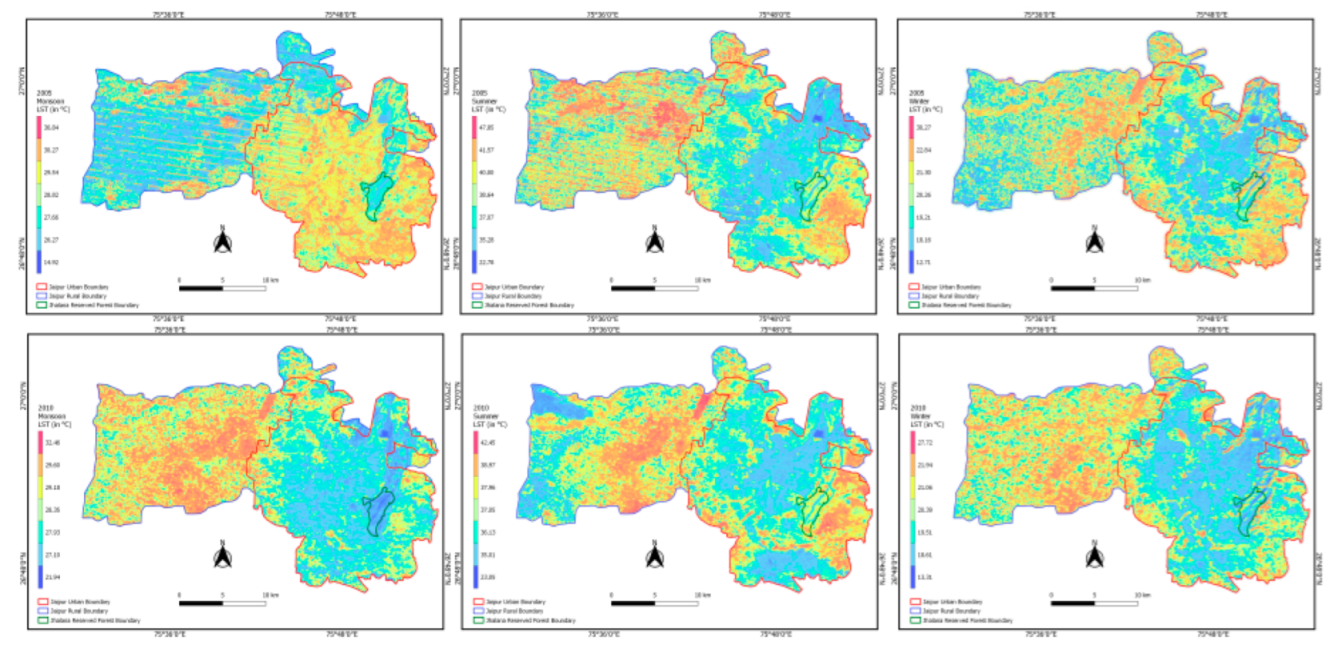
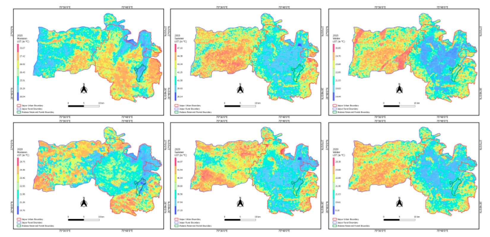
In addition, for visual comparison with maps, the series of maps show season-wise and year-wise LST maps (Figure 11, Figure 12 and Figure 13)
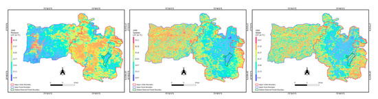
Figure 11.
Land Surface Temperature maps of the monsoon, summer, and winter seasons of the year 2000.
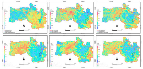
Figure 12.
Land Surface Temperature maps for the monsoon, summer, and winter seasons for the years 2005 (top row) and 2010 (bottom row).
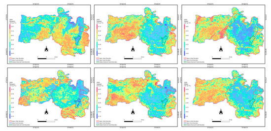
Figure 13.
Land Surface Temperature maps the monsoon, summer, and winter seasons for the years 2015 (top row) and 2020 (bottom row).
4. Discussion
Our study compared the LSTs of the urban and rural areas that encircle JRF. Our data show that in all three seasons, over the past two decades, the forested area in the midst of the urban and rural areas has the lowest LSTs. This suggests that the forest acts as a heat-sink regulating, i.e., decreasing the urban heat island (UHI) effect. In this case, the ecosystem services accorded by this “island” forest to the conurbation of Jaipur are impressive, especially in light of the fact that the summer LSTs have consistently increased over the past two decades resulting in much hotter summers with an increase of 4.8 °C.
Based on our results, the Urban Cool Island (UCI) effect is observed when the urban zone is considered, especially in summer and winter, whereas in JRF, an urban forest, UCI is observed in all three seasons. Thus, the urban zone and JRF together can be considered as components of the Urban Cool Island effects, where significantly lower LSTs are found across seasons compared to the rural zone. Several semi-arid climatic region cities with centralized vegetation areas demonstrate such UCI effects—in The UAE capital city of Abu Dhabi [20] and Ajmer in Rajasthan state in India [22].
Similarly, in Erbil, Iraq, on typical dry season days, during the daytime, the city center, which has an urban park, has significantly lower LSTs than the surrounding neighborhoods [21]. The same phenomenon was also observed in Raipur [17]. Similarly, the UCI effect was observed, especially in the winter and summer seasons for Jaipur. We assume that during the monsoon season, UCI effects are not observed because the surrounding barren land and agricultural areas are greener as compared to the other two seasons following the monsoon precipitation.
One of the reasons for this effect, sometimes referred to as the inversion of the UHI, includes the absence of vegetation, especially in rural agricultural croplands (uncultivated/fallow land) and large areas of barren land [42] during the winter and summer seasons. This was confirmed by our results in the monsoon LST distribution, where rural LSTs are also lower than in urban areas, which is possibly due to the presence of vegetation in the cultivated croplands and natural vegetation in areas that are barren outside the monsoon season.
In contrast, Urban areas exhibit lower LSTs in other seasons than rural surroundings since convection gets more efficient compared to rural areas containing bare soils mainly by the presence of trees and gardens and also by shade from buildings which reduces solar radiation in Urban areas [57].
Moreover, a study in Seoul, South Korea, shows that the mean LST of the urban forest was lower than the overall city’s mean LST and provided a cooling effect for the city [26]. Similarly, JRF shows lower LST throughout the study period as compared to the urban and rural zones of Jaipur city. JRF proves to be a heat sink for Jaipur, moderating the city from even higher ambient temperatures.
In addition, based on the LST observations, JRF provides a cooling effect and provides an important ecosystem service in spite of the warming trend observed in the summer for the past two decades. It is again confirmed in our study, as was found in multiple studies, that LSTs in urban areas in semi-arid/arid regions act as cool urban islands [21,58].
However, this phenomenon was not prominent in the monsoon season. We could not statistically confirm that a UHI effect is, in fact, present in monsoon because of the cooling effect of the rains on all the urban and rural areas. Additionally, during the monsoon, the fallow fields are green because of the growth of non-cultivated plants and weeds and which moderate the LST values cf. [33,34,35,36,37,38]. However, our personal observations need to be confirmed with data that JRF not only acts as a heat sink during the summer but also as a water sink. We have observed that during the monsoon rains, copious amounts of the run-off of the floods and rains in Jaipur are funneled into the forested area reducing damages to human habitation and infrastructure in the urban and rural areas.
Furthermore, it is important to state that JRF has significantly low LSTs compared to urban zones; thus, planning measures should focus not only on maintaining and conserving JRF but also on increasing tree cover in the surrounding buffer areas. Because Urban forests are important components of urban areas, since they provide multiple environmental and ecological services [59,60,61,62,63,64,65,66], one of the consistent environmental services is the cooling of the micro-climate, reducing the heat-stress evidenced worldwide in recent decades [7,63].
A minimum tree cover area of 15% in an urban area is considered to be the norm for the megacities of India). However, in the neighboring semi-arid state of Gujarat, many cities fall below this target with an average of 8.8% of tree–cover [67]. The only exceptions with Urban forests are Gandhinagar (Indroda park, 4.5 km2) and Bhavnagar (Victoria park having 2 km2) [61,62]. In comparison, JRF covers 10.75 km2, i.e., 53.9%.
The increase in overall mean LSTs by 4.8 °C in the summer during the study period resembles the global trend of increasing LSTs and subsequent heat waves. Hence, we recommend future planning measures to increase tree cover in buffer areas of urban forests, like JRF, to regulate LSTs, and enhance the standard of living of the human residents in the urban and rural areas.
5. Conclusions
We conclude that JRF contributes to the standard of living of the human residents of the conurbation of Jaipur by providing ecosystem services for the residents of Jaipur:
- The Urban Cooling effect in the urban and rural areas of Jaipur, i.e., JRF acting as a heat sink;
- Summer LSTs are on the rise based on our multi-decadal comparisons, but the relatively low LSTs in JRF remain constant in all of the seasons throughout the years;
- A significant difference in LST was observed among and between the three study zones, with JRF always being the lowest in all of the three seasons;
We recommend that future Urban Planning must include reserve forests or artificial plantations within urban areas and create “Urban Forests”.
Furthermore, if protected/reserve areas (mostly wildlife sanctuaries and forests) are present near a city, a buffer area should be created with increased tree cover such that the UHI effect is effectively decreased.
In order to increase the effectiveness of the urban cooling effect, it is preferable that trees are clumped to create green islands within the urban areas and which will provide more diverse ecosystem services, as has been identified in this study.
Author Contributions
Conceptualization, R.Y.; methodology, S.R. and A.B.; software, S.R. and A.B.; validation, A.B., S.K. and R.Y.; formal analysis, S.R. and A.B.; investigation, S.R. and A.B.; resources, R.Y.; data curation, S.R. and A.B.; writing—original draft preparation, A.B. and R.Y.; writing—review and editing, R.Y.; visualization, S.R.; supervision, A.M.; project administration, S.K. All authors have read and agreed to the published version of the manuscript.
Funding
This research received no external funding.
Data Availability Statement
Deposited at Mendeley https://data.mendeley.com//datasets/4p73sb9p2y/1 (accessed on 12 November 2021).
Conflicts of Interest
The authors declare no conflict of interest.
Abbreviations
LST(s) = Land Surface Temperature(s) (in °C); LULC = Land Use and Land Cover; UHI = Urban Heat Island; NDVI = Normalized Difference Vegetation Index; UCI = Urban Cool Island; JRF = Jhalana Reserve Forest; ASTER = Advanced Spaceborne Thermal Emission and Reflection Radiometer; MODIS = Moderate Resolution Imaging Spectroradiometer.
References
- Gogoi, P.P.; Vinoj, V.; Swain, D.; Roberts, G.; Dash, J.; Tripathy, S. Land use and land cover change effect on surface temperature over Eastern India. Sci. Rep. 2019, 9, 8859. [Google Scholar] [CrossRef] [PubMed]
- Rajeshwari, A.; Mani, N.D. Estimation of Land Surface Temperature of Dindigul District Using Landsat 8 Data. Int. J. Res. Eng. Technol. 2014, 3, 122–126. [Google Scholar] [CrossRef]
- Sahana, M.; Ahmed, R.; Sajjad, H. Analyzing land surface temperature distribution in response to land use/land cover change using split window algorithm and spectral radiance model in Sundarban Biosphere Reserve, India. Model. Earth Syst. Environ. 2016, 2, 81. [Google Scholar] [CrossRef]
- Gohain, K.J.; Mohammad, P.; Goswami, A. Assessing the impact of land use land cover changes on land surface temperature over Pune city, India. Quat. Int. 2021, 575–576, 259–269. [Google Scholar] [CrossRef]
- Witherick, M.; Ross, S.; Small, J. A Modern Dictionary of Geography, 4th ed.; Oxford University Press: Oxford, UK, 2001; ISBN 034080713X. [Google Scholar]
- Rasul, A.; Balzter, H.; Smith, C. Diurnal and Seasonal Variation of Surface Urban Cool and Heat Islands in the Semi-Arid City of Erbil, Iraq. Climate 2016, 4, 42. [Google Scholar] [CrossRef]
- Hou, H.; Estoque, R.C. Detecting Cooling Effect of Landscape from Composition and Configuration: An Urban Heat Island Study on Hangzhou. Urban For. Urban Green. 2020, 53, 126719. [Google Scholar] [CrossRef]
- Kolokotsa, D.; Psomas, A.; Karapidakis, E. Urban heat island in southern Europe: The case study of Hania, Crete. Sol. Energy 2009, 83, 1871–1883. [Google Scholar] [CrossRef]
- Peng, J.; Jia, J.; Liu, Y.; Li, H.; Wu, J. Seasonal contrast of the dominant factors for spatial distribution of land surface temperature in urban areas. Remote Sens. Environ. 2018, 215, 255–267. [Google Scholar] [CrossRef]
- Zhou, B.; Rybski, D.; Kropp, J.P. The role of city size and urban form in the surface urban heat island. Sci. Rep. 2017, 7, 4791. [Google Scholar] [CrossRef]
- Zhao, Z.Q.; He, B.J.; Li, L.G.; Wang, H.B.; Darko, A. Profile and concentric zonal analysis of relationships between land use/land cover and land surface temperature: Case study of Shenyang, China. Energy Build. 2017, 155, 282–295. [Google Scholar] [CrossRef]
- Peng, X.; Wu, W.; Zheng, Y.; Sun, J.; Hu, T.; Wang, P. Correlation analysis of land surface temperature and topographic elements in Hangzhou, China. Sci. Rep. 2020, 10, 10451. [Google Scholar] [CrossRef] [PubMed]
- Sarricolea, P.; Meseguer-Ruiz, O. Urban climates of large cities: Comparison of the urban heat Island effect in Latin America. In Urban Climates in Latin America; Springer: Cham, Switzerland, 2019; pp. 17–32. [Google Scholar] [CrossRef]
- Zhou, W.; Cao, F. Effects of changing spatial extent on the relationship between urban forest patterns and land surface temperature. Ecol. Indic. 2020, 109, 105778. [Google Scholar] [CrossRef]
- Mohan, M.; Kikegawa, Y.; Gurjar, B.R.; Bhati, S.; Kolli, N.R. Assessment of urban heat island effect for different land use-land cover from micrometeorological measurements and remote sensing data for megacity Delhi. Theor. Appl. Climatol. 2013, 112, 647–658. [Google Scholar] [CrossRef]
- Veena, K.; Parammasivam, K.M.; Venkatesh, T.N. Urban Heat Island studies: Current status in India and a comparison with the International studies. J. Earth Syst. Sci. 2020, 129, 85. [Google Scholar] [CrossRef]
- Guha, S.; Govil, H.; Dey, A.; Gill, N. A case study on the relationship between land surface temperature and land surface indices in Raipur City, India. Geogr. Tidsskr. Danish J. Geogr. 2020, 120, 35–50. [Google Scholar] [CrossRef]
- Shigeta, Y.; Ohashi, Y.; Tsukamoto, O. Urban Cool Island in Daytime-Analysis by Using Thermal Image and Air Temperature Measurements. In Proceedings of the Seventh International Conference on Urban Climate, Yokohama, Japan, 29 June–3 July 2009; pp. 3–6. [Google Scholar]
- Yang, C.; He, X.; Wang, R.; Yan, F.; Yu, L.; Bu, K.; Yang, J.; Chang, L.; Zhang, S. The Effect of Urban Green Spaces on the Urban Thermal Environment and Its Seasonal Variations. Forests 2017, 8, 153. [Google Scholar] [CrossRef]
- Lazzarini, M.; Marpu, P.R.; Ghedira, H. Temperature-land cover interactions: The inversion of urban heat island phenomenon in desert city areas. Remote Sens. Environ. 2013, 130, 136–152. [Google Scholar] [CrossRef]
- Rasul, A.; Balzter, H.; Smith, C. Spatial variation of the daytime Surface Urban Cool Island during the dry season in Erbil, Iraqi Kurdistan, from Landsat 8. Urban Clim. 2015, 14, 176–186. [Google Scholar] [CrossRef]
- Lakra, K.; Sharma, D. Geospatial Assessment of Urban Growth Dynamics and Land Surface Temperature in Ajmer Region, India. J. Indian Soc. Remote Sens. 2019, 47, 1073–1089. [Google Scholar] [CrossRef]
- Ekercin, S.; Orhan, O.; Dadaser-Celik, F. Investigating Land Surface Temperature Changes Using Landsat-5 Data and Real-Time Infrared Thermometer Measurements at Konya Closed Basin in Turkey. Int. J. Eng. Geosci. 2019, 4, 16–27. [Google Scholar] [CrossRef]
- Yang, Y.; Cao, C.; Pan, X.; Li, X.; Zhu, X. Downscaling land surface temperature in an arid area by using multiple remote sensingindices with random forest regression. Remote Sens. 2017, 9, 789. [Google Scholar] [CrossRef]
- Bindajam, A.A.; Mallick, J.; AlQadhi, S.; Singh, C.K.; Hang, H.T. Impacts of vegetation and topography on land surface temperature variability over the semi-arid mountain cities of Saudi Arabia. Atmosphere 2020, 11, 762. [Google Scholar] [CrossRef]
- Lee, P.S.H.; Park, J. An effect of urban forest on urban thermal environment in Seoul, South Korea, based on landsat imagery analysis. Forests 2020, 11, 630. [Google Scholar] [CrossRef]
- Bokaie, M.; Zarkesh, M.K.; Arasteh, P.D.; Hosseini, A. Assessment of Urban Heat Island based on the relationship between land surface temperature and Land Use/ Land Cover in Tehran. Sustain. Cities Soc. 2016, 23, 94–104. [Google Scholar] [CrossRef]
- Livesley, S.J.; McPherson, E.G.; Calfapietra, C. The Urban Forest and Ecosystem Services: Impacts on Urban Water, Heat, and Pollution Cycles at the Tree, Street, and City Scale. J. Environ. Qual. 2016, 45, 119–124. [Google Scholar] [CrossRef]
- Yao, L.; Li, T.; Xu, M.; Xu, Y. How the landscape features of urban green space impact seasonal land surface temperatures at a city-block-scale: An urban heat island study in Beijing, China. Urban For. Urban Green. 2020, 52, 126704. [Google Scholar] [CrossRef]
- Zhou, W.; Cao, F.; Wang, G. Effects of spatial pattern of forest vegetation on urban cooling in a compact megacity. Forests 2019, 10, 282. [Google Scholar] [CrossRef]
- Maimaitiyiming, M.; Ghulam, A.; Tiyip, T.; Pla, F.; Latorre-Carmona, P.; Halik, Ü.; Sawut, M.; Caetano, M. Effects of green space spatial pattern on land surface temperature: Implications for sustainable urban planning and climate change adaptation. ISPRS J. Photogramm. Remote Sens. 2014, 89, 59–66. [Google Scholar] [CrossRef]
- Kong, F.; Yin, H.; James, P.; Hutyra, L.R.; He, H.S. Effects of spatial pattern of greenspace on urban cooling in a large metropolitan area of eastern China. Landsc. Urban Plan. 2014, 128, 35–47. [Google Scholar] [CrossRef]
- Reyes, B.; Hogue, T.; Maxwell, R. Urban irrigation suppresses land surface temperature and changes the hydrologic regime in semi-arid regions. Water 2018, 10, 1563. [Google Scholar] [CrossRef]
- Liu, T.; Yu, L.; Zhang, S. Land Surface Temperature Response to Irrigated Paddy Field Expansion: A Case Study of Semi-arid Western Jilin Province, China. Sci. Rep. 2019, 9, 1563. [Google Scholar] [CrossRef] [PubMed]
- Kourdounouli, C.; Jönsson, A.M. Urban ecosystem conditions and ecosystem services–a comparison between large urban zones and city cores in the EU. J. Environ. Plan. Manag. 2020, 63, 798–817. [Google Scholar] [CrossRef]
- Marando, F.; Salvatori, E.; Sebastiani, A.; Fusaro, L.; Manes, F. Regulating Ecosystem Services and Green Infrastructure: Assessment of Urban Heat Island effect mitigation in the municipality of Rome, Italy. Ecol. Modell. 2019, 392, 92–102. [Google Scholar] [CrossRef]
- Bolund, P.; Hunhammar, S. ANALYSIS Ecosystem services in urban areas. Ecol. Econ. 1999, 29, 293–301. [Google Scholar] [CrossRef]
- Dobbs, C.; Escobedo, F.J.; Zipperer, W.C. A framework for developing urban forest ecosystem services and goods indicators. Landsc. Urban Plan. 2011, 99, 196–206. [Google Scholar] [CrossRef]
- Jaber, S.M.; Abu-Allaban, M.M. MODIS-based land surface temperature for climate variability and change research: The tale of a typical semi-arid to arid environment. Eur. J. Remote Sens. 2020, 53, 81–90. [Google Scholar] [CrossRef]
- Bala, R.; Prasad, R.; Pratap Yadav, V. A comparative analysis of day and night land surface temperature in two semi-arid cities using satellite images sampled in different seasons. Adv. Space Res. 2020, 66, 412–425. [Google Scholar] [CrossRef]
- Guha, S.; Govil, H.; Gill, N.; Dey, A. Analytical study on the relationship between land surface temperature and land use/land cover indices. Ann. GIS 2020, 26, 201–216. [Google Scholar] [CrossRef]
- Jaber, S.M. On the relationship between normalized difference vegetation index and land surface temperature: MODIS-based analysis in a semi-arid to arid environment. Geocarto Int. 2021, 36, 1117–1135. [Google Scholar] [CrossRef]
- Kumbhojkar, S.; Yosef, R.; Benedetti, Y.; Morelli, F. Human-Leopard (Panthera pardus fusca) Co-Existence in Jhalana Forest Reserve, India. Sustainability 2019, 11, 3912. [Google Scholar] [CrossRef]
- Kumbhojkar, S.; Yosef, R.; Mehta, A.; Rakholia, S. A Camera-Trap Home-Range Analysis of the Indian Leopard (Panthera pardus fusca) in Jaipur, India. Animals 2020, 10, 1600. [Google Scholar] [CrossRef] [PubMed]
- Sharma, B.K.; Kulshreshtha, S.; Rahmani, A.R. (Eds.) Faunal Heritage of Rajasthan, India: Conservation and Management of Vertebrates, 1st ed.; Springer: Cham, Switzerland, 2013; ISBN1 978-3-319-01344-2. ISBN2 978-3-319-01345-9. [Google Scholar]
- Sharma, K.P.; Upadhyaya, B.P. Phytosociology, primary production and nutrient retention in herbaceous vegetation of the forestry arboretum on the Aravalli hills at Jaipur. Trop. Ecol. 2002, 43, 325–335. [Google Scholar]
- Kumbhojkar, S.; Yosef, R.; Kosicki, J.Z.; Kwiatkowska, P.K.; Tryjanowski, P. Dependence of the leopard Panthera pardus fusca in Jaipur, India, on domestic animals. Oryx 2021, 55, 692–698. [Google Scholar] [CrossRef]
- Agarwal, R.; Rijhwani, S. Diversity of Economically Useful Wild Plants of Jhalana Forest, Jaipur. Int. J. Pharma Bio Sci. 2021, 11, 38–43. [Google Scholar] [CrossRef]
- Indian Meteorological Department. Climatological Tables of Observations in India, 1981–2010; Indian Meteorological Department: New Delhi, India, 2010; p. 893. [Google Scholar]
- Peel, M.C.; Finlayson, B.L.; McMahon, T.A. Updated world map of the Köppen-Geiger climate classification. Hydrol. Earth Syst. Sci. 2007, 11, 1633–1644. [Google Scholar] [CrossRef]
- Cristóbal, J.; Jiménez-Muñoz, J.C.; Sobrino, J.A.; Ninyerola, M.; Pons, X. Improvements in land surface temperature retrieval from the Landsat series thermal band using water vapor and air temperature. J. Geophys. Res. Atmos. 2009, 114, D08103. [Google Scholar] [CrossRef]
- Das, D.N.; Chakraborti, S.; Saha, G.; Banerjee, A.; Singh, D. Analysing the dynamic relationship of land surface temperature and landuse pattern: A city level analysis of two climatic regions in India. City Environ. Interact. 2020, 8, 100046. [Google Scholar] [CrossRef]
- Rozenstein, O.; Qin, Z.; Derimian, Y.; Karnieli, A. Derivation of land surface temperature for landsat-8 TIRS using a split window algorithm. Sensors 2014, 14, 5768–5780. [Google Scholar] [CrossRef]
- Mallick, J.; Bindajam, A.A.; AlQadhi, S.; Ahmed, M.; Hang, H.T.; Thanh, N.V. A comparison of four land surface temperature retrieval method using TERRA-ASTER satellite images in the semi-arid region of Saudi Arabia. Geocarto Int. 2020, 37, 1757–1781. [Google Scholar] [CrossRef]
- R Core Team. R: A Language and Environment for Statistical Computing; R Foundation for Statistical Computing: Vienna, Austria, 2020; p. 3. [Google Scholar]
- QGIS Development Team. QGIS Geographic Information System; QGIS: Gruet, Switzerland, 2021. [Google Scholar]
- Masoodian, S.A.; Montazeri, M. Quantifying of surface urban cool island in arid environments case study: Isfahan metropolis. Landsc. Ecol. Eng. 2021, 17, 147–156. [Google Scholar] [CrossRef]
- McPherson, E.G.; Nowak, D.; Heisler, G.; Grimmond, S.; Souch, C.; Grant, R.; Rowntree, R. Quantifying urban forest structure, function, and value: The Chicago Urban Forest Climate Project. Urban Ecosyst. 1997, 1, 49–61. [Google Scholar] [CrossRef]
- Dwyer, J.F.; Nowak, D.J. A national assessment of the urban forest: An overview. In Portland ‘99, Pioneering New Trails: Proceedings of the Society of American Foresters 1999 National Convention, Portland, OR, USA, 11–15 September 1999; Society of American Foresters: Washington, WA, USA, 2000; pp. 157–162. [Google Scholar]
- Fung, C.K.W.; Jim, C.Y. Microclimatic resilience of subtropical woodlands and urban-forest benefits. Urban For. Urban Green. 2019, 42, 100–112. [Google Scholar] [CrossRef]
- Gage, E.A.; Cooper, D.J. Urban forest structure and land cover composition effects on land surface temperature in a semi-arid suburban area. Urban For. Urban Green. 2017, 28, 28–35. [Google Scholar] [CrossRef]
- Martini, A.; Biondi, D.; Batista, A.C. Urban Forest Components Influencing Microclimate and Cooling Potential. Rev. Árvore 2017, 41, e410603. [Google Scholar] [CrossRef]
- Moss, J.L.; Doick, K.J.; Smith, S.; Shahrestani, M. Influence of evaporative cooling by urban forests on cooling demand in cities. Urban For. Urban Green. 2019, 37, 65–73. [Google Scholar] [CrossRef]
- Esperon-Rodriguez, M.; Power, S.A.; Tjoelker, M.G.; Beaumont, L.J.; Burley, H.; Caballero-Rodriguez, D.; Rymer, P.D. Assessing the vulnerability of Australia’s urban forests to climate extremes. Plants People Planet 2019, 1, 387–397. [Google Scholar] [CrossRef]
- Vieira, T.A.; Panagopoulos, T. Urban Forestry in Brazilian Amazonia. Sustainability 2020, 12, 3235. [Google Scholar] [CrossRef]
- Konijnendijk, C.C. A decade of urban forestry in Europe. For. Policy Econ. 2003, 5, 173–186. [Google Scholar] [CrossRef]
- Singh, H.S. Tree density and canopy cover in the urban areas in Gujarat, India. Curr. Sci. 2013, 104, 1294–1299. [Google Scholar]


Publisher’s Note: MDPI stays neutral with regard to jurisdictional claims in published maps and institutional affiliations. |
© 2022 by the authors. Licensee MDPI, Basel, Switzerland. This article is an open access article distributed under the terms and conditions of the Creative Commons Attribution (CC BY) license (https://creativecommons.org/licenses/by/4.0/).