
Patterns and Driving Factors of Diversity in the Shrub Community in Central and Southern China


Abstract
:1. Introduction
2. Materials and Methods
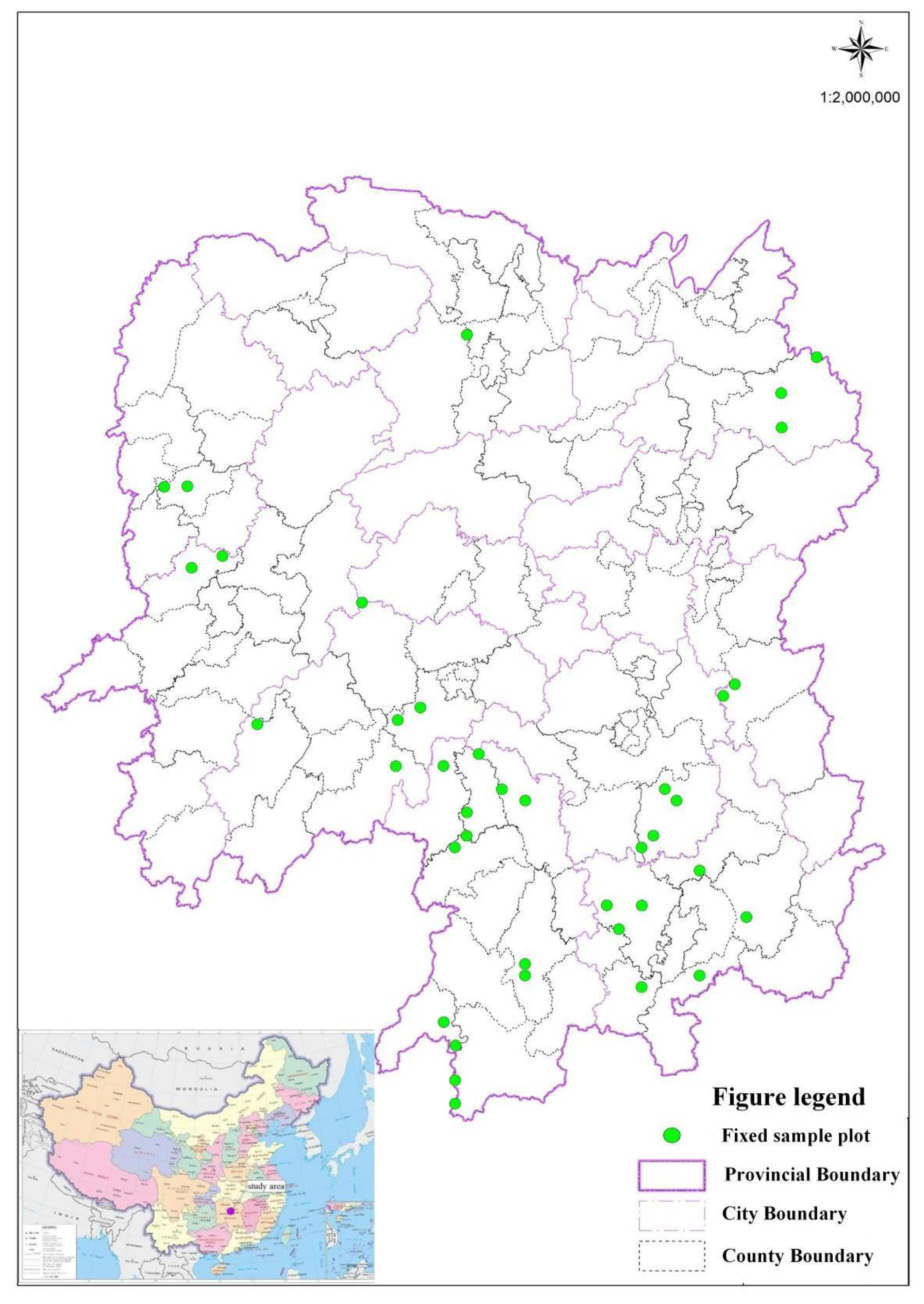
2.1. Data Sources
2.2. Species Diversity and Fitting of SAD
2.3. Prediction of Species Pool and Co-Occurrence Network
2.4. Detection of Driving Factors in Community Construction
3. Results
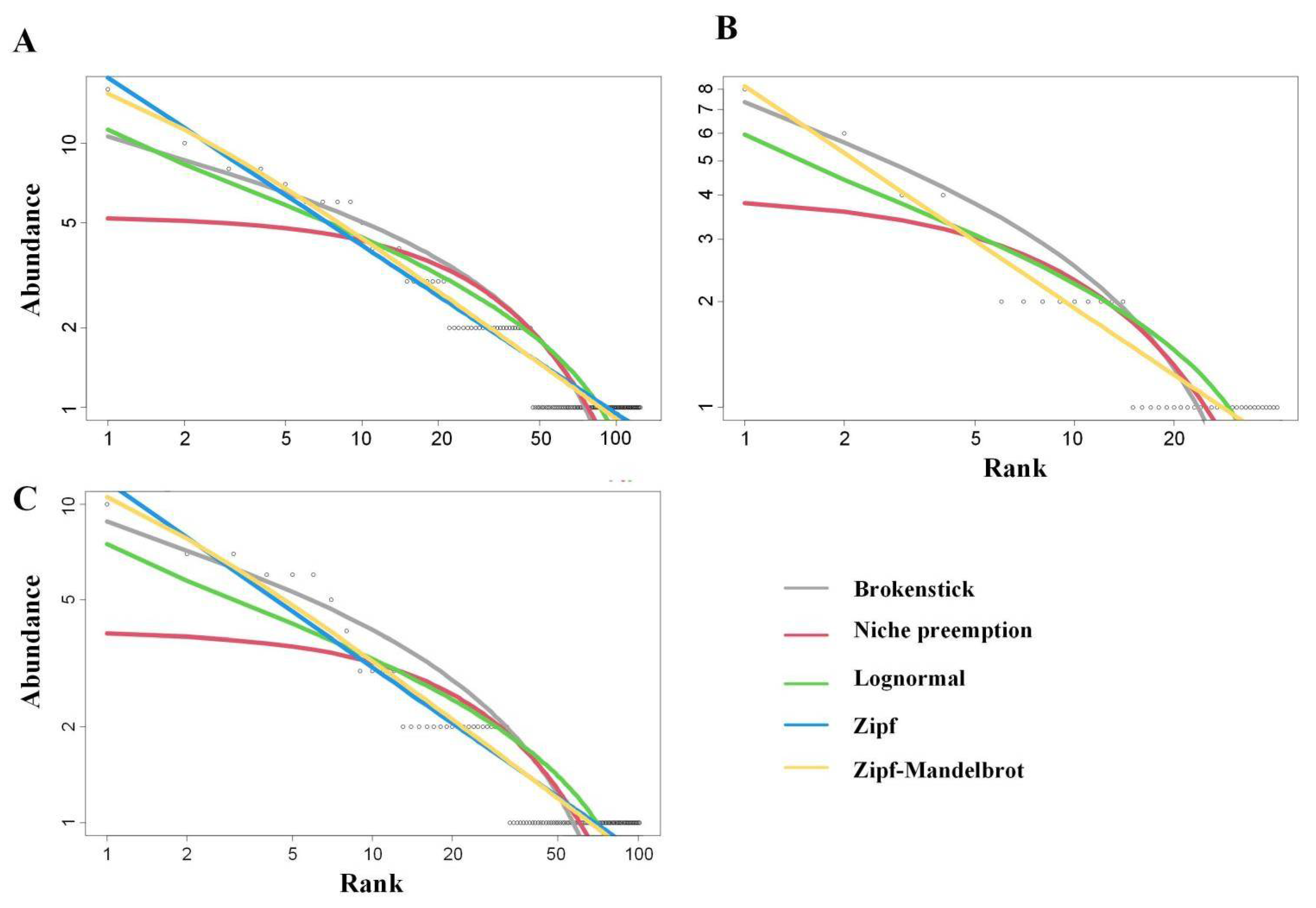
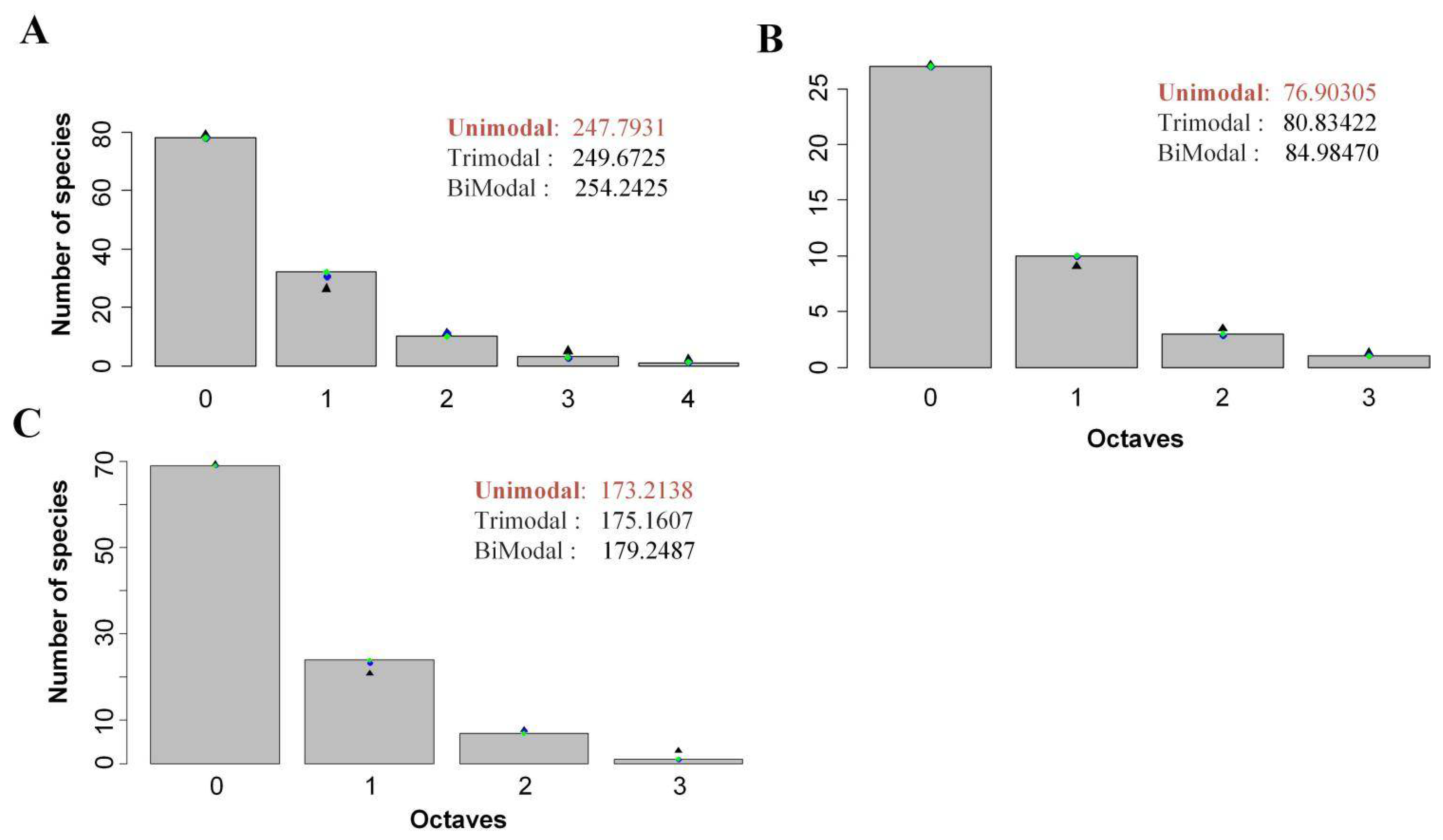
3.1. Fitting of SAD
3.2. Species Pool and Co-Occurrence Network
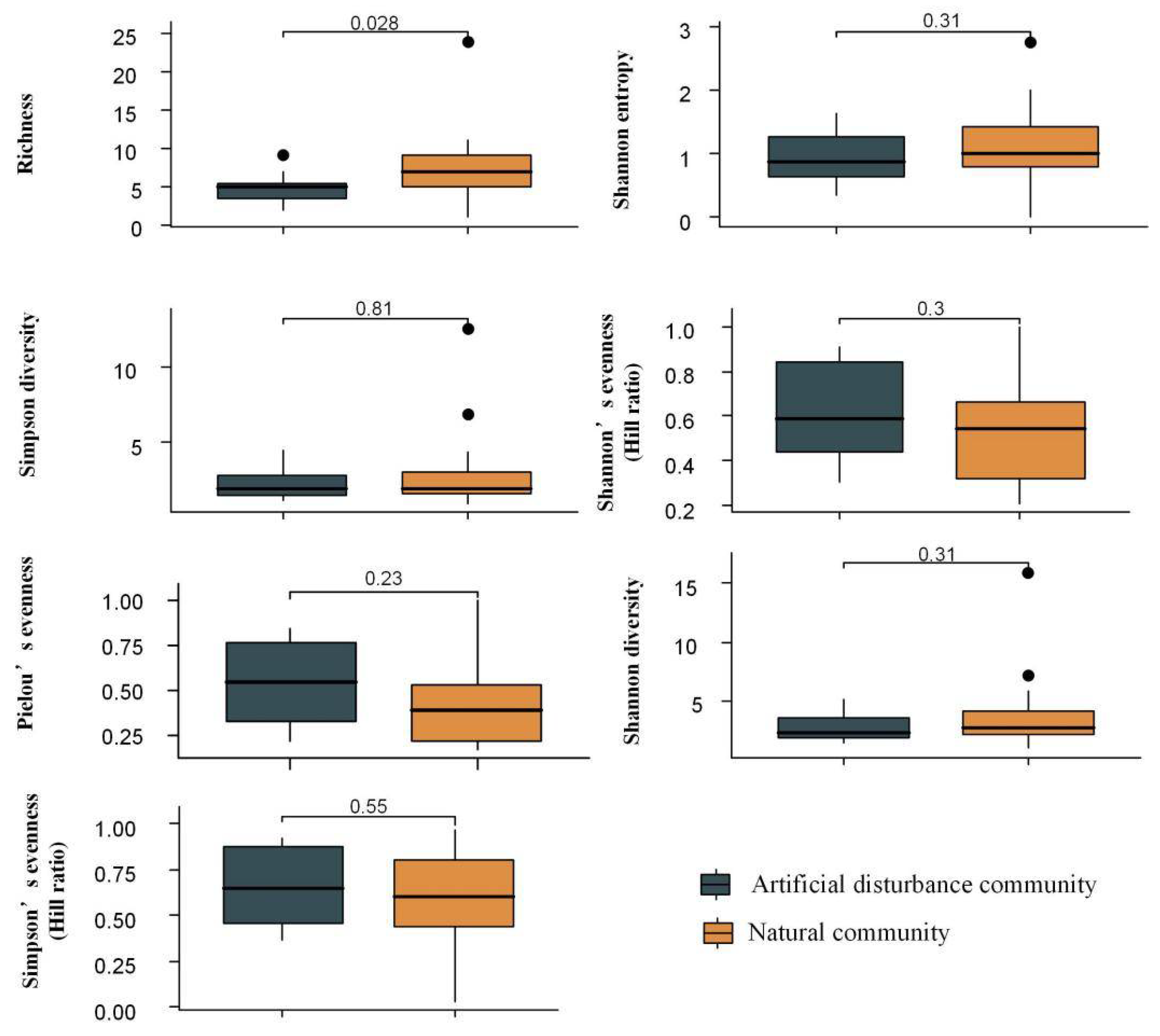
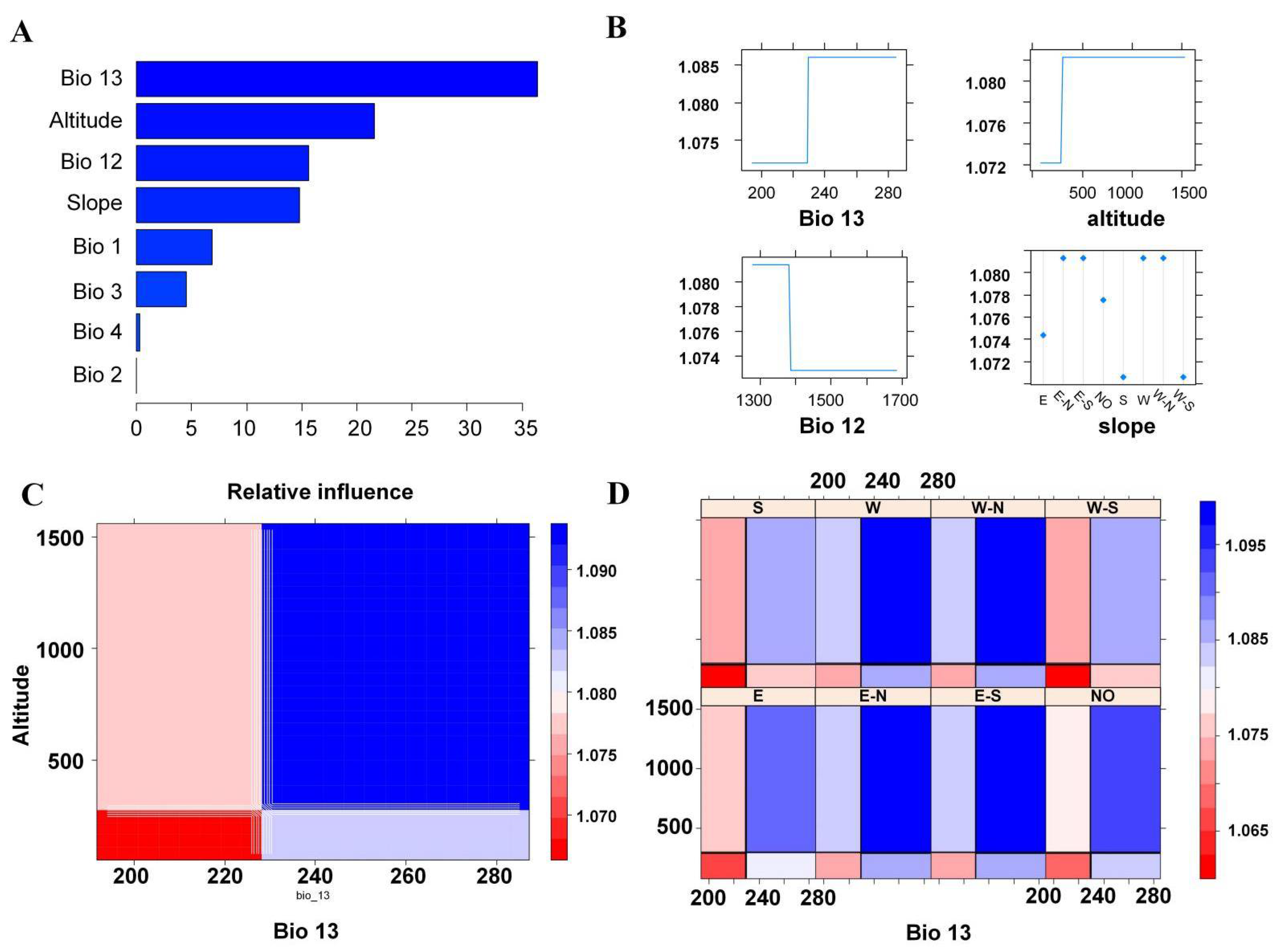
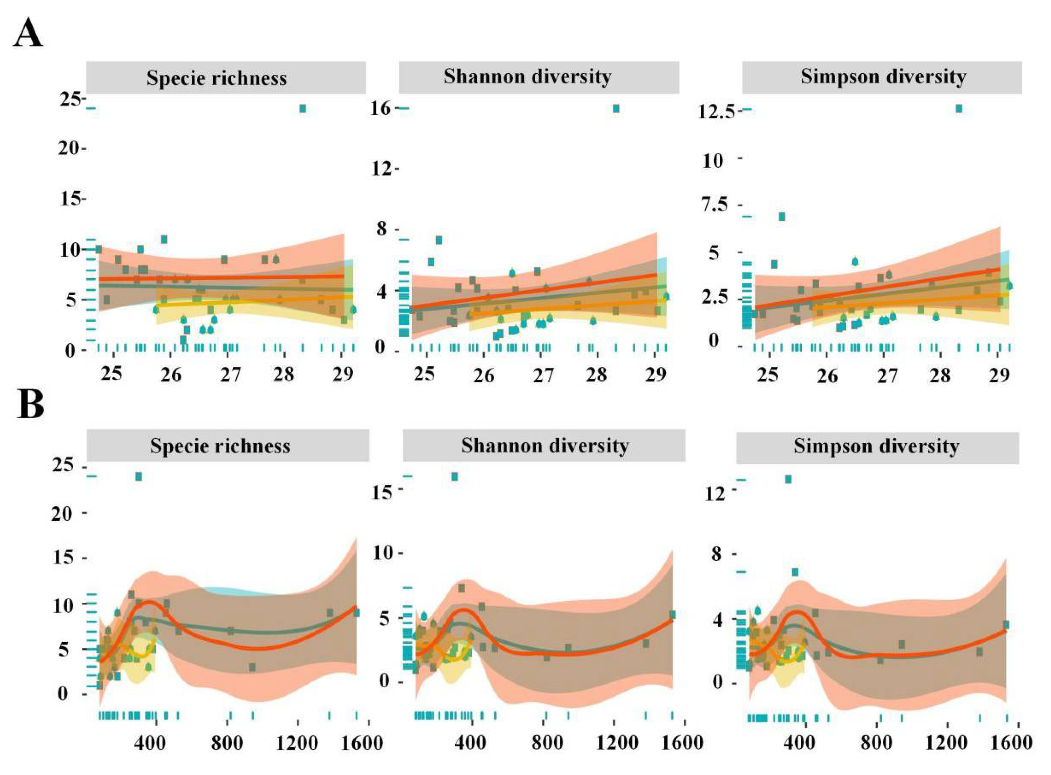
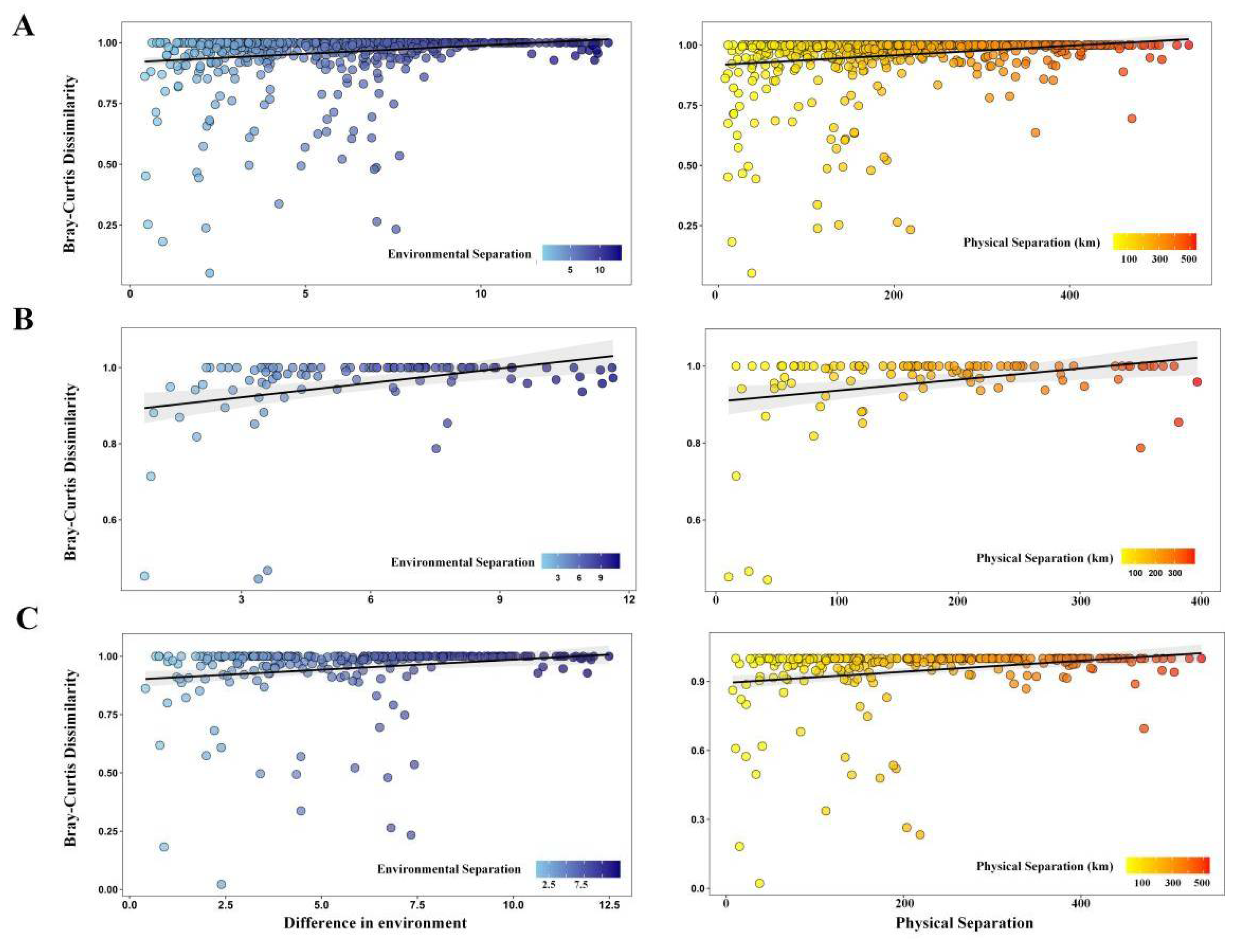
3.3. Driving Factors of Diversity
3.4. Indicator Species Based on MRT
3.5. Horizontal Distribution Pattern and Formation Mechanism of Diversity
4. Discussion
5. Conclusions
Supplementary Materials
Author Contributions
Funding
Institutional Review Board Statement
Informed Consent Statement
Acknowledgments
Conflicts of Interest
References
- Bormann, F.; Likens, G. An ecological study. Book reviews: Pattern and process in a forested ecosystem. Disturbance, development and the steady state based on the Hubbard brook ecosystem study. Science 1979, 205, 1369–1370. [Google Scholar]
- Gaston, K. Global patterns in biodiversity. Nature 2000, 405, 220–227. [Google Scholar] [CrossRef] [PubMed]
- Grytnes, J.; Vetaas, O. Species richness and altitude: A comparison between null models and interpolated plant species richness along the Himalayan altitudinal gradient. Nepal. Am. Nat. 2002, 159, 294–304. [Google Scholar] [CrossRef] [PubMed]
- Matthews, T.J.; Borregaard, M.K.; Gillespie, C.S.; Rigal, F.; Ugland, K.I.; Krüger, R.F.; Marques, R.; Sadler, J.P.; Borges, P.A.V.; Kubota, Y.; et al. Extension of the gambin model to multimodal species abundance distributions. Methods Ecol. Evol. 2019, 10, 432–437. [Google Scholar] [CrossRef] [Green Version]
- Wang, X.Z.; Ellwood, M.D.F.; Ai, D.; Zhang, R.; Wang, G. Species abundance distributions as a proxy for the niche-neutrality continuum. J. Plant Ecol. 2018, 11, 445–452. [Google Scholar] [CrossRef] [Green Version]
- Matthews, T.J.; Borges, P.A.V.; de Azevedo, E.B.; Whittaker, R.J. A biogeographical perspective on species abundance distributions: Recent advances and opportunities for future research. J. Biogeogr. 2017, 44, 1705–1710. [Google Scholar] [CrossRef]
- Hill, J.K.; Hamer, K.C. Using species abundance models as indicators of habitat disturbance in tropical forests. J. Appl. Ecol. 2002, 35, 458–460. [Google Scholar] [CrossRef]
- Chase, J.M. Towards a really unified theory for metacommunities. Funct. Ecol. 2005, 19, 182–186. [Google Scholar] [CrossRef]
- Sugihara, G.; Bersier, L.F.; Southwood, T.R.E.; Pimm, S.L.; May, R.M. Predicted correspondence between species abundances and dendrograms of niche similarities. Proc. Natl. Acad. Sci. USA 2003, 100, 5246–5251. [Google Scholar] [CrossRef] [Green Version]
- Wang, Z.; Fang, J.; Tang, Z.; Lin, X. Relative role of contemporary environment versus history in shaping diversity patterns of China’s woody plants. Ecography 2012, 35, 1124–1133. [Google Scholar] [CrossRef]
- Bernhardt-Roemermann, M.; Baeten, L.; Craven, D.; De Frenne, P.; Hedl, R.; Lenoir, J.; Bert, D.; Brunet, J.; Chudomelova, M.; Decocq, G.; et al. Drivers of temporal changes in temperate forest plant diversity vary across spatial scales. Glob. Chang. Biol. 2015, 21, 3726–3737. [Google Scholar] [CrossRef] [PubMed]
- Qian, H.; Jin, Y.; Ricklefs, R.E. Phylogenetic diversity anomaly in angiosperms between eastern Asia and eastern North America. Proc. Natl. Acad. Sci. USA 2017, 114, 11452–11457. [Google Scholar] [CrossRef] [PubMed] [Green Version]
- Večeřa, M.; Divíšek, J.; Lenoir, J.; Jiménez-Alfaro, B.; Biurrun, I.; Knollová, I.; Agrillo, E.; Campos, J.A.; Čarni, A.; Crespo Jiménez, G.; et al. Alpha diversity of vascular plants in European forests. J. Biogeogr. 2019, 46, 1919–1935. [Google Scholar] [CrossRef]
- Yeboah, D.; Chen, H. Diversity-disturbance relationship in forest landscapes. Landsc. Ecol. 2015, 31, 981–987. [Google Scholar] [CrossRef]
- van der Putten, W.H. Belowground drivers of plant diversity. Science 2017, 355, 134–135. [Google Scholar] [CrossRef]
- O’Brien, E.M. Biological relativity to water-energy dynamics. J. Biogeogr. 2006, 33, 1868–1888. [Google Scholar] [CrossRef]
- Xu, X.; Dimitrov, D.; Shrestha, N.; Rahbek, C.; Wang, Z. A consistent species richness-climate relationship for oaks across the northern hemisphere. Glob. Ecol. Biogeogr. 2019, 28, 1051–1066. [Google Scholar] [CrossRef]
- Seibold, S.; Bässler, C.; Brandl, R.; Büche, B.; Szallies, A.; Thorn, S.; Ulyshen, M.D.; Müller, J. Microclimate and habitat heterogeneity as the major drivers of beetle diversity in dead wood. J. Appl. Ecol. 2016, 53, 934–943. [Google Scholar] [CrossRef] [Green Version]
- Zilliox, C.; Gosselin, F. Tree species diversity and abundance as indicators of understory diversity in French mountain forests: Variations of the relationship in geographical and ecological space. For. Ecol. Manag. 2014, 321, 105–116. [Google Scholar] [CrossRef] [Green Version]
- Melo, F.P.; Arroyo-Rodríguez, V.; Fahrig, L.; Martínez-Ramos, M.; Tabarelli, M. In the hope for biodiversity-friendly tropical landscapes. Trends Ecol. Evol. 2013, 28, 462–468. [Google Scholar] [CrossRef]
- Barlow, J.; Gardner, T.A.; Louzada, J.; Peres, C.A. Measuring the conservation value of tropical primary forests: The effect of occasional species on estimates of biodiversity uniqueness. PLoS ONE 2010, 5, e9609. [Google Scholar] [CrossRef] [PubMed]
- Connell, J.H. Tropical rainforests and coral reefs as open non-equilibrium systems. In Population Dynamics; Blackwell: Oxford, UK, 1979; pp. 141–163. [Google Scholar]
- Van Gemerden, B.S.; Olff, H.; Parren, M.P.; Bongers, F. The pristine rain forest? Remnants of historical human impacts on current tree species composition and diversity. J. Biogeogr. 2003, 30, 1381–1390. [Google Scholar] [CrossRef]
- Chao, A.; Ricotta, C. Quantifying evenness and linking it to diversity, beta diversity, and similarity. Ecology 2019, 100, e02852. [Google Scholar] [CrossRef] [PubMed]
- Qin, H.; Dong, G.; Zhang, F. Relative roles of the replacement and richness difference components of beta diversity following the ecological restoration of a mountain meadow, north China. Ecol. Inform. 2019, 52, 159–165. [Google Scholar] [CrossRef]
- Socolar, J.B.; Gilroy, J.J.; Kunin, W.E.; Edwards, D.P. How should beta-diversity inform biodiversity conservation? Conservation targets at multiple spatial scales. Trends Ecol. Evol. 2016, 31, 67–80. [Google Scholar] [CrossRef] [Green Version]
- Ulrich, W.; Kusumoto, B.; Shiono, T.; Kubota, Y. Climatic and geographic correlates of global forest tree species–abundance distributions and community evenness. J. Veg. Sci. 2016, 27, 295–305. [Google Scholar] [CrossRef]
- Shukla, G.; Chakravarty, S. Fern diversity and biomass at Chilapatta Reserve forest of West Bengal Terai Duars in sub-humid tropical foothills of Indian Eastern Himalayas. J. For. Res. 2012, 23, 609–613. [Google Scholar] [CrossRef]
- Preston, F.W. The commonness and rarity of species. Ecology 1984, 29, 254–283. [Google Scholar] [CrossRef]
- Whittaker, R.H. Dominance and diversity in land plant communities. Science 1965, 147, 250–260. [Google Scholar] [CrossRef]
- Ugland, K.I.; Lambshead, P.J.D.; McGill, B.; Gary, J.S.; O’Dea, N.; Ladle, R.J.; Whittaker, R.J. Modelling dimensionality in species abundance distributions: Description and evaluation of the Gambin model. Evol. Ecol. Res. 2007, 9, 313–324. [Google Scholar]
- Chao, A. Estimating the population size for capture-recapture data with unequal catchability. Biometrics 1987, 43, 783–791. [Google Scholar] [CrossRef] [PubMed]
- Smith, E.P.; Belle, G.V. Nonparametric estimation of species richness. Biometrics 1984, 40, 119–129. [Google Scholar] [CrossRef] [Green Version]
- Chiu, C.H.; Wang, Y.T.; Walther, B.A.; Chao, A. An improved nonparametric lower bound of species richness via a modified Good-Turing frequency formula. Biometrics 2014, 70, 671–682. [Google Scholar] [CrossRef] [PubMed]
- De Cáceres, M.; Legendre, P.; Valencia, R.; Cao, M.; Chang, L.; Chuyong, G.; Condit, R.; Hao, Z.; Hsieh, C.; Hubbell, S.; et al. The variation of tree beta-diversity across a global network of forest plots. Glob. Ecol. Biogeogr. 2012, 21, 1191–1202. [Google Scholar] [CrossRef]
- De Cáceres, M.; Legendre, P.; Moretti, M. Improving indicator species analysis by combining groups of sites. Oikos 2010, 119, 1674–1684. [Google Scholar] [CrossRef]
- Peck, J.E. Multivariate Analysis for Community Ecologists: Step-by Step Using PC-ORD. Gleneden Beach: MjM Software Design. 2010. Available online: https://www.scienceopen.com/document?vid=ff3a0a0c-f1e9-4625-bb08-f2c975e246d5 (accessed on 1 December 2021).
- Chen, S.; Jiang, G.; Ouyang, Z.; Xu, W.; Xiao, Y. Relative importance of water, energy, and heterogeneity in determining regional pteridophyte and seed plant richness in China. J. Syst. Evol. 2011, 49, 95–107. [Google Scholar] [CrossRef]
- Gu, Y.; Han, S.; Zhang, J.H.; Chen, Z.J.; Wang, W.J.; Feng, Y.; Jiang, Y.J.; Geng, S.C. Temperature-dominated driving mechanisms of the plant diversity in temperate forests, Northeast China. Forests 2020, 11, 227. [Google Scholar] [CrossRef] [Green Version]
- Wright, S. Theory of path coefficients. Genetics 1923, 8, 239–255. [Google Scholar] [CrossRef]
- Frontier, S. Diversity and structure in aquatic ecosystems. Oceanogr. Mar. Biol. 1985, 23, 253–312. [Google Scholar]
- Volkov, I.; Banavar, J.R.; Hubbell, S.P.; Maritan, A. Neutral theory and relative species abundance in ecology. Nature 2003, 424, 1035–1037. [Google Scholar] [CrossRef] [Green Version]
- Ulrich, W.; Ollik, M.; Ugland, K.I. A meta-analysis of species-abundance distributions. Oikos 2010, 119, 1149–1155. [Google Scholar] [CrossRef]
- MacArthur, R.H. On the relative abundance of bird species. Proc. Nat. Acad. Sci. USA 1957, 43, 293–295. [Google Scholar] [CrossRef] [Green Version]
- Barange, M.; Campos, B. Models of species abundance: A critique of and an alternative to the dynamics model. Mar. Ecol. Prog. Ser. 1991, 69, 293–298. [Google Scholar] [CrossRef]
- Currie, D.J. Energy and Large-Scale Patterns of Animal- and Plant-Species Richness. Am. Nat. 1991, 137, 27–49. [Google Scholar] [CrossRef]
- Rahbek, C. The role of spatial scale and the perception of large-scale species-richness patterns. Ecol. Lett. 2005, 8, 224–239. [Google Scholar] [CrossRef]
- Zhang, Y.; Chen, H.Y.H.; Taylor, A. Multiple drivers of plant diversity in forest ecosystems. Glob. Ecol. Biogeogr. 2014, 23, 885–893. [Google Scholar] [CrossRef]
- Austrheim, G.; Eriksson, O. Plant species diversity and grazing in the Scandinavian mountains-patterns and processes at different spatial scales. Ecography 2001, 24, 683–695. [Google Scholar] [CrossRef]
- Moeslund, J.; Arge, L.; Bocher, P.; Dalgaard, T.; Svenning, J. Topography as a driver of local terrestrial vascular plant diversity patterns. Nord. J. Bot. 2013, 31, 129–144. [Google Scholar] [CrossRef]
- Alexander, J.M.; Kueffer, C.; Daehler, C.; Edwards, P.J.; Pauchard, A.; Seipel, T.; Arévalo, R.J.; Cavieres, L.A.; Dietz, H.; Jakobs, G.; et al. Assembly of nonnative floras along elevational gradients explained by directional ecological filtering. Proc. Natl. Acad. Sci. USA 2011, 108, 656–661. [Google Scholar] [CrossRef] [Green Version]
- Grime, J. Competitive exclusion in herbaceous vegetation. Nature 1973, 242, 344–347. [Google Scholar] [CrossRef]
- Connell, J. Diversity in tropical rain forests and coral reefs-High diversity of trees and corals is maintained only in a non-equilibrium state. Science 1978, 199, 1302–1310. [Google Scholar] [CrossRef] [PubMed] [Green Version]
- Mayor, S.J.; Cahill, J.F., Jr.; He, F.; Solymos, P.; Boutin, S. Regional boreal biodiversity peaks at intermediate human disturbance. Nat. Commun. 2012, 3, 1142. [Google Scholar] [CrossRef] [PubMed] [Green Version]
- Oommen, M.A.; Shanker, K. Elevational species richness patterns emerge from multiple local mechanisms in Himalayan woody plants. Ecology 2005, 86, 3039–3047. [Google Scholar] [CrossRef]
- Rahbek, C. The elevational gradient of species richness-A uniform pattern. Ecography 1995, 18, 200–205. [Google Scholar] [CrossRef]
- Zhang, J.; Zhang, M.; Mian, R. Effects of elevation and disturbance gradients on forest diversity in the Wulingshan Nature Reserve, North China. Environ. Earth Sci. 2016, 75, 904. [Google Scholar] [CrossRef]
- Syfert, M.; Brummitt, N.; Coomes, D.; Bystriakova, N.; Smith, M. Inferring diversity patterns along an elevation gradient from stacked SDMs: A case study on Mesoamerican ferns. Environ. Earth Sci. 2018, 16, e00433. [Google Scholar] [CrossRef]
- Zellweger, F.; Braunisch, V.; Morsdorf, F.; Baltensweiler, A.; Abegg, M.; Roth, T.; Bugmann, H.; Bollmann, K. Disentangling the effects of climate, topography, soil and vegetation on stand-scale species richness in temperate forests. For. Ecol. Manag. 2015, 349, 36–44. [Google Scholar] [CrossRef]
- Jocque, M.; Field, R.; Brendonck, L.; De Meester, L. Climatic control of dispersal-ecological specialization trade-offs: A metacommunity process at the heart of the latitudinal diversity gradient? Glob. Ecol. Biogeogr. 2010, 19, 244–252. [Google Scholar] [CrossRef]
- Yu, C.; Fan, C.; Zhang, C.; Zhao, X.; Gadow, K.V. Decomposing Spatial β-Diversity in the temperate forests of Northeastern China. Ecol. Evol. 2021, 11, 11362–11372. [Google Scholar] [CrossRef]
- Xing, D.; He, F.; Buckley, L. Environmental filtering explains a U-shape latitudinal pattern in regional β-deviation for eastern North American trees. Ecol. Lett. 2019, 22, 284–291. [Google Scholar] [CrossRef]


| Code | Description |
|---|---|
| Bio1 | Annual Mean Temperature |
| Bio2 | Mean Diurnal Range (Mean of monthly (max temp.–min temp.)) |
| Bio3 | Isothermality (BIO2/BIO7) (×100) |
| Bio4 | Temperature Seasonality (standard deviation ×100) |
| Bio5 | Max Temperature of Warmest Month |
| Bio6 | Min Temperature of Coldest Month |
| Bio7 | Temperature Annual Range (BIO5-BIO6) |
| Bio8 | Mean Temperature of Wettest Quarter |
| Bio9 | Mean Temperature of Driest Quarter |
| Bio10 | Mean Temperature of Warmest Quarter |
| Bio11 | Mean Temperature of Coldest Quarter |
| Bio12 | Annual Precipitation |
| Bio13 | Precipitation of Wettest Month |
| Bio14 | Precipitation of Driest Month |
| Bio15 | Precipitation Seasonality (Coefficient of Variation) |
| Bio16 | Precipitation of Wettest Quarter |
| Bio17 | Precipitation of Driest Quarter |
| Bio18 | Precipitation of Warmest Quarter |
| Bio19 | Precipitation of Coldest Quarter |
| Type | All Plots | ||||
|---|---|---|---|---|---|
| Model | M1 | M2 | M3 | M4 | M5 |
| Parameter 1 | / | 0.021363 | 0.38183 | 0.073054 | 0.096087 |
| Parameter 2 | / | / | 0.76961 | −0.63648 | −0.70504 |
| Parameter 3 | / | / | / | / | 0.80859 |
| Deviance | 69.0791 | 47.9878 | 24.3118 | 6.2648 | 5.5792 |
| AIC | 362.9997 | 343.9084 | 322.2324 | 304.1854 | 305.4998 |
| BIC | 362.9997 | 346.7287 | 327.873 | 309.8259 | 313.9607 |
| D statistic | 0.39516 | 0.37903 | 0.32258 | 0.3629 | 0.32258 |
| p-value of K-S test | 7.8 × 10⁻⁹ | 3.67 × 10⁻⁸ | 4.98 × 10⁻⁶ | 1.62 × 10⁻⁷ | 4.98 × 10⁻⁶ |
| Type | Artificial disturbance | ||||
| Model | M1 | M2 | M3 | M4 | M5 |
| Parameter 1 | / | 0.05423 | 0.33715 | 0.11671 | 0.11671 |
| Parameter 2 | / | / | 0.64207 | −0.63031 | −0.63032 |
| Parameter 3 | / | / | / | / | 3.37 × 10⁻⁵ |
| Deviance | 21.8428 | 11.1016 | 6.5021 | 1.7376 | 1.7376 |
| AIC | 116.4851 | 107.7438 | 105.1444 | 100.3798 | 102.3798 |
| BIC | 116.4851 | 109.4574 | 108.5715 | 103.807 | 107.5206 |
| D statistic | 0.43902 | 0.41463 | 0.36585 | 0.34146 | 0.34146 |
| p-value of K-S test | 0.0007397 | 0.001737 | 0.008274 | 0.01678 | 0.01678 |
| Type | Natural | ||||
| Model | M1 | M2 | M3 | M4 | M5 |
| Parameter 1 | / | 0.022811 | 0.32028 | 0.068435 | 0.084815 |
| Parameter 2 | / | / | 0.65743 | −0.58301 | −0.63843 |
| Parameter 3 | / | / | / | / | 0.66683 |
| Deviance | 60.4249 | 32.4401 | 18.8711 | 5.8502 | 5.5021 |
| AIC | 292.1572 | 266.1724 | 254.6034 | 241.5825 | 243.2344 |
| BIC | 292.1572 | 268.7876 | 259.8337 | 246.8127 | 251.0798 |
| D statistic | 0.44554 | 0.40594 | 0.36634 | 0.35644 | 0.35644 |
| p-value of K-S test | 3.92 × 10⁻⁹ | 1.18 × 10⁻⁷ | 2.60 × 10⁻⁶ | 5.35 × 10⁻⁶ | 5.35 × 10⁻⁶ |
| Model | Predicted Value | Variance |
|---|---|---|
| Observed species richness | 124 | - |
| Chao model | 243 | 37.44 |
| Jackknife model | 200 | 20.75 |
| Bootstrap model | 155 | 10.32 |
| Environment Distance | Environment Distance, Eliminate Geographic Distance | Geographic Distance | Geographic Distance, Eliminate Environment Distance | Type | |
|---|---|---|---|---|---|
| Statistic r | 0.1998 | 0.06522 | 0.2611 | 0.1522 | All |
| Significance | 0.0072 ** | 0.121 | 8.00 × 10⁻⁴ *** | 0.001 ** | |
| Statistic r | 0.2611 | 0.2434 | 0.2171 | 0.1564 | Artificial disturbance |
| Significance | 0.0115 * | 0.008 ** | 0.0678 | 0.099 | |
| Statistic r | 0.294 | 0.06308 | 0.3131 | 0.1672 | Natural |
| Significance | 0.0046 ** | 0.206 | 0.0016 ** | 0.015 * |
Publisher’s Note: MDPI stays neutral with regard to jurisdictional claims in published maps and institutional affiliations. |
© 2022 by the authors. Licensee MDPI, Basel, Switzerland. This article is an open access article distributed under the terms and conditions of the Creative Commons Attribution (CC BY) license (https://creativecommons.org/licenses/by/4.0/).
Share and Cite
Deng, N.; Song, Q.; Ma, F.; Tian, Y. Patterns and Driving Factors of Diversity in the Shrub Community in Central and Southern China. Forests 2022, 13, 1090. https://doi.org/10.3390/f13071090
Deng N, Song Q, Ma F, Tian Y. Patterns and Driving Factors of Diversity in the Shrub Community in Central and Southern China. Forests. 2022; 13(7):1090. https://doi.org/10.3390/f13071090
Chicago/Turabian StyleDeng, Nan, Qingan Song, Fengfeng Ma, and Yuxin Tian. 2022. "Patterns and Driving Factors of Diversity in the Shrub Community in Central and Southern China" Forests 13, no. 7: 1090. https://doi.org/10.3390/f13071090
APA StyleDeng, N., Song, Q., Ma, F., & Tian, Y. (2022). Patterns and Driving Factors of Diversity in the Shrub Community in Central and Southern China. Forests, 13(7), 1090. https://doi.org/10.3390/f13071090