Article

A Multistage Stochastic Program to Optimize Prescribed Burning Locations Using Random Fire Samples †

1
Faculty of Business and Economics, Phenikaa University, Yen Nghia, Ha Dong, Hanoi 12116, Vietnam
2
Department of Forest and Rangeland Stewardship, Colorado State University, Fort Collins, CO 80523, USA
*
Author to whom correspondence should be addressed.
This work was part of a dissertation of the corresponding author Dung Nguyen.
Forests 2022, 13(6), 930; https://doi.org/10.3390/f13060930
Submission received: 24 May 2022 / Revised: 13 June 2022 / Accepted: 13 June 2022 / Published: 14 June 2022
(This article belongs to the Section Natural Hazards and Risk Management)

Abstract

:
Selecting the optimal locations and timing for prescribed burning is challenging when considering uncertainties in weather, fire behavior, and future fire suppression. In this study, we present a sample average approximation (SAA) based multistage stochastic mixed integer program with recourse to optimize prescribed burning decisions. The recourse component of the SAA model considers post-fuel-treatment suppression decisions to manage fire spreads in multiple future planning periods. Our research aims at studying how an SAA model may benefit from using random fire samples to find good locations for prescribed burning during the first planning period. Two hypothetical test cases are designed to compare the impact of fire sample sizes on solution quality, and to illustrate how to identify high-quality period-one prescribed burning solutions. Results suggest that running SAA models using larger fire sample sizes can lead to better period-one solutions, but this benefit will diminish after the sample size reaches to certain thresholds. We found multiple period-one prescribed burning decisions that may result in similar effects in mitigating future wildfire risks.

1. Introduction

Wildfire is a natural component of many forest ecosystems. It has beneficial effects such as cleaning forest floor, restoring forest health, improving habitats and enhancing life cycles of fire-dependent forest species, but also posts threat to human life, properties, and natural resources [1,2,3]. During the past several decades, there has been escalation of extreme wildfire behaviors that led to increasing fire management costs. For example, the annual wildfire program spending for USDA Forest Service (USFS) and the Department of the Interior (DOI) increased from $2.3 billion in 2001 to $2.5 billion in 2005 [4]. Mitigating the negative impact from large detrimental fires is an important component of wildland fire management program.
An unintended consequence of aggressive fire suppression since the 20th century is the accumulation of forest fuels that consequently increases the risk of high intensity fires [5,6,7]. Fuel treatment represents a process of altering the quantity and structure of forest fuels [8,9]. It becomes increasingly important in wildfire management to change fire behaviors and reduce negative fire impacts [10,11,12,13,14,15,16,17,18,19,20,21,22]. For example, fuel treatment can slow fire spread [23], reduce fire intensity and severity [24,25], and potentially reduce fire sizes [26,27,28]. Fuel breaks created by treatments can also facilitate the establishment of fire control lines [9,29,30] and improve firefighter safety [31]. Commonly used fuel treatment methods include prescribed burning, mechanical thinning, and harvesting [32,33].
Both the amount and location of treatment impact its effectiveness. Some studies suggest treating around 20% of the total landscape areas to have a more consistent effect in reducing fire size and behavior [17,34,35]. If more areas are treated, fire size and behavior can be further decreased [17,36,37]. However, the marginal rate of reduction may diminish when the proportion of the landscape treated is beyond a threshold [17,34]. Treating an entire forest is often impractical [30,31,34,35,36,37,38,39,40,41,42] due to funding limits and potential conflicts with other management objectives (e.g., habitat protection or aesthetic concerns). The spatial arrangements of landscape fuel treatments also influence fire spread [43,44,45]. Research shows randomly located treatments are less effective in reducing fire spread [46] comparing to regular treatment patterns [17], especially if treatments can only be scheduled in a small fraction of a landscape [28,46,47]. Finney [9] suggests implementing treatments that overlap in the heading fire spread direction to reduce fire spread rate. Loehle [28] suggests fragmenting fuel complex by allocating treatments analogous to ship bulkhead. Palma et al. [48] suggests allocating treatments to disrupt critical fire spread paths. Other studies indicate that forming treatments as linear barriers [49] or parallel strips perpendicular to major fire spread directions [50,51] can effectively retard fire growth. It is also important for treatments to be spatially coordinated [10], as past research shows that fires, especially large and high intensity fires, can more easily circumvent uncoordinated treatment areas to travel through the landscape [38,39,40].
The effect of fuel treatment is often transient instead of permanent. The effectiveness of fuel treatments would decrease over time since fuel load would likely increase as tree and understory vegetation grows [6,52,53,54]. Therefore, periodically rescheduling fuel treatments on a landscape is often needed. This also increases the importance of fuel treatment planning to improve treatment efficiency and maintain treatment effectiveness across time and space [10,55]. Scheduling fuel treatments also requires careful consideration of management goals [56] and many other influencing factors [32,33,57]. Analytical tools, such as optimization models, can be used to support land managers in making better fuel treatment planning decisions.
Optimization models have been developed to configure spatial treatment layouts. Yemshanov et al. [58] used a network optimization model to find critical fuel treatment locations (i.e., nodes) that minimizes the chance of wildfires spreading through a landscape network. Hof et al. [59], and latterly Hof and Omi [60] developed mixed integer programming (MIP) models for scheduling treatments to delay the spread of a targeted fire from its ignition location to one or more targeted locations. Konoshima et al. [61] developed a dynamic programming model that can recognize numerous spread patterns and associated probabilities of a single fire and optimize fuel treatment and harvest based on those patterns in a hypothetical landscape. Wei et al. [62] developed a MIP model that uses a fire probability distribution map pre-calculated by simulating many random fires to optimize fuel treatment allocation to break fire probability accumulation paths. Wei [63] built another MIP model to schedule fuel treatment to provide control opportunities for a set of predicted future fires.
Some other optimization models were developed to locate fuel treatments to modify landscape fuel connectivity. Percolation theory [64,65] indicates that randomly treating a fraction of the landscape up to a “percolation threshold” could form connected fuel breaks to obstruct the spread of fires. Bevers et al. [26] used a shortest path network optimization model to discover that more than half of a forest would need to be treated to form continuous fuel breaks on most tested landscapes. Matsypura et al. [66] also used a network-based optimization technique to minimize the spatial connectivity of the landscape fuels. Their models considered the “graph connectivity measures” in the objective functions to minimize cell connectivity to reduce the potential of fire spread. Minas et al. [67] developed a MIP model to generate spatial fuel patterns to reduce the connectivity of “old fuel cells” in a landscape; the total number of connected pairs of “old fuel cells” is minimized across multiple periods to inhibit the spread of fires. Wei and Long [68] developed a spatial optimization model to fragment high fire hazard fuel patches to minimize the expected future fire losses weighted by the ignition probability of each fire. Post-optimization simulations suggest that scheduling fuel treatments to fragment fuel patches have similar effect as scheduling fuel treatments to slow the spread of long duration sample fires [68].
Selecting good fuel-treatment locations using optimization models remains challenging, mostly due to the complexities and uncertainties of wildfire problems [69]. Simulation models can handle complex and uncertain wildfire settings [70,71,72,73] to assist in making fuel treatment decisions, but using simulation alone cannot guarantee desired optimal outcomes. Thus, optimization-via-simulation were often implemented to find near-optimal solutions [74] in wildfire management [36,75,76,77,78]. For example, Finney et al. [35] integrated three models in a system: a forest and fuel dynamic model [79,80] to simulate forest vegetation changes over time, a spatially explicit model [51,78,81] to choose treatment locations, and a fire spread simulation model [81] to evaluate how treatments would modify fire growth rate, fire size, and conditional burn probability. Rytwinski and Crowe [82] ran a stochastic fire simulation model to compare fire risks of different fuel-break solutions identified by a meta-heuristic search algorithm [83]. González-Olabarria and Pukkala [36] used simulated annealing to iteratively search for better forest management strategies to maximize timber incomes and improve landscape fire resistance levels.
Fire suppression and fuel treatment often work jointly to mitigate fire risks [69]. Although fuel treatment alone may not stop fire spreads [46], it can improve the effectiveness of fire suppression effort [84]. Schaaf et al. [85] evaluated five combinations of fire suppression and fuel treatment programs on the Angeles National Forest in the western US and suggested that combining a low-intensity fire suppression program together with a moderate-intensity fuel treatment program would result in the highest return on investment. Mercer et al. [86] developed an integer programming model to evaluate tradeoffs between expenditures on fuels management and suppression. Another integer program was developed by Matthew et al. [87] to examine the cost-effectiveness of fuel treatments at multiple scales of investment to strengthen the nexus between fuel treatment and suppression response.
It is especially challenging to integrate fire behavior, fuel treatment, and fire suppression into one optimization model [88,89]. In this study, we developed and tested a novel multistage sample average approximation (SAA) program [90,91] to select prescribed burning locations in a landscape to minimize the expected loss from future wildfires. This SAA optimization program captures the spatial and temporal interactions of fire behaviors, prescribed burnings, and suppressions. So far, we have not found any other SAA program that can model those joint interactions. Since each model run is conducted based on a different set of random fire samples, it may suggest a different solution of prescribed fire layout. Repeatedly running the SAA program can generate a pool of solutions. Our second research objective is to design a heuristic method to select better quality prescribed burning layout solutions from those SAA generated solution candidates.

2. Materials and Methods

We introduce the general structure of the SAA program in Section 2.1. Its key components and major assumptions are described in Section 2.2, followed by the detailed SAA formulation presented in Section 2.3.

2.1. The Structure of the Stochastic Program

SAA is well-known method for building an approximate problem of a stochastic optimization problem [92]. By solving the approximate problem multiple times, it provides increasingly accurate solutions and also provides confidence intervals of the optimal objective function value that can be used to assess the quality of solutions [90,93]. More detailed characterization and properties of the SAA method could be found in the literature [93].
The stochastic program in this study follows the general structure of multistage stochastic program with recourse proposed by Birge and Louveaux [90,91]. It models prescribed burning and suppression decisions in multiple planning periods (or multiple stages) to mitigate risks from future wildfires. We use randomly sampled fires across the entire planning horizon to model the uncertainties in fire ignition, spread and intensity. The design of this program is illustrated in Figure 1 where fires and management activities are represented by multiple “decision-fire-sequence” (DFS) samples; each DFS sample is a series of prescribed burning decisions, random fire events, and fire suppression decisions across all planning periods. DFS samples are incorporated into a SAA formulation [90] with the objective to minimize the sum of average discounted management (prescribed fire and suppression) costs plus average discounted fire losses across all modeled planning periods. The design of this stochastic program ensures that prescribed burning decisions made in the first period (or stage) would be identical for all DFS samples. Our interest lies in the quality of the first period prescribed burning decisions that must be made before future uncertainties can be revealed. We maintain a constant number of DFS samples beyond the first period to limit the model size and reduce computing difficulty of solving this stochastic program.

2.2. Key Components and Major Assumptions of the Stochastic Program

We model fire behavior, fire management activities, and forest succession on a raster landscape within a multi-period planning horizon. Raster “cell” is the smallest map unit for modeling fire behavior, fire suppression, and forest growth (i.e., the growth of forest age). The same land is also delineated into multiple “stands”; each stand encloses one or multiple cells. Stand is the smallest management unit for making prescribed burning decisions.
Prescribed burning decisions (either “treat” or “no treat”) must be made for all stands at the beginning of each planning period. When a stand is selected for prescribed burning, all raster cells within the same stand are considered being treated. We assume treated cells would likely carry fires with lower intensity, and the treatment effects would last for certain periods.
Wildfires are modeled as uncertain events across the entire planning horizon. Each fire ignites at a random location (i.e., a random cell) and spreads for a random duration under the influence of a randomly selected wind direction and speed. Fire spread is modeled based on “cellular automaton” (CA), a commonly used method to model fire spread using certain transition rules between neighboring cells [94,95]. CA was applied in an abundant number of studies [95,96,97,98,99,100,101,102,103,104,105] to effectively capture the development of fire spread patterns with different complexity levels. In our SAA program, a fire may spread at different speeds and intensities in different cells. In cells where fire intensity is beyond a critical threshold, surface fire may reach the forest canopy and cause crown fire. In addition to prescribed burning, wildfire also consumes fuels and reduce future fire spread rate and intensity. The beneficial effects of wildfire may also last for certain periods.
Fire suppression is modeled as fire control effort in cells of having surface fires and is assumed to stop fire spreading in those cells. The SAA formulation can capture the assumed impacts of wildfire and prescribed burning in creating suppression opportunities to stop the spread of surface fires in recently burned or treated areas. Note that fire suppression is treated as a recourse decision in our SAA formulation and is not the focus of this program.
Forest age (or age-class) is assigned and tracked for every raster cell during the planning horizon. Upon entering the next period, age-class of the forest in a cell will be increased by one unless the age-class transition is interrupted by wildfires (Figure 2). We assume a crown fire can destroy all trees in the cells it burns and reset age-class of the forest in those cells to zero, while a surface fire can only cause partial damage to the burned cell and do not reset the forest age-class. In this program, we assume that the value of a forest is positively correlated with its age (i.e., an older forest is associated with a higher value to be protected).

2.3. General Mathematical Formulation

Notations including abbreviations, indices, parameters, sets, and variables used in the mathematical formulation are defined in Appendix A.1. We recommend referring to it to understand the details of the model’s objective function and constraints presented in Section 2.3.1, Section 2.3.2, Section 2.3.3 and Section 2.3.4.

2.3.1. Define Objective Function

The objective function minimizes the sum of average discounted prescribed burning costs, average discounted fire suppression costs, and average discounted fire losses across all DFS samples (Equation (1)):
1 N n ( f F T n + f S U P n + f F L n )

2.3.2. Model Fire Management Decisions

Equation (2) guarantees the same first-stage prescribed burning decision (FT1, Appendix A.1) to be applied for all DFS samples as required by the “non-anticipativity” property of a SAA program; in other word, FT1 needs to be made before the realization of any random future fire situations.
x w = 1 , a , n = x w = 1 , a , n n ,   n
Fire control can only be attempted in cells where fire line intensities are low enough that a surface fire could not transit into a crown fire under the influence of a modeled wind speed and direction (Equation (3)):
r ( w , i , n ) , c o ( w , i , n ) , c c C ^ A c t i v e ( w , i , n ) , i ,   n , w
Fire control in a cell is assumed to be succeed and able to save that cell from being burned under the modeled fire line intensity (Equation (4)):
d ( w , i , n ) , c + r ( w , i , n ) , c 1 c C ^ A c t i v e ( w , i , n ) ,   i ,   n , w
The minimum fire arrival time (MFAT, Appendix A.1) of a cell will be set to an arbitrarily selected value greater than the active fire spread duration to indicate successful fire control in that cell (Equation (5)):
t ( w , i , n ) , c ( H ( w , i , n ) + φ ) × r ( w , i , n ) , c   c ( C ^ A c t i v e ( w , i , n ) \ C ^ I g n i t i o n ( w , i , n ) ) , i , n , w

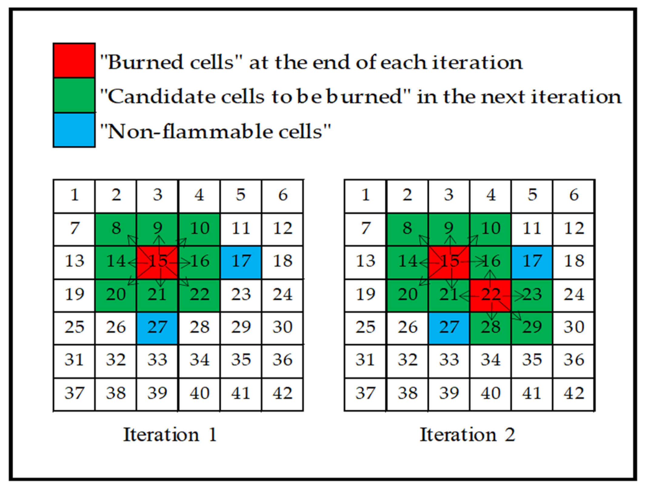
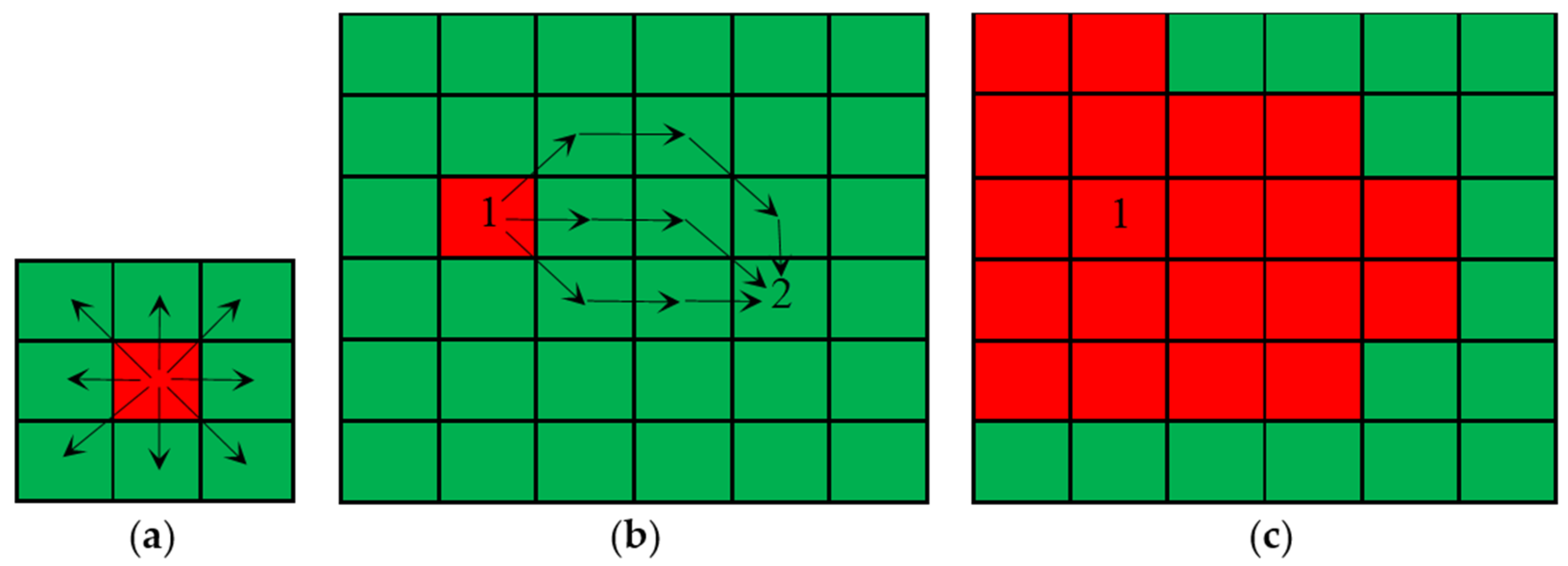
2.3.3. Model Wildfire Spread

Once started, fire is assumed to spread between adjacent cells along eight different directions (Figure 3a). A fire can spread from its ignition cell to any other cell in the rasterized landscape by following different “spread routes” (Figure 3b). Fire spread is modeled within a predefined maximum spread range (MSR, Figure 3c, Appendix A.2). The equations presented below can track all of the possible fire spread routes to a cell, and find the fastest route indicated by the MFAT of that cell. If the MFAT of a cell is less than the active fire spread duration, the cell will be considered “burned”. Throughout this paper, the term “burned” is only referred to wildfire to avoid confusion with prescribed burning.
Each fire starts at time zero from its ignition cell (Equation (6)) and will not burn non-flammable cells or cells lying outside its MSR (Equation (7)):
t ( w , i , n ) , c = 0   c = C ^ I g n i t i o n ( w , i , n ) , i , n , w
d ( w , i , n ) , c = 0 c C ^ I n A c t i v e ( w , i , n ) ,   i ,   n , w
A cell is considered as burned by a fire ( d ( w , i , n ) , c = 1 ) if that fire arrives the center of the cell within its predefined active fire spread duration (Equation (8)); otherwise, that cell is considered unburned ( d ( w , i , n ) , c = 0 and y ( w , i , n ) , c = 1 ) (Equations (9) and (10)):
d ( w , i , n ) , c H ( w , i , n ) t ( w , i , n ) , c M   c C ^ A c t i v e ( w , i , n ) ,   i ,   n , w
y ( w , i , n ) , c t ( w , i , n ) , c H ( w , i , n ) M     c C ^ A c t i v e ( w , i , n ) ,   i , n , w
d ( w , i , n ) , c + y ( w , i , n ) , c 1 c C ^ A c t i v e ( w , i , n ) ,   i ,   n , w
A cell must be burned if at least one of its adjacent cells was burned, unless fire control is applied in it, or fire cannot spread into it within the predefined active fire spread duration (Equation (11)):
d ( w , i , n ) , c + r ( w , i , n ) , c + y ( w , i , n ) , c d ( w , i , n ) , c c C ^ A c t i v e ( w , i , n ) , c C ^ c C ^ A c t i v e ( w , i , n ) ,   i ,   n , w
After a cell is burned, fire can spread from it to its adjacent cells (Equation (12)):
b ( w , i , n ) , c , c d ( w , i , n ) , c   c C ^ A c t i v e ( w , i , n ) , c C ^ c C ^ A c t i v e ( w , i , n ) ,   i , n , w
The potential of a fire traveling back after spreading from one cell to another is not allowed (Equation (13)):
b ( w , i , n ) , c , c + b ( w , i , n ) , c , c 1   c C ^ A c t i v e ( w , i , n ) , c C ^ c C ^ A c t i v e ( w , i , n ) ,   i , n , w
Equation (14) ensures that a non-ignition cell can only be burned by the fire spreading from exactly one of its adjacent cells. This equation also assumes that a fire will not spread back to its ignition cell.
c C ^ c C ^ A c t i v e ( w , i , n ) b ( w , i , , n ) , c , c = d ( w , i , n ) , c G ( w , i , n ) , c   c C ^ A c t i v e ( w , i , n ) ,   i ,   n , w
Equations (15) and (16) track whether the beneficial effects of prescribed burning or fires in the past would still exist in a cell at the time the sample fire ( w , i , n ) starts.
p ( w , i , n ) , c x w , a c , n + i < i d ( w , i , n ) , c + w W ^ w x w , a c , n + w W ^ w i d ( w , i , n ) , c c C ^ A c t i v e ( w , i , n ) , i ,   n , w
p ( w , i , n ) , c x w , a c , n + i < i d ( w , i , n ) , c + w W ^ w x w , a c , n + w W ^ w i d ( w , i , n ) , c M c C ^ A c t i v e ( w , i , n ) , i ,   n , w
The MFAT of each cell ( c ) is calculated by Equations (17) and (18) through tracking all of the possible spread paths from the adjacent cells ( c ) toward cell ( c ):
  • Equation (17) identifies the “upper bound” for the MFAT of cell c . Fire cannot arrive the center of cell c later than the MFAT of any of its adjacent cells ( c ) plus the spread time from the center of c to the center of c . If the fire does not burn cell c ( d ( w , i , n ) , c = 0 ) or if fire control effort is put in cell c ( r ( w , i , n ) , c = 1 ), the “Big M” will guarantee that the upper bound will not be set.
    t ( w , i , n ) , c t ( w , i , n ) , c + β c , c R O S ( w , i , n ) , c c × ( 1 p ( w , i , n ) , c ) + β c , c R O S ( w , i , n ) , c c × p ( w , i , n ) , c + β c , c R O S ( w , i , n ) , c c × ( 1 p ( w , i , n ) , c ) + β c , c R O S ( w , i , n ) , c c × p ( w , i , n ) , c + M × ( 1 d ( w , i , n ) , c + r ( w , i , n ) , c )   c ( C ^ A c t i v e ( w , i , n ) \ C ^ I g n i t i o n ( w , i , n ) ) ,   c C ^ c C ^ A c t i v e ( w , i , n ) ,   i , n , w
  • Equation (18) identifies the “lower bound” for the MFAT of cell c . Fire cannot arrive the center of cell c earlier than the MFAT of any of its adjacent cells ( c ) plus the spread time from the center of c to the center of c . If the fire cannot spread from c to c ( b w , a , c , c , n = 0 ), the “Big M” will guarantee that the lower bound will not be set.
    t ( w , i , n ) , c t ( w , i , n ) , c + β c , c R O S ( w , i , n ) , c c × ( 1 p ( w , i , n ) , c ) + β c , c R O S ( w , i , n ) , c c × p ( w , i , n ) , c + β c , c R O S ( w , i , n ) , c c × ( 1 p ( w , i , n ) , c ) + β c , c R O S ( w , i , n ) , c c × p ( w , i , n ) , c M × ( 1 b ( w , i , , n ) , c , c )   c ( C ^ A c t i v e ( w , i , n ) \ C ^ I g n i t i o n ( w , i , n ) ) ,   c C ^ c C ^ A c t i v e ( w , i , n ) ,   i , n , w
  • The exact MFAT of cell c can be identified when the upper bound and the lower bound are set and converged (equal values); Otherwise, the MFAT of cell c will be assigned a very large number to indicate fire would not burn that cell.
The fire line intensity in cell c is calculated based on the spread path that belongs to the fastest fire spread route (Equations (19)–(22)):
e ( w , i , n ) , c c C ^ c C ^ A c t i v e ( w , i , n ) b ( w , i , , n ) , c , c × E ( w , i , n ) , c c   c C ^ A c t i v e ( w , i , n ) ,   c C ^ c C ^ A c t i v e ( w , i , n ) ,   i , n , w
e ( w , i , n ) , c c C ^ c C ^ A c t i v e ( w , i , n ) b ( w , i , , n ) , c , c × E ( w , i , n ) , c c M × p ( w , i , n ) , c   c C ^ A c t i v e ( w , i , n ) ,   c C ^ c C ^ A c t i v e ( w , i , n ) ,   i , n , w
e ( w , i , n ) , c c C ^ c C ^ A c t i v e ( w , i , n ) b ( w , i , , n ) , c , c × E ( w , i , n ) , c c + M × ( 1 p ( w , i , n ) , c )   c C ^ A c t i v e ( w , i , n ) ,   c C ^ c C ^ A c t i v e ( w , i , n ) ,   i , n , w
Fire line intensity in cell c is compared to the critical threshold of fire line intensity in that same cell to decide whether the fire ( w , i , n ) would burn cell c at its current age-class as crown fire ( o ( w , i , n ) , c = 0 and e ( w , i , n ) , c j E c r i t i c a l ( w , i , n ) , c , j × q ( w , i , n ) , c , j ), or as surface fire ( o ( w , i , n ) , c = 1 and 0 < e ( w , i , n ) , c < j E c r i t i c a l ( w , i , n ) , c , j × q ( w , i , n ) , c , j ), or it would not burn cell c ( o ( w , i , n ) , c = 1 and e ( w , i , n ) , c = 0 ) (Equations (23) and (24)).
o ( w , i , n ) , c j E c r i t i c a l ( w , i , n ) , c , j × q ( w , i , n ) , c , j e ( w , i , n ) , c M   c C ^ A c t i v e ( w , i , n ) ,   i ,   n , w
1 o ( w , i , n ) , c e ( w , i , n ) , c j E c r i t i c a l ( w , i , n ) , c , j × q ( w , i , n ) , c , j M     c C ^ A c t i v e ( w , i , n ) ,   i , n , w

2.3.4. Estimate Fire Damages and Consequences of Prescribed Burning and Fire Suppression

Prescribed burning decisions are made for each stand instead of cell. The cost of treating a stand is the total costs of treating all cells within it. Treatment cost decreases in previously treated or burned cells (Appendix A.3, Equations (A1)–(A5)). For each DFS, the discounted total cost of prescribed burning in each period is calculated by Equation (25), and is constrained to be non-increasing between consecutive periods (Equation (26)). This management rule helps more evenly distribute treatment workload across time.
a A ^ 1 ( 1 + R ) L w × ( P F T × C a × x w , a , n ( P F T P F T ) × s w , a , n ) = f F T w , n n
f F T w , n f F T w 1 , n 0 n , w 2
The total discounted cost of prescribed burning across all planning periods is calculated for each DFS as in Equation (27).
w f F T w , n = f F T n n
The total discounted cost of fire control efforts through all planning periods is calculated for each DFS as in Equation (28).
w i c C ^ A c t i v e ( w , i , n ) 1 ( 1 + R ) L ( w , i , n ) × P S U P c × r ( w , i , n ) , c = f S U P n n
A set of book-keeping variables and constraints are used to identify the exact forest age-class and fire type in each cell when a fire occurs (Appendix A.3, Equations (A6)–(A16)). Fire loss in each cell can then be estimated based on both fire damage (associated with fire type) and forest value (associated with forest age class). For each DFS, the total discounted fire loss is calculated by Equation (29).
w i c C ^ A c t i v e ( w , i , n ) j 1 ( 1 + R ) L ( w , i , n )   × ( V ( w , i , n ) , c , j × v S u r f a c e ( w , i , n ) , c , j + V c , j × v C r o w n ( w , i , n ) , c , j ) = f F L n n

3. Test Cases

3.1. Testing Landscape and Assumptions

A synthesized landscape was used to test the SAA program. The landscape is consisted of 64 raster cells with side length of 150 m for each cell. It is manually delineated into 12 stands covered by forests (Figure 4). The landscape also includes non-flammable areas (i.e., open water with Stand-ID = 0). More detailed information of this landscape is presented in Appendix A.4.
All test cases assumed three ten-year planning periods. In each period, zero to multiple randomly generated fires might occur. Random numbers were drawn to determine the ignition cells of each sample fire in each period based on the ignition probability of 0.0078125/flammable cell/decade in the Larimer County of Colorado, USA. For each sample fire, a random number in the range of 360–1440 min was drawn to determine the fire’s active spread duration, and another random number was drawn to select one of the 16 potential wind conditions during the fire. Sample fires in the same planning period would be evenly distributed across time. For example, if three fires were randomly generated in the first period, they would be assumed to sequentially occur in year 2.5, 5, and 7.5.
For each sample fire, we estimated the spread rate and fire line intensity in each cell based on FLAMMAP outputs (more details are presented in Appendix A.5). In our test cases, we assumed fire line intensity would be reduced by 50% in areas treated by prescribed burning or burned by wildfires within the past two decades. This assumed reduction rate is set to be lower than what the past research suggested so the model can adequately capture the risk of crown fires [106].
We assumed fuel treatment and suppression activities are applicable in the entire forested area of the landscape (i.e., all cells in the stands with indices from 1 to 12). Of importance for decision making is the relative values between prescribed burning cost, suppression cost, and value to be protected [107]. We referenced various sources of information to estimate the relative values used in the tests (Table 1). In the testing landscape, prescribed burning cost was set to one per cell ( P FT = 1 ), with 50% reduction if the cell has been treated or burned within the last two periods ( P FT = 0.5 ). Suppression cost was set to two per cell ( P SUP c = 2 ). We assumed surface fires would cause zero loss ( V ( w , i , n ) , c , j = 0 ), while the forest value to be protected (FPV) in a cell would be lost entirely if burned by crown fires. Two assumptions of the per cell FPV were used for testing:
  • Low FPV: V c , j 3 = 4 and V c , j < 3 = 0
  • High FPV: V c , j 3 = 8 and V c , j < 3 = 0
The ratios of P FT : P SUP c : FPV (set to either 1:2:4 or 1:2:8) reflect two different possible patterns of relative management costs and forest values to protect in Table 1. Note that they were used for testing synthesized scenarios instead of reflecting actual monetary values in practices. The annual discount rate of 4% ( R = 0.04 ) was applied.

3.2. Test Cases Designs

The SAA program can be run multiple times, each with N samples of DFSs. Although each model run creates a three-period prescribed burning plan, we were especially interested in the first period prescribed burning decisions (FT1s). We want to study:
  • Would changing sample size N have significant impact on the quality of the FT1s?
  • Would some of the FT1 solutions be significantly better than the others?
Two test cases were designed to answer the above questions. For both cases, we randomly generated a set of 300 fire sequence samples (TFSs) and used them as the “fire testing set” to evaluate the FT1s.
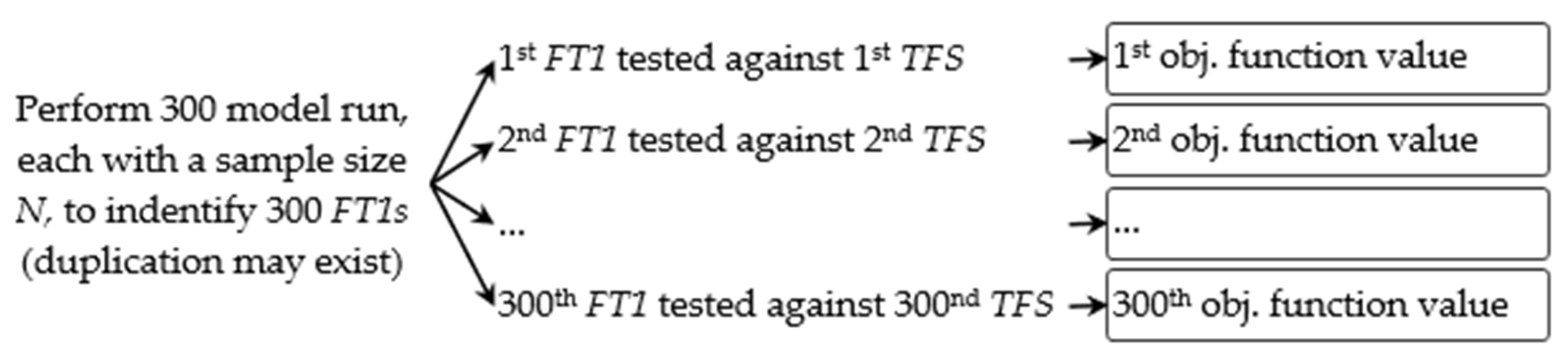
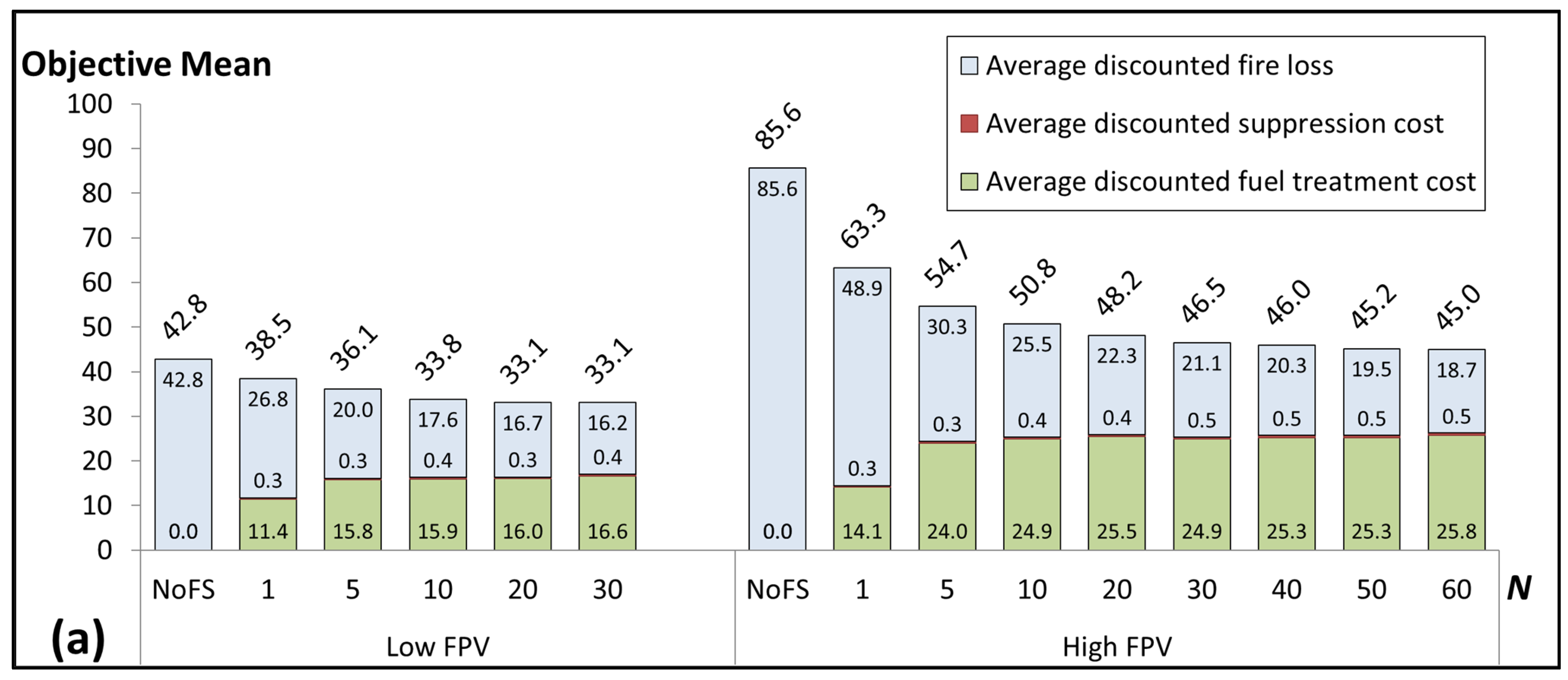
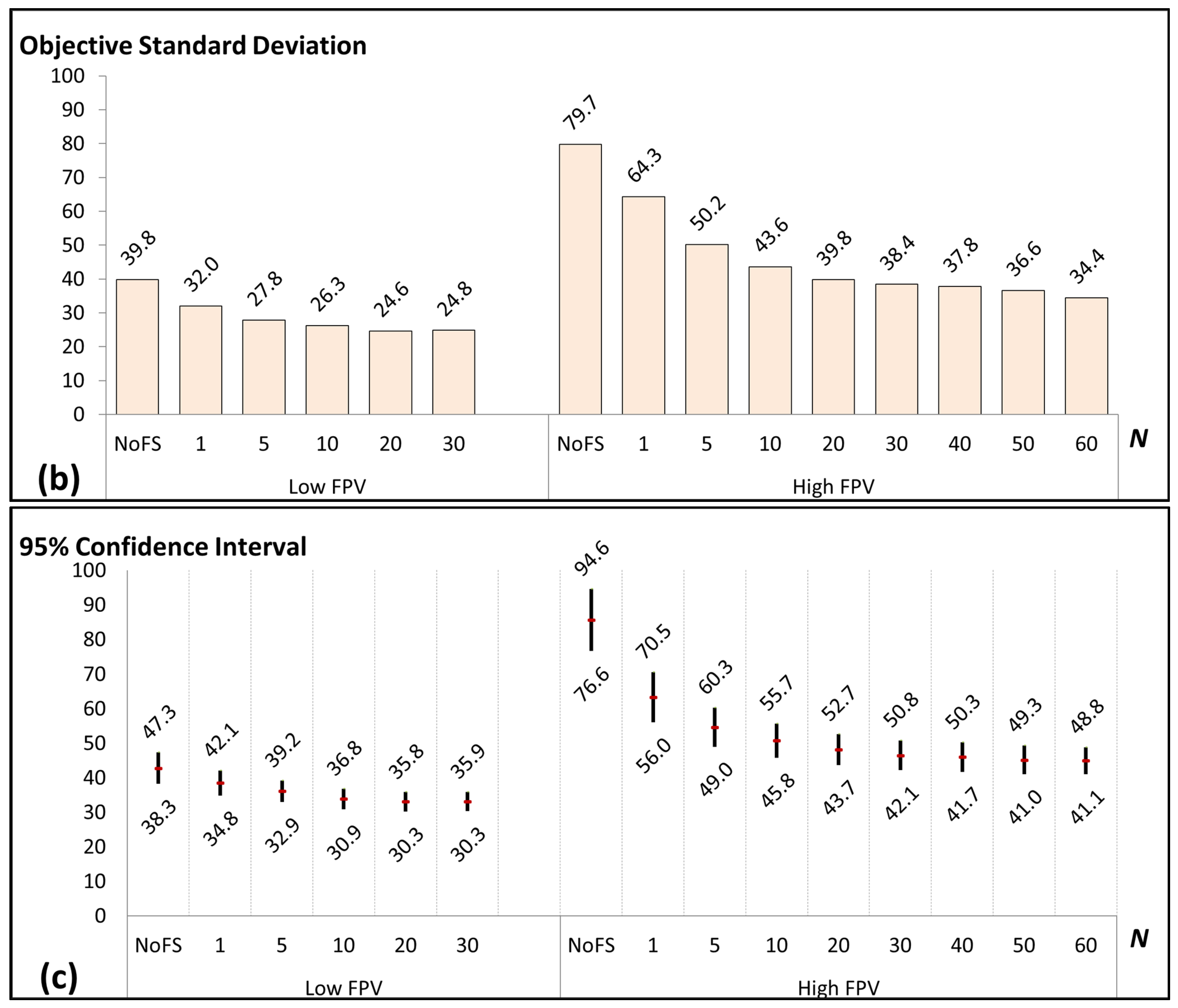
  • Test case 1—Examining the impact of sample size on the quality of the first period prescribed burning solutions (Figure 5). For every preselected sample size N, 300 stochastic model runs were conducted to identify a pool of 300 FT1s. An additional run was performed to test each FT1 solution in this pool against a random TFS in the fire testing set. An already tested TFS would not be used again to test another FT1 in this pool. When testing each FT1 solution against each TFS, the first period prescribed burning decision was hardcoded, but recourse decisions (both prescribed burning and fire suppression in later periods) were allowed to change to adapt to that TFS. The mean, standard deviation, and confidence interval of the objective function values from testing each pool of FT1s associated with a specific sample size N were calculated.
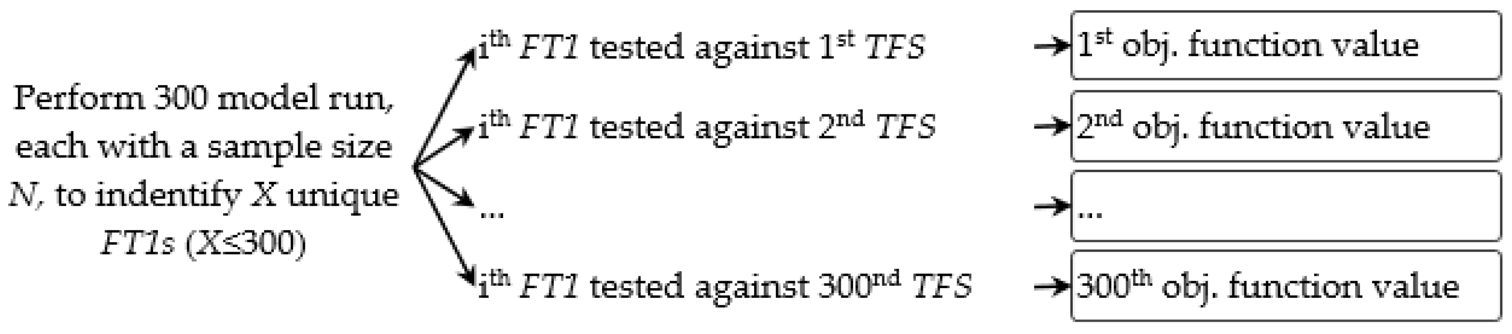
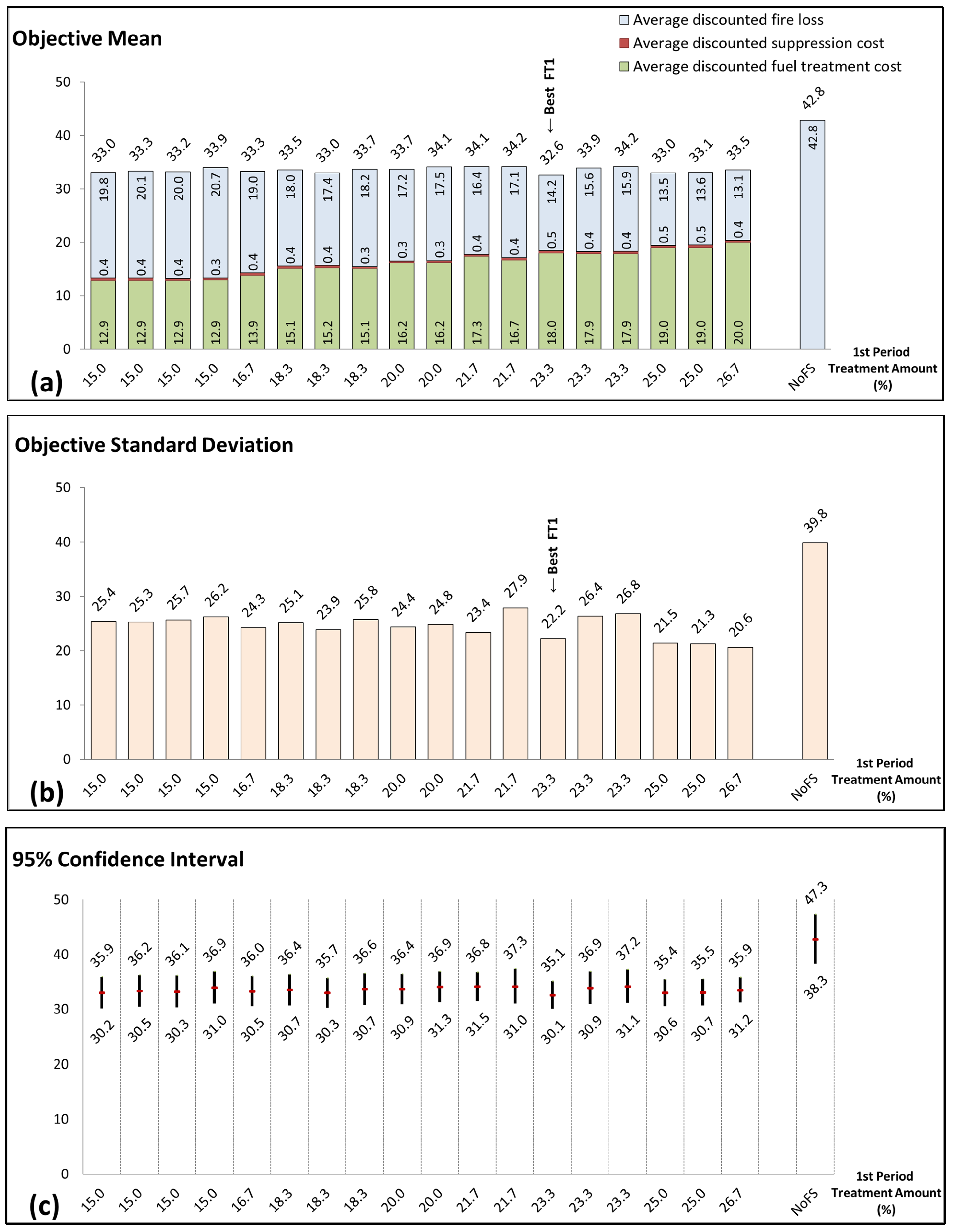
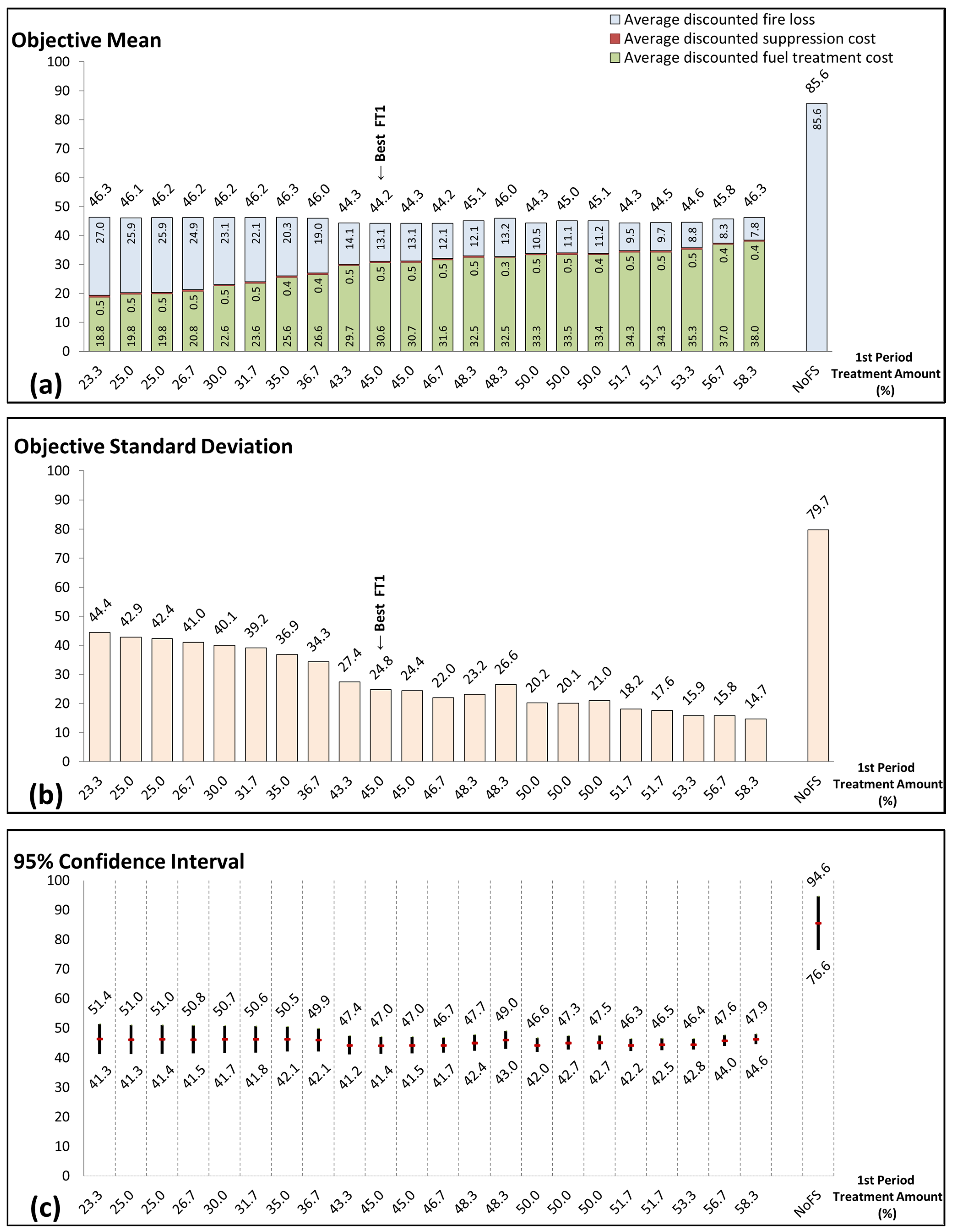
  • Test case 2—Examining the quality of period one prescribed burning decisions (Figure 6). For this test case, we ran the stochastic program 300 times with a preselected sample size N and evaluate all of the unique FT1s generated from these runs. Duplicated FT1s might exist, so the number of unique FT1s would be less than 300. The performance of each unique FT1 was also evaluated by using the fire testing set. The testing process would require 300 new model runs where sample size is set to one. In each run, the same unique FT1 solution was hardcoded and tested against a different TFS. The mean, standard deviation, and confidence interval of the objective function values from testing each unique FT1 was calculated to evaluate the quality of the FT1. Paired-t-tests were used to compare the quality of different unique FT1s.
Results from both test cases were reported for the two assumptions of the relative forest value to be protected (i.e., the low FVP, and the high FVP that is twice of the low FVP).

4. Results

4.1. Reference Test Case: No Fuel Treatment and Suppression

A reference test case (NoFS) was built by running the stochastic program to calculate fire loss from every TFS in the fire testing set when all fires were allowed to burn freely without interference from fuel treatment or suppression. For this test, 101 out of the 300 TFSs had no fire while the other 199 TFSs encountered one to five random fires in the three-decade planning horizon. The average size of a free-burning fire is ten cells (16% of the total landscape area). Without fuel treatment and suppression, the mean (and standard deviation) of the discounted fire loss was 42.8 (and 39.8) under the low FVP, and 85.6 (and 79.7) under the high FVP assumption.

4.2. Test case 1: Impact of Sample Size on the Quality of the First Period Prescribed Burning Solutions

One challenge in implementing the SAA method is to select an appropriate sample size that balances the model performance and computation time. Using a small sample size requires less computation time. In contrast, using larger sample sizes is more computationally expensive, but provides better outcomes in SAA. Table 2 illustrates the tradeoffs in our test.
Model solutions with a lower objective function mean were considered as producing better quality FT1s to deal with stochastic fire situations [118]. Results from the test case one (Figure 7) show that using a larger sample size would lead to a lower objective function mean (Figure 7a), a smaller standard deviation (Figure 7b), and a narrower confidence interval of the objective function mean (Figure 7c).
Increasing sample size can improve the overall quality and robustness of the FT1s generated by the stochastic program. However, this effect diminishes when sample size grows as indicated by less improvement for the means and standard deviations. Under the assumption of low FPV (and high FPV), we saw 12.0% (and 19.8%) reductions of the objective function mean, and 18.1% (and 32.2%) reduction of standard deviation when sample size increases from 1 to 10. Results from models using larger sample size were more robust, indicated by smaller differences of the objective function means. For example, the maximum difference of the means was less than 2.5% among models using sample size ≥ 10 under low FPV assumption and among models using sample size ≥ 40 under high FPV assumption.

4.3. Test Case 2: Quality of the First Period Prescribed Burning Decisions

Fuel treatment decisions at the first stage (or first period) need to be carried out immediately before the reveal of future fire conditions, and it may have impact on future fire behaviors and management recourse decisions at later stages. A good FT1 should consider the future fire situations and recourse activities. Using different sets of random sample fires or changing sample size N may suggest different FT1s. Selecting a good FT1 from those different solutions is often challenging.
Repetitively running the stochastic program using larger sample sizes can increase the chance of finding a good quality FT1. However, increasing sample size also makes the stochastic program more complex and consequently more difficult to solve. As indicated by the test case 1, solution quality will increase in a diminishing manor when sample size grows. This makes it possible to obtain a good set of FT1s using moderate sample sizes.
Under the assumption of low FPV, we selected a sample size of 30 DFSs to run the stochastic program 300 times and found 90 unique FT1s; each of them selects a different set of stands for prescribed burning in the first period. Under the high FPV assumption, the sample size of 60 DFSs was selected to run the stochastic program 300 times which identified 90 unique FT1s. The performance of each FT1 was then evaluated through paired-t-tests. We focused on studying those high-quality solutions (including “the best solution” with the lowest objective function mean found so far and the “alternative FT1s” that have less than 5% difference of the means compared to the best solution). Those high-quality FT1s were listed in Table 3 and illustrated in Figure 8 and Figure 9.
The paired t-test selection method suggested that the objective function value means from alternative FT1s and the best FT1 are not significantly different (Figure 8c and Figure 9c). However, increasing the total area of the first period prescribed burning would often decrease the average discounted loss from future fires (Figure 8a and Figure 9a), which also lowers the objective function standard deviations and creates narrower confidence intervals. This patten is more obvious when testing under the high FPV assumption (Figure 9b,c).
The best period-one prescribed burning decision under the low FPV (and high FPV) assumption was to treat stand 6 (and stands 1,6,9) which covers 23.3% (and 45%) of the total landscape area (Figure 10). In both best treatment solutions under the low and high FPV assumptions, treated stands separate the whole landscape into multiple patches. Results showed that the best FT1s decreased the objective mean significantly in comparison with NoFS, with 23.8% and 48.4% reduction rates respectively for the low and high FPV assumptions.
In addition to the best FT1s, there were 17 and 21 high-quality alternative FT1s respectively identified for the low and high FPV assumptions (Table 3). A good prescribed burning plan should treat between 15.0% and 26.7% of the total landscape areas during the first period when the FPV was low. If the FPV was doubled (the high FPV case), treated areas in the first period should cover 23.3% to 58.3% of the total landscape. Some treatment layouts of those selected alternatives were illustrated in Figure 11 and Figure 12.
Fire suppression decisions are modeled as a recourse decision in the SAA model to reflect the effectiveness of prescribed burning in lowing fire intensity and creating more suppression opportunities. Test results under both assumptions of the FPV suggested relatively low levels of fire suppression effort and cost. A potential reason is we assumed suppressions would only be allowed in cells with surface fires. Many suppression activities (and associated cost) in real-world may occur to control high intensity fires. Those costs were not included in our current program.

5. Conclusions and Discussion

Wildfire, along with the uncertainties associated with it, creates significant challenges in wildland fire management. Deterministic models often lack the capability to adequately capture the stochastic nature of wildfires, which may lead to biased management [60]. Optimizing wildfire decisions under a stochastic modeling framework has the advantage of providing more robust decisions by explicitly accounting for those uncertainties. We can choose to either draw random fire samples or construct representative fire scenarios to capture the effects of uncertainties in impacting management decisions. In this study, we used random fire samples to build a prototype SAA stochastic program that aims to minimize the expected sum of fire management cost and fire loss during a multi-period planning horizon. Several synthesized test cases were designed to examine the quality of prescribed fire decisions made in the first planning period that can support effective and efficient management of wildfires across the entire fire planning horizon.
The quality of prescribed burning decisions in the first period (or first stage) was our primary interest since this decision would need to be implemented immediately, whereas recourse decisions in later periods could be adjusted depending on the realizations of uncertainties. Using a multistage stochastic program would improve the robustness of the first period prescribed burning decision by accounting for uncertainties of future fire behavior and suppression activities.
From the perspective of optimization model development, one major contribution of this study is the integration of random wildfire occurrences and behaviors, prescribed burnings, and fire suppressions into one multistage stochastic program that can explicitly model the spatial and temporal interactions between these components. This level of integration has not been achieved by other optimization models developed so far according to our knowledge.
Another major contribution of this study is the design and use of a Monte Carlo-based heuristic to select high-quality period-one prescribed burning solutions by comparing and evaluating the pool of many candidate solutions acquired from multiple stochastic model runs. As expected, our results showed that using larger sample sizes in each SAA would improve solution robustness and efficiency, as indicated by lower values of both objective function means and standard deviations across a large number of replicated runs. The benefit of increasing sample size diminished as sample size increased, which justifies the use of a moderate sample size to obtain a reasonably good set of solutions. In our test cases, using sample size of 10 (or 30) to run models under the assumptions of low (or high) FPV could provide good quality period-one prescribed burning solutions.
Test cases in this study were built on a 12-stand forested landscape with synthesized fuel conditions and randomly simulated sample fires. Running this stochastic program on a larger landscape with more planning periods almost certainly requires using large sample sizes to obtain good quality solutions. Models built on a larger landscape are also difficult to solve. For example, we tested a 20-by-20 cell landscape including 70 stands using the same assumptions as in the current test cases; our computer could solve SAA models with the sample size up to 15 DFSs. Solving larger problems might be possible by using computer with more memory, developing more efficient modeling formulations, implementing proper heuristics, or employing other solution approaches such as decomposition methods. These hold potential for future research.
The stochastic program in this study focuses on addressing the prescribed-fire based fuel treatment decisions. This program, however, could be readily adapted without significantly altering its structure to consider other fuel treatment types. For example, the current program’s parameters could be easily modified to model treatment types that have different effects on fire spread rate ( R O S ( w , i , n ) , c c , R O S ( w , i , n ) , c c ) and intensity ( E ( w , i , n ) , c c , E ( w , i , n ) , c c ) and effectiveness durations ( W ). Some fuel treatment types, such as mechanical treatment, may increase the canopy base height (CBH) in a forest; the effect of treatment on increasing CBH can be modeled by setting up a higher threshold of fire line intensity to transit surface fires into crown fires. Incorporating various fuel treatment types into a single model is an interesting task in future research.
In this study, fire suppression was modeled as a simplified recourse decisions to select fire control locations for each future random fire. Our main purpose of modeling suppression was to reflect the fuel treatment effects in creating additional suppression opportunities instead of optimizing fire suppression decisions. Additional details of fire suppression activities such as crew movement, crew safety, line production, and line quality could be also included in a stochastic model as described by Belval et al. [119]. However, including that level of suppression details would result in a much complex model and requires further tests.
As an important component of forest management, the primary goal of fuel treatment is to lower future landscape fire risks. Due to the multi-objective nature of forest management, certain fuel treatment operations may contribute to or be conflicted with other forest management objectives as we described in the Introduction section. In addition, forest management operations such as biomass production may positively contribute to the task of fire risk mitigation [54]. Despite the general SAA program introduced in this study, it is often necessary to calibrate this program to account for multiple forest management objectives and to schedule multiple silviculture or fire risk mitigation methods to jointly achieve the long-term fire management goals.
As the final remark, this study presented a prototype SAA modeling structure and a Monte Carlo simulation-based solution selection mechanism to address a challenging prescribed fire location optimization problem. Preliminary results demonstrated the potential usage of this modeling structure to provide insight about the magnitude and spatial allocation of prescribed burning decisions to effectively fragment continuous forest fuels and create suppression opportunities.

Author Contributions

Conceptualization, D.N. and Y.W.; methodology, D.N. and Y.W.; software, D.N.; validation, D.N. and Y.W.; formal analysis, D.N.; investigation, D.N.; resources, D.N. and Y.W.; data curation, D.N. and Y.W.; writing—original draft preparation, D.N.; writing—review and editing, D.N. and Y.W.; visualization, D.N.; supervision, Y.W.; project administration, D.N. and Y.W. All authors have read and agreed to the published version of the manuscript.

Funding

This research received no external funding.

Data Availability Statement

The data presented in this study are available on request from the corresponding author.

Acknowledgments

Ministry of Education and Training of Vietnam and the Department of Forest and Rangeland Stewardship at Colorado State University for supporting the corresponding author during the PhD program.

Conflicts of Interest

The authors declare no conflict of interest.

Appendix A

A.1. Notations Used in the Stochastic Program Formulation

Notations including abbreviations, indices, parameters, sets, and variables used in the stochastic program formulation are introduced in Table A1. Some abbreviations are used frequently throughout this paper.
Table A1. Notations of the stochastic program formulation.
AbbreviationsDefinition
BEsThe beneficial effects of prescribed burning or wildfire. For example, areas recently treated by prescribed fire or burned by wildfire can decrease future fire intensity. These effects might last for certain period.
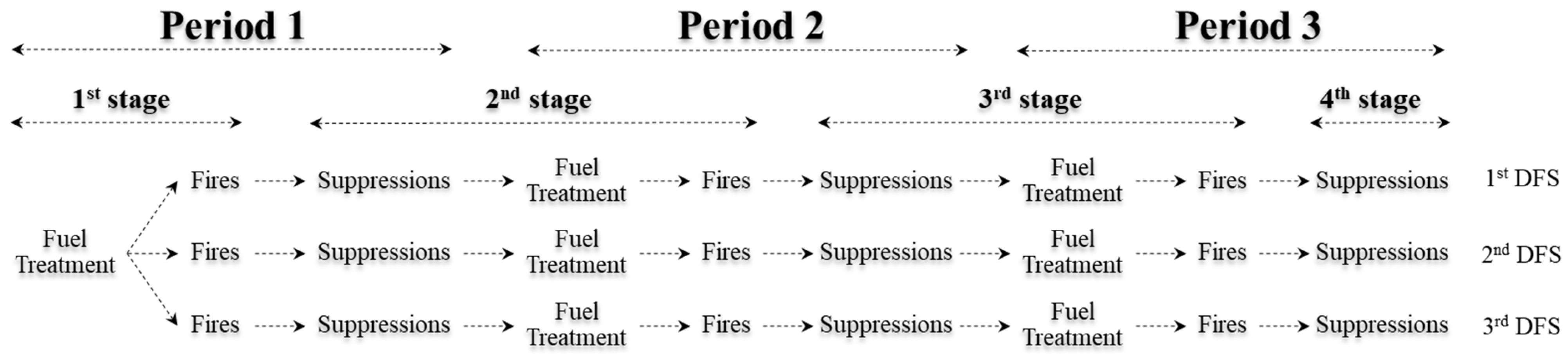
DFSA sequence of prescribed burning decisions, random fire events, and fire suppression decisions across all planning periods as illustrated in Figure 1.
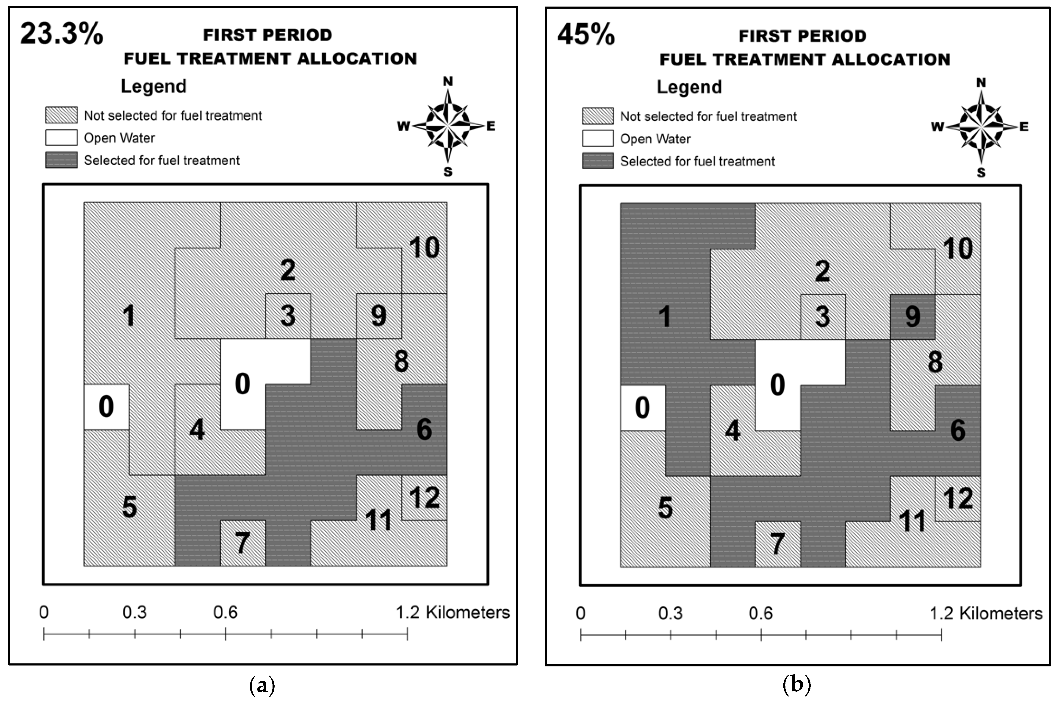
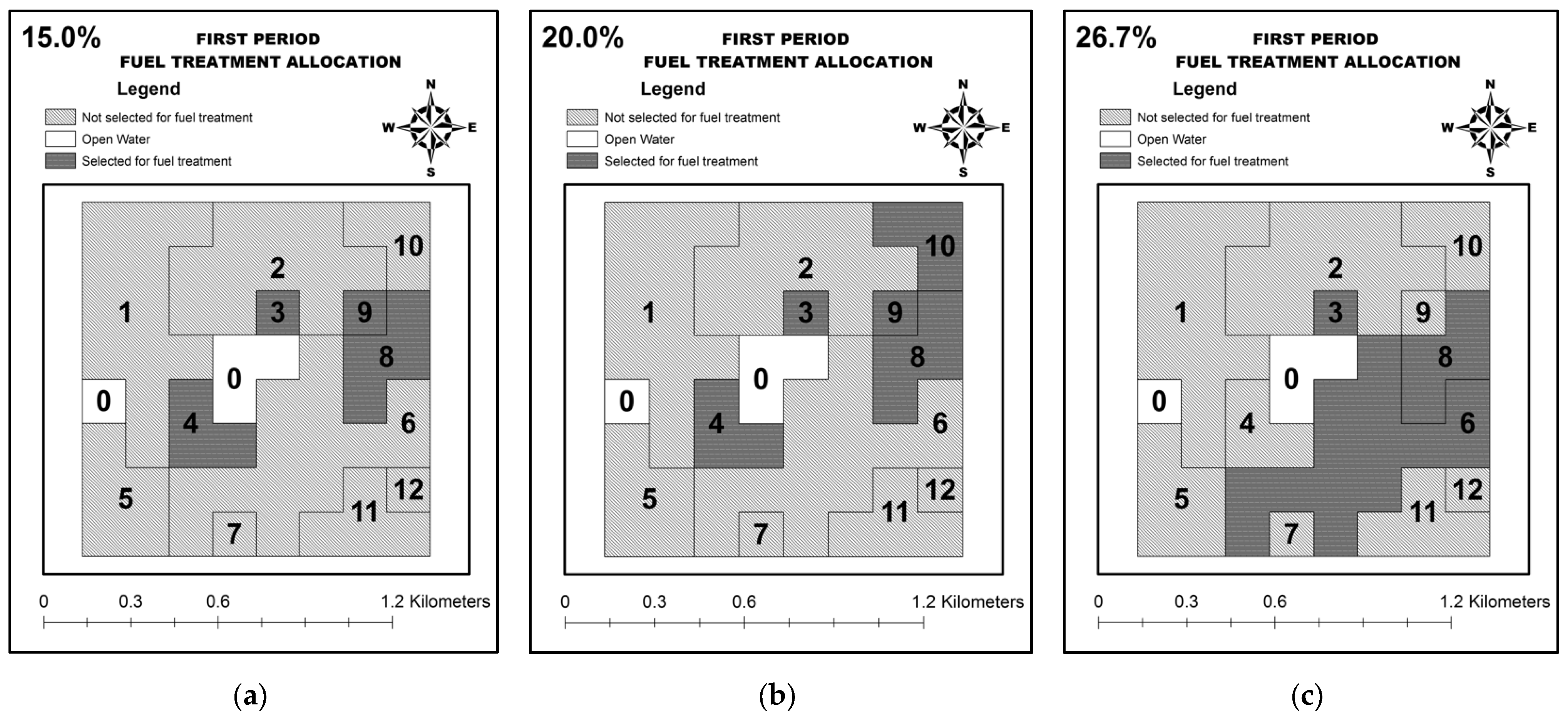
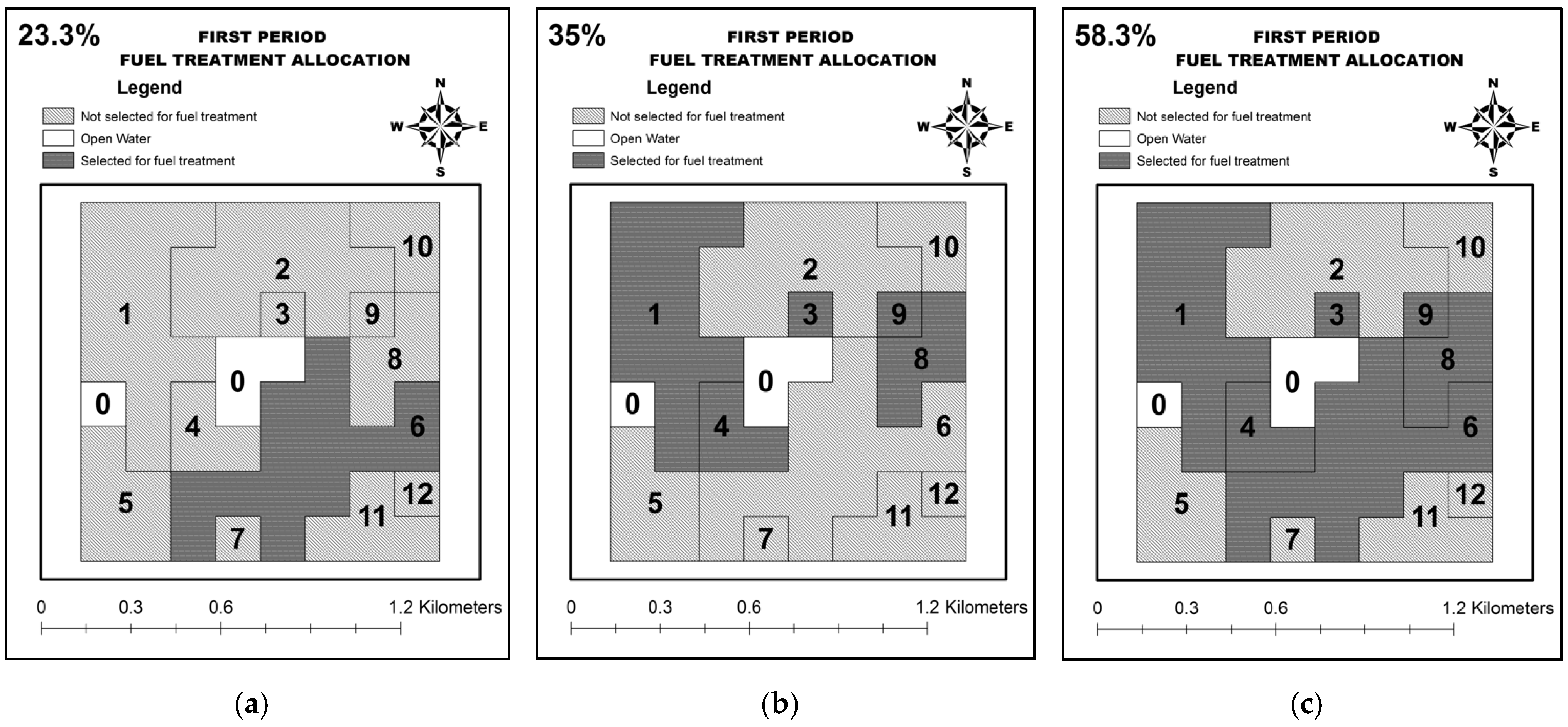
FT1The first period prescribed burning solution that includes a set of stands selected for prescribed burning at the beginning of the first period.
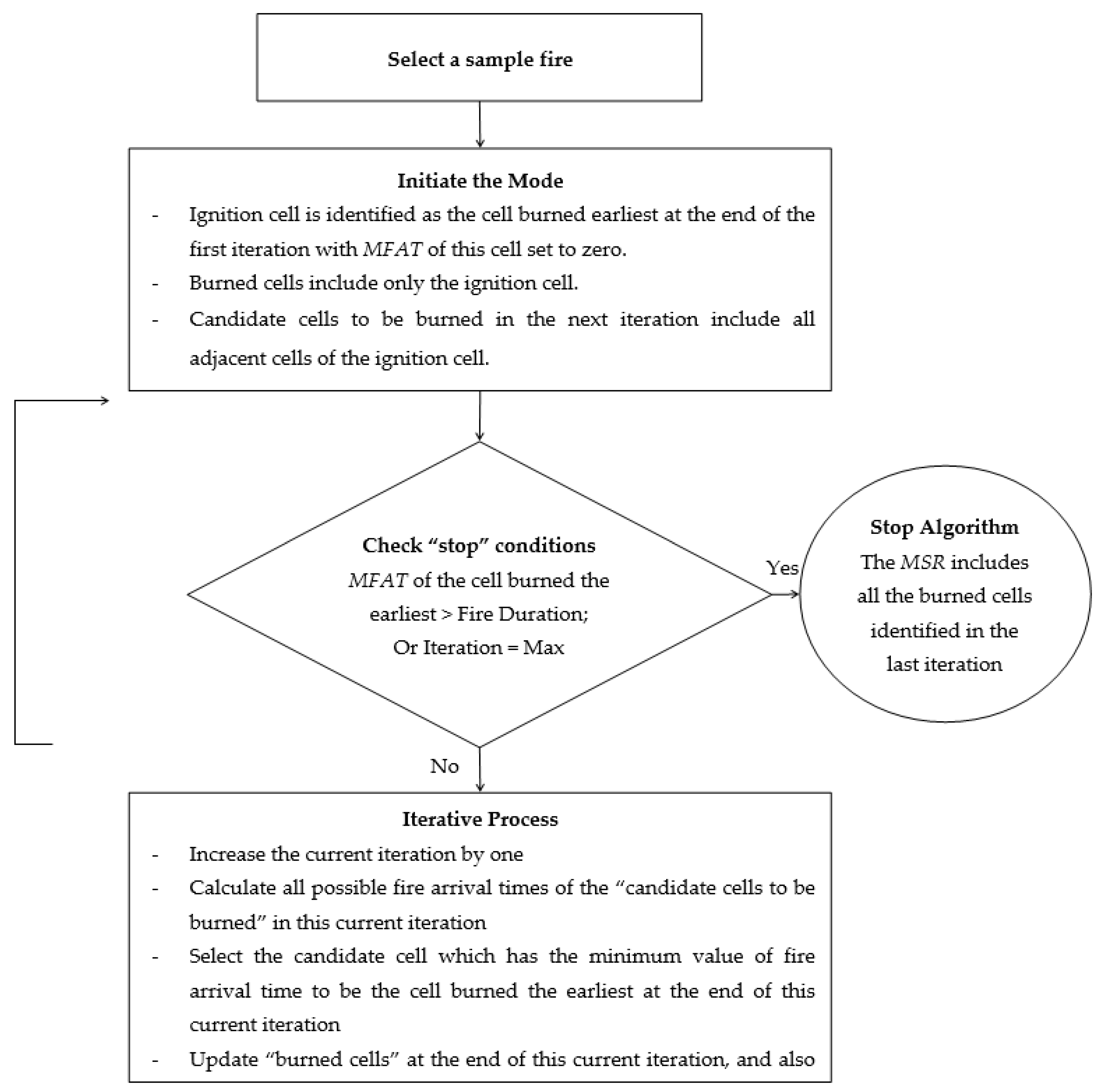
MFATThe “minimum fire arrival time” to each location (i.e., a cell) in a landscape. MFAT is calculated for every sample fire and every raster cell in the modeled landscape.
MSRThe “maximum spread range” of a sample fire calculated by a preprocessing algorithm (Appendix A.2)
IndicesDefinition
a Index of a stand.
a c Index of the stand that contains the raster cell c .
c , c Indices of raster cells.
i , i , i The occurrence order of sample fires in a planning period. For example, in a specific planning period a fire indexed by i = 1 would occur before the fire indexed by   i = 2 .
j Index of age-class of the forest in a raster cell.
n ,   n Indices of DFS samples.
w Index of a planning period.
( w , i , n ) An ordered set denotes the three attributes of a sample fire: w is the planning period when this fire occurs; i is the occurrence order of this fire in period w ; and n is the DFS in which this fire belongs.
ParametersDefinition
β c , c Half of the distance for a fire to spread from the center of cell c to the center of its adjacent cell c .
φ A small positive number.
C a The total number of cells within stand a .
C c The total number of adjacent cells of the cell c .
E c r i t i c a l ( w , i , n ) , c , j The critical threshold of fire line intensity in cell c when this cell is in age-class j at occurrence time of fire ( w , i , n ) . The fire ( w , i , n ) becomes crown fire in cell c when it burns cell c with the estimated fire line intensity meeting or exceeding this threshold.
E ( w , i , n ) , c c The fire line intensity in cell c if fire ( w , i , n ) spreads from c into c at spread rate R O S ( w , i , n ) , c c
G ( w , i , n ) , c A binary parameter: 1 if fire ( w , i , n ) ignites in cell c ; 0 if not.
H ( w , i , n ) The active spread duration of fire ( w , i , n ) determined exogenously through a random draw.
L ( w , i , n ) The time of occurrence (i.e., year) of sample fire ( w , i , n ) .
L w The time (i.e., year) at the beginning of period w when prescribed burning is scheduled (e.g., in case using 10-year planning period: L w = 1 = 0 , L w = 2 = 10 , and L w = 3 = 20 ).
M A large positive number (Big M).
N The total number of DFS samples. In this paper, the term “sample size” is used to represent N .
P F T The cost of prescribed burning in a cell if that cell has been neither treated by prescribed fire within W planning periods nor burned within W planning periods.
P F T The cost of prescribed burning in a cell if that cell has been treated by prescribed fire within W planning periods or burned within W planning periods. We assume P F T < P F T .
P S U P c The cost for fire control effort in cell c during suppression of a fire.
R An adopted annual discount rate.
R O S ( w , i , n ) , c c   R O S ( w , i , n ) , c c R O S ( w , i , n ) , c c is the estimated spread rate of fire ( w , i , n ) in cell c when this fire spreads into c from its adjacent cell c . If cell c is still influenced by the BEs of previous prescribed burning or wildfires, the spread rate in this cell would be R O S ( w , i , n ) , c c
R O S ( w , i , n ) , c c   R O S ( w , i , n ) , c c R O S ( w , i , n ) , c c is the estimated spread rate of fire ( w , i , n ) in cell c when this fire spreads from c to its adjacent cell c . If cell c is still influenced by the BEs of previous prescribed burning or wildfires, the spread rate in this cell would be R O S ( w , i , n ) , c c
V c , j The value to be protected in cell c when the forest in this cell is in age-class   j .
V ( w , i , n ) , c , j Fire loss in cell c if the forest in this cell is in age-class j at occurrence time of fire ( w , i , n ) and this fire burns as surface fire in c.
W The total number of planning periods in the entire planning horizon.
W The number of continuous planning periods in which the BEs from prescribed burning would last.
W The number of continuous planning periods in which the BEs from wildfire would last.
SetsDefinition
A ^ The set of all stands in a landscape.
C ^ The set of all cells in a landscape.
C ^ A c t i v e ( w , i , n ) The set of flammable cells inside the MSR of fire ( w , i , n ) .
C ^ a The set of all cells in stand a .
C ^ c The set of adjacent cells to cell c (sharing an edge or a vertex with c , excluding non-flammable cells).
C ^ I g n i t i o n ( w , i , n ) The ignition cell of fire ( w , i , n ) exogenously selected by random draws.
C ^ I n A c t i v e ( w , i , n ) The set of cells that are either non-flammable or outside the MSR of fire ( w , i , n ) .
VariablesDefinition
b ( w , i , n ) , c , c A binary variable: 1 if fire ( w , i , n ) successfully spreads from cell c into its adjacent cell c , and the spread path from c to c must belong to the fastest spread route of this fire to c ; 0 if not.
d ( w , i , n ) , c A binary variable: 1 if fire ( w , i , n ) burns cell c ; 0 if not.
e ( w , i , n ) , c A continuous variable to calculate the fire line intensity in cell c if it is burned by fire ( w , i , n ) when this fire spreads following its fastest spread route into cell c .
f F L n A continuous variable to calculate the total discounted fire loss for the nth DFS.
f F T n A continuous variable to calculate the total discounted cost of prescribed burning for the nth DFS.
f F T w , n A continuous variable to calculate the total discounted cost of prescribed burning scheduled in period w for the nth DFS.
f S U P n A continuous variable to calculate the total discounted cost of building fire-control-line for the nth DFS.
o ( w , i , n ) , c A binary variable: 1 if either fire ( w , i , n ) does not burn cell c or it burns as surface fire in cell c ; 0 if fire ( w , i , n ) burns as crown fire in cell c .
p ( w , i , n ) , c A binary variable: 1 if at occurrence time of fire ( w , i , n ) , cell c has been treated by prescribed fire within W planning periods or burned within W planning periods; 0 if not.
q ( w , i , n ) , c , j A binary variable: 1 if the forest in cell c is in age-class j at occurrence time of fire ( w , i , n ) ; 0 if not.
r ( w , i , n ) , c A binary variable: 1 if fire control effort is put into cell c to protect that cell from being burned by fire   ( w , i , n ) ; 0 if not.
s w , a , n For the nth DFS, this integer variable calculates the total number of cells in stand a in period w that have not been treated by prescribed fire within W planning periods and burned within W planning periods.
t ( w , i , n ) , c A continuous variable to track the MFAT of cell c , which is calculated based on the fastest route for fire ( w , i , n ) to spread into the center of c .
v C r o w n ( w , i , n ) , c , j A binary variable: 1 if fire ( w , i , n ) burns as crown fire in cell c and this cell is in age-class j at occurrence time of fire ( w , i , n ) ; 0 if not.
v S u r f a c e ( w , i , n ) , c , j A binary variable: 1 if fire ( w , i , n ) burns as surface fire in cell c and this cell is in age-class j at occurrence time of fire ( w , i , n ) ; 0 if not.
x w , a , n A binary variable: 1 if prescribed burning is implemented at the beginning of period w in stand a in the nth DFS; 0 if not.
y ( w , i , n ) , c A binary variable: 1 if either fire control effort has been put in cell c or the MFAT for fire ( w , i , n ) arriving the center of cell c is greater than that fire’s active spread-duration; 0 if not.
z w , c , n A binary variable: 1 if at the beginning of period w in the nth DFS, cell c is identified as not being treated by prescribed fire within W planning periods or burned within W planning periods; 0 if not.

A.2. A preprocessing Algorithm to Calculate the Maximum Spread Range (MSR) of a Sample Fire

This algorithm is used to calculate the MSR for each sample fire within an assumed duration, under a modeled wind condition, and without interference from fuel treatments, suppressions, and previous fires. A fire cannot spread beyond its MSR in future modeling when the effects of the previous fires, fuel treatments, or suppressions are to reduce fire spread rate and contain fires. Therefore, in the stochastic program suppression and fire spread will not be modeled outside of the MSRs. This preprocessing algorithm can help reduce computer memory consumption and also speed up solution time of the stochastic program.
This algorithm uses an iterative process to model fire spread. Fire can spread between adjacent cells sharing an edge or a vertex. At the end of each iteration, only one cell with the earliest fire arrival time would be identified as the cell that the fire will spread to in this iteration. The MSR of the simulated sample fire includes all of the burned cells identified in the last iteration. The algorithm is described by a flowchart (Figure A1) and an illustrative example (Figure A2).
Figure A1. A flowchart of the preprocessing algorithm to calculate the MSR of a sample fire.
Forests 13 00930 g0a1
Figure A2. An example to illustrate the preprocessing algorithm. In this example, a rectangular landscape including 42 cells is used to examine fire-spread-pattern for the first two iterations, assuming “stop” criteria are not met yet. The number in each cell represents the cell’s ID. There are two non-flammable cells (i.e., open water represented by the two blue cells 17 and 27) and 40 flammable cells (i.e., forest). The arrows represent all possible fire spread paths to the “candidate cells to be burned” (green) in the next iteration. In this ex-ample, cell 15 is assumed to be the fire’s ignition cell, which is the cell burned earliest at the end of iteration one. At iteration two, fire can spread from cell 15 to its eight “candidate cells to be burned” (8, 9, 10, 14, 16, 20, 21, and 22). The fire is assumed to spread from cell 15 to cell 22 faster than spreading to the other seven cells. Under this assumption, cell 22 would be identified as the cell burned earliest at the end of the second iteration.
Forests 13 00930 g0a2

A.3. Book-Keeping Variables and Constraints Used in the Stochastic Program Formulation

This section presents variables and constraints that were also used in the stochastic program formulation but were not mentioned in the main text (i.e., Section 2). Since these variables and constraints are either book-keeping values or intermediate calculations, moving them to Appendix can help decrease the density of equations in the main text for better communication of the key aspects of our model formulation.
Variables:
  • k ( w , i , n ) , c , w w 
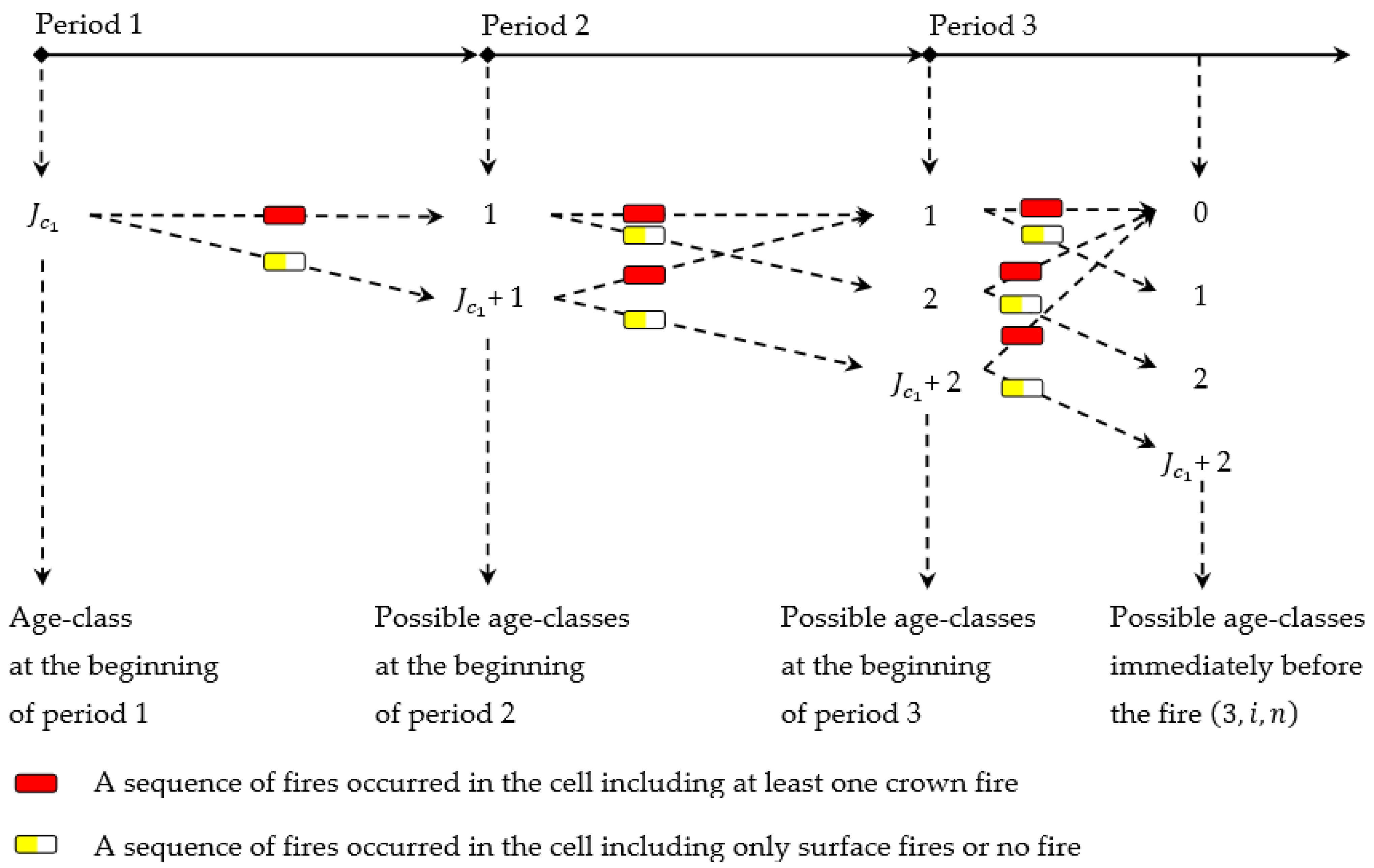
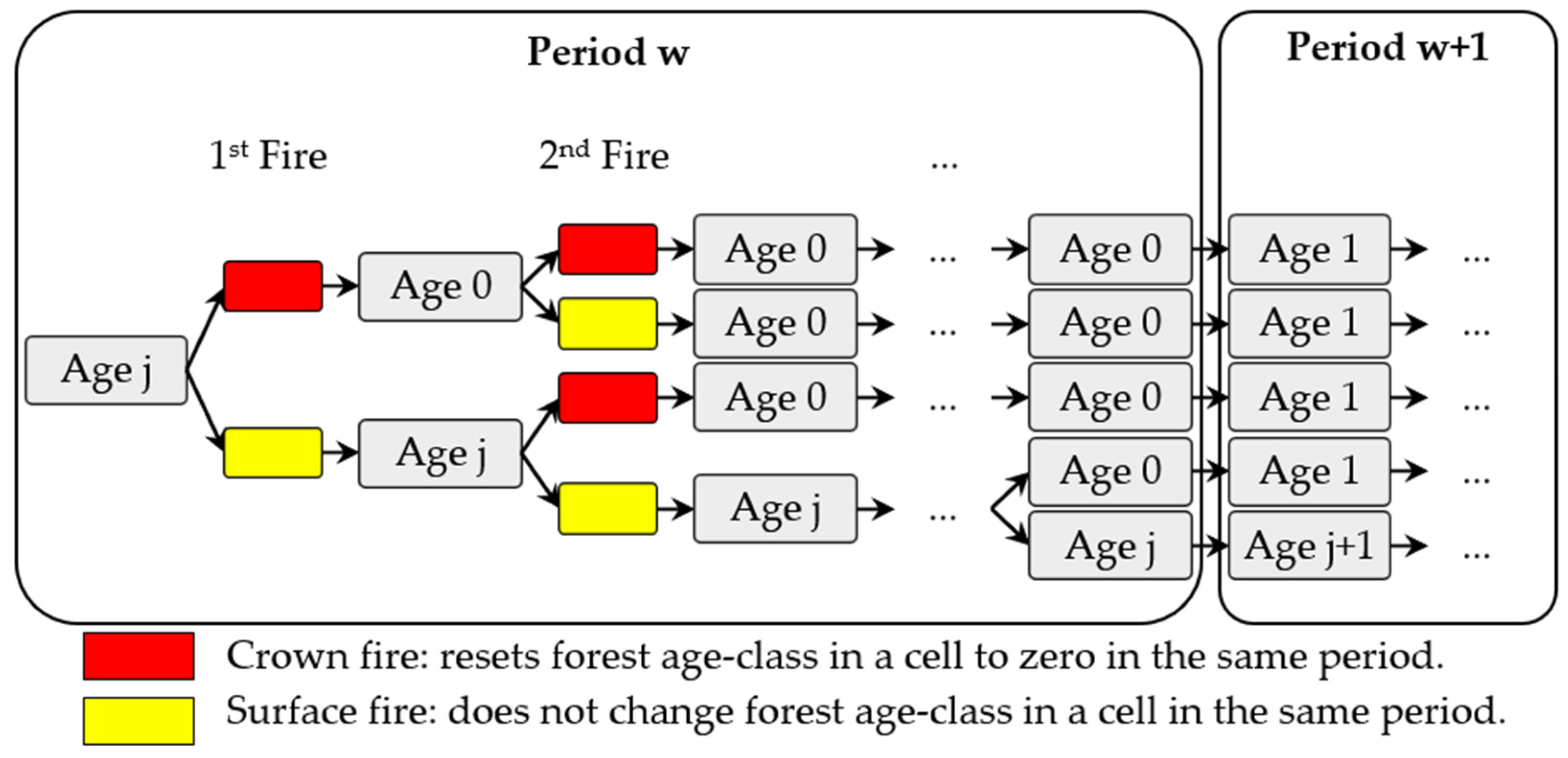
: A binary variable receiving a value of one if at least one crown fire has occurred in cell c in period w before occurrence time of fire ( w , i , n ) ; otherwise, k ( w , i , n ) , c , w w = 0 .
  • u ( w , i , n ) , c , j : A binary variable receiving a value of one if cell c in age-class j is burned by fire ( w , i , n ) . If either cell c is not in age-class j or fire ( w , i , n ) does not burn this cell then u ( w , i , n ) , c , j = 0 .
Constraints:
At the beginning of each planning period, cells that have been “treated within W planning periods or burned within W periods” are tracked by Equations (A1)–(A3), and the total number of such cells ( s w , a , n > 0 ) is identified for each stand (Equation (A4)) only when prescribed burning is implemented in the stand ( x w , a , n = 1 ) (Equation (A5)); otherwise, s w , a , n is set to zero.
z w , c , n x w , a c , n c C ^ , n , w ,   w W ^ w
z w , c , n d ( w , i , n ) , c c C ^ ,   i ,   n , w ,   w W ^ w
z w , c , n M × ( x w , a c , n + w W ^ w i d ( w , i , n ) , c ) c C ^ , n , w ,   w W ^ w
s w , a , n c C ^ a z w , c , n a A ^ , n , w
s w , a , n M × x w , a , n a A ^ , n , w
In this model, forest age-class of a cell is identified at the time immediately before the occurrence of each fire (by q ( w , i , n ) , c , j variable). Each time when a fire ( w , i , n ) occurs, past fire situations in each cell will be tracked (Equations (A6) and (A7)) and used to identify the forest age class of that cell at the occurrence time of fire ( w , i , n ) (Equations (A8)–(A11)).
k ( w , i , n ) , c , w 1 o ( w , i , n ) , c   c C ^ A c t i v e ( w , i , n ) , i , i < i   i f   w = w , n , w , w w
k ( w , i , n ) , c , w i :   i < i   i f   w = w ( 1 o ( w , i , n ) , c )   c C ^ A c t i v e ( w , i , n ) , i , n , w , w w
q ( w , i , n ) , c , j = 0   c C ^ A c t i v e ( w , i , n ) , i , j J ^ ( w , i , n ) , c , n , w
q ( w , i , n ) , c , j = 0 = k ( w , i , n ) , c , w = w   c C ^ A c t i v e ( w , i , n ) , i , n , w
q ( w , i , n ) , c , j k ( w , i , n ) , c , w = w j w W ^ j , w k ( w , i , n ) , c , w   c C ^ A c t i v e ( w , i , n ) , i , j J ^ ( w , i , n ) , c \ { 0 , J c 1 + w 1 } , n , w
j J ^ ( w , i , n ) , c q ( w , i , n ) , c , j = 1   c C ^ A c t i v e ( w , i , n ) , i , n , w
The logic of Equations (A8)–(A11) can be described by the following example (see Figure A3 for illustration of the logic). In this example, we assume the age-class of forest in the cell c is J c 1 at the beginning of the first period. We use an example set of three fires in three continuous planning periods denoted by fire ( 1 , i , n ) , fire ( 2 , i , n ) , and fire ( 3 , i , n ) . Each of these three fires can occur before or after the occurrences of other fires in the same period.
  • For fire ( 1 , i , n ) in the 1st period: Age-class of cell c at the time immediately before the occurrence of fire ( 1 , i , n ) can be either 0 or J c 1 ( J ^ ( 1 , i , n ) , c = { 0 , J c 1 } )
  • For fire ( 2 , i , n ) in the 2nd period: Age-class of cell c at the time immediately before the occurrence of fire ( 2 , i , n ) can only be 0, 1, or J c 1 + 1 ( J ^ ( 2 , i , n ) , c = { 0 , 1 , J c 1 + 1 } )
  • For fire ( 3 , i , n ) in the 3rd period: Age-class of cell c at the time immediately before the occurrence of fire ( 3 , i , n ) can only be 0, 1, 2, or J c 1 + 2 ( J ^ ( 3 , i , n ) , c = { 0 , 1 , 2 , J c 1 + 2 }
Equations (A12) and (A13) works together to guarantee that if a fire burns a cell ( c ) then it only burns that cell at its exact (or current) age-class (the age-class immediately before the occurrence of this fire). A fire occurrence can lead to only one of the three situations of a cell ( c ) at its current age-class: not being burned by the fire ( d ( w , i , n ) , c = 0 ); being burned by the fire as surface fire in this cell ( v S u r f a c e ( w , i , n ) , c , j = 1 ); or being burned by the fire as crown fire in this cell ( v C r o w n ( w , i , n ) , c , j = 1 ) (Equation (A14)). Equations (A15) and (A16) are used to track one of those situations, when a fire burns as crown fire in a cell ( c ) at its current age-class ( j ) ( v C r o w n ( w , i , n ) , c , j receives the value of one only for the case when o ( w , i , n ) , c = 0 and q ( w , i , n ) , c , j = 1 ). The three equations (A14)–(A16) work together to identify the exact fire situation in each cell at its current age-class when a fire occurs. This can help calculate the exact fire loss for each fire.
u ( w , i , n ) , c , j d ( w , i , n ) , c + q ( w , i , n ) , c , j 1   c C ^ A c t i v e ( w , i , n ) , i , j , n , w
u ( w , i , n ) , c , j q ( w , i , n ) , c , j + d ( w , i , n ) , c 2   c C ^ A c t i v e ( w , i , n ) , i , j , n , w
v S u r f a c e ( w , i , n ) , c , j + v C r o w n ( w , i , n ) , c , j = u ( w , i , n ) , c , j   c C ^ A c t i v e ( w , i , n ) , i , j , n , w
v C r o w n ( w , i , n ) , c , j q ( w , i , n ) , c , j o ( w , i , n ) , c   c C ^ A c t i v e ( w , i , n ) , i , j , n , w
v C r o w n ( w , i , n ) , c , j 1 + q ( w , i , n ) , c , j o ( w , i , n ) , c 2   c C ^ A c t i v e ( w , i , n ) , i , j , n , w
Figure A3. Possible age-classes of the forest in a cell at different times during a three-period planning horizon, assuming the forest age-class in this cell is J c 1 at the beginning of the first period.
Forests 13 00930 g0a3

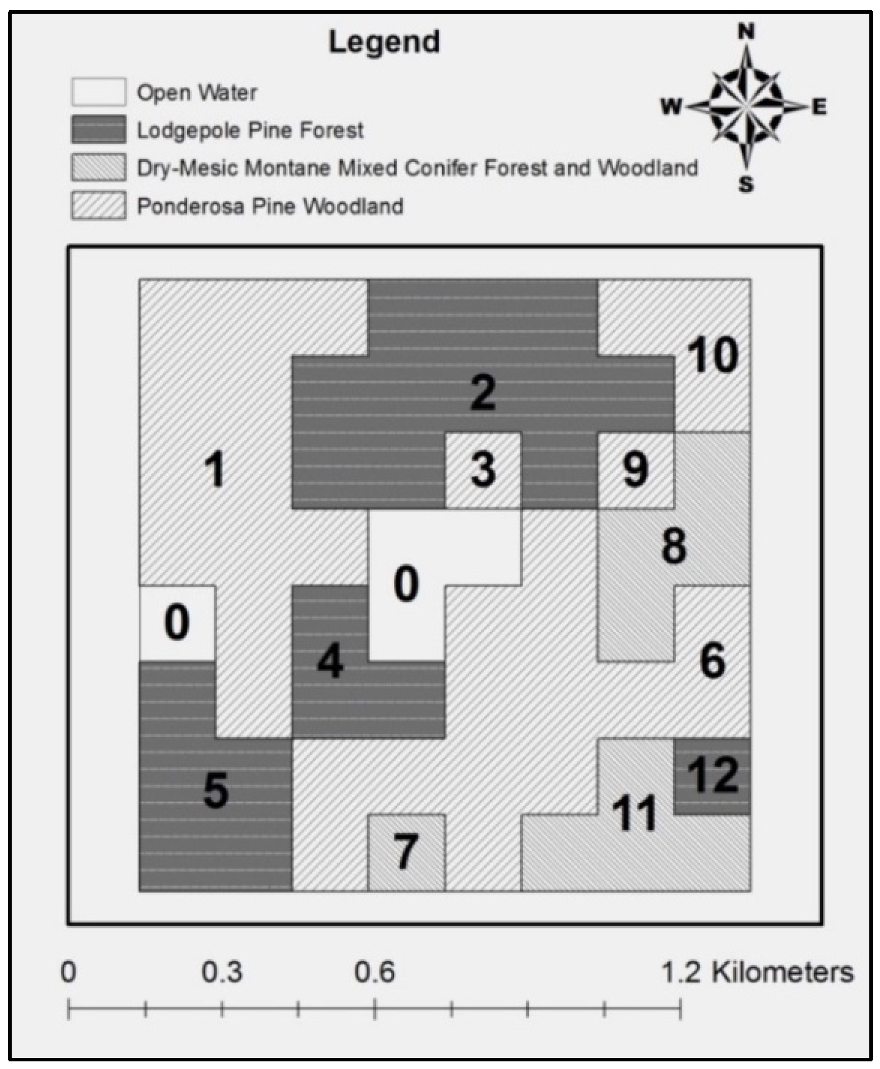
A.4. Information of the Synthesized Landscape

Topography (elevation, slope, aspect), forest cover, and fuel information of the landscape were based on the LANDFIRE data (www.landfire.gov, accessed on 30 August 2014) of a real forested area located in Larimer County, Colorado, USA. Wildfire ignition frequency in the landscape was created based on historical fire data in the same region. Wind conditions in the landscape were estimated based on the ten-year RAWS records between 2004 and 2013 collected from the Red Feather Lake station in Colorado. We assumed all forested cells in the landscape were at the age-class three and randomly assigned a canopy base height (CBH) of 3–4 m to each cell. Future forest age-class of a cell might change and would be associated with a CBH randomly generated within a specified range as listed in Table A2.
Table A2. Information used to build the test cases.
CharacteristicSpecification
Elevation2455–2587 m
Slope5–90%
Aspect0, 45, 90, 135, 180, 225, 270, 315, 360
Fuel model (Fuel type)Open Water (98)
Mixed Conifer Forest and Woodland (122)
Ponderosa Pine Woodland (165)
Lodge pole Pine Forest (183)
Canopy cover80–100%
Foliar moisture content (FMC)100%
Forest age-class;
Canopy base height (CBH)
Age   1   ( 1 10   years ) ;   1 2   m Age   2   ( 11 20   years ) ;   2 3   m Age   3   ( 21   years ) ;   3 4   m
Wildfire ignition frequency0.0078125 per cell per decade
Wind direction and speed16 combinations of wind direction and speed with cumulative percentage:
N, 4.5, 2%
NNE, 4 mph, 3.6%
NNW, 5 mph, 6.7%
NE, 4.9 mph, 11.4%
ENE, 4.6 mph, 14.7%
E, 5 mph, 19.4%
ESE, 5.3 mph, 27%
SE, 5.2 mph, 32%
SSE, 4.4 mph, 34.1%
S, 4.7 mph, 35.8%
SSW, 5.5 mph, 39%
SW, 5.2 mph, 52.2%
WSW, 6.6 mph, 65.3%
W, 7.8 mph, 80.8%
WNW, 8 mph, 93.4%
NW, 6.1 mph, 100%

A.5. FLAMMAP Outputs for Calculations of Parameters Used in the Test Cases

FLAMMAP version 1.5 was used to report the dimension of the assumed elliptical shape of fire spread in each cell. This information was used to calculate the spread rate, fire line intensity, and intensity threshold for transition from surface fire to crown fire in each cell; those parameters would be used in our two test cases. The spread rates in each cell following different spread directions ( R O S ( w , i , n ) , c c and R O S ( w , i , n ) , c c ) were calculated based on [120]. Fire line intensity in each direction ( E ( w , i , n ) , c c and E ( w , i , n ) , c c ) was calculated by Equations (A17) and (A18). The fire line intensity threshold for transition from surface fire to crown fire in each cell was calculated based on [121] as in Equation (A19).
E ( w , i , n ) , c c = E ( w , i , n ) , c × R O S ( w , i , n ) , c c R O S ( w , i , n ) , c
E c r i t i c a l ( w , i , n ) , c , j = ( 0.01 × C B H ( w , i , n ) , c , j × ( 460 + 25.9 × F M C ( w , i , n ) , c ) ) 1.5   c C ^ A c t i v e ( w , i , n ) , i , n , w
where: C B H ( w , i , n ) , c , j is the canopy base high of the forest in cell c at age-class j at the occurrence time of the fire ( w , i , n ) ; and F M C ( w , i , n ) , c is the foliar moisture content of cell c at the time the fire ( w , i , n ) ignites.

References

  1. King, K.J.; Bradstock, R.A.; Cary, G.J.; Chapman, J.; Marsden-Smedley, J.B. The Relative Importance of Fine-Scale Fuel Mosaics on Reducing Fire Risk in South-West Tasmania, Australia. Int. J. Wildland Fire 2008, 17, 421–430. [Google Scholar] [CrossRef]
  2. Kozlowski, T.T. Fire and Ecosystems; Elsevier: Amsterdam, The Netherlands, 2012; ISBN 0-323-14617-1. [Google Scholar]
  3. László, F.; Rajmund, K. Characteristics of Forest Fires and Their Impact on the Environment. AARMS Acad. Appl. Res. Mil. Public Manag. Sci. 2016, 15, 5–17. [Google Scholar]
  4. Alkire, C. The Federal Wildland Fire Budget, Let’s Prepare, Not Just React: Emphasis on Reduced Financial and Ecological Costs; Wilderness Society: Washington, DC, USA, 2004. [Google Scholar]
  5. Conard, S.G.; Hartzell, T.; Hilbruner, M.W.; Zimmerman, G.T. Changing Fuel Management Strategies—The Challenge of Meeting New Information and Analysis Needs. Int. J. Wildland Fire 2001, 10, 267–275. [Google Scholar] [CrossRef]
  6. Agee, J.K.; Skinner, C.N. Basic Principles of Forest Fuel Reduction Treatments. For. Ecol. Manag. 2005, 211, 83–96. [Google Scholar] [CrossRef]
  7. Cohen, J. The wildland-urban interface fire problem: A consequence of the fire exclusion paradigm. For. Hist. Today 2010, Fall, 20–26. [Google Scholar]
  8. Pyne, S.J.; Andrews, P.L.; Laven, R.D. Introduction to Wildland Fire; John Wiley and Sons: Hoboken, NJ, USA, 1996. [Google Scholar]
  9. Finney, M.A. Design of Regular Landscape Fuel Treatment Patterns for Modifying Fire Growth and Behavior. For. Sci. 2001, 47, 219–228. [Google Scholar]
  10. Collins, B.M.; Stephens, S.L.; Moghaddas, J.J.; Battles, J. Challenges and Approaches in Planning Fuel Treatments across Fire-Excluded Forested Landscapes. J. For. 2010, 108, 24–31. [Google Scholar]
  11. Fulé, P.Z.; McHugh, C.; Heinlein, T.A.; Covington, W.W. Potential Fire Behavior Is Reduced Following Forest Res-Toration Treatments. In Proceedings of the Ponderosa Pine Ecosystems Restoration and Conservation: Steps Toward, Flagstaff, AZ, USA, 25–27 April 2000. [Google Scholar]
  12. Martinson, E.J.; Omi, P.N.; Omi, P.N.; Joyce, L.A. Performance of Fuel Treatments Subjected to Wildfires; Citeseer: Princeton, NJ, USA, 2002. [Google Scholar]
  13. Fiedler, C.E.; Keegan, C.E., III.; Woodall, C.W.; Morgan, T.A. A Strategic Assessment of Crown Fire Hazard in Montana: Potential Effectiveness and Costs of Hazard Reduction Treatments; PNW-GTR-622; U.S. Department of Agriculture, Forest Service, Pacific Northwest Research Station: Portland, OR, USA, 2004. [Google Scholar]
  14. Skinner, C.N. Reintroducing Fire into the Blacks Mountain Research Natural Area: Effects on Fire Hazard. In Proceedings of the Conference on Symposium on Ponderosa Pine: Issues, Trends, And Management, Klamath Falls, OR, USA, 18–21 October 2004; Citeseer: Princeton, NJ, USA, 2005; pp. 245–257. [Google Scholar]
  15. Ritchie, M.W.; Skinner, C.N.; Hamilton, T.A. Probability of Tree Survival after Wildfire in an Interior Pine Forest of Northern California: Effects of Thinning and Prescribed Fire. For. Ecol. Manag. 2007, 247, 200–208. [Google Scholar] [CrossRef]
  16. Strom, B.A.; Fulé, P.Z. Pre-Wildfire Fuel Treatments Affect Long-Term Ponderosa Pine Forest Dynamics. Int. J. Wildland Fire 2007, 16, 128–138. [Google Scholar] [CrossRef]
  17. Schmidt, D.A.; Taylor, A.H.; Skinner, C.N. The Influence of Fuels Treatment and Landscape Arrangement on Simulated Fire Behavior, Southern Cascade Range, California. For. Ecol. Manag. 2008, 255, 3170–3184. [Google Scholar] [CrossRef]
  18. Stephens, S.L.; Moghaddas, J.J.; Edminster, C.; Fiedler, C.E.; Haase, S.; Harrington, M.; Keeley, J.E.; Knapp, E.E.; McIver, J.D.; Metlen, K. Fire Treatment Effects on Vegetation Structure, Fuels, and Potential Fire Severity in Western US Forests. Eco-Log. Appl. 2009, 19, 305–320. [Google Scholar] [CrossRef] [PubMed] [Green Version]
  19. Laverty, L.; Williams, J. Protecting People and Sustaining Resources in Fire-Adapted Ecosystems: A Cohesive Strategy; Citeseer: Princeton, NJ, USA, 2000. [Google Scholar]
  20. Radeloff, V.C.; Hammer, R.B.; Stewart, S.I.; Fried, J.S.; Holcomb, S.S.; McKeefry, J.F. The Wildland-Urban Interface in the United States. Ecol. Appl. 2005, 15, 799–805. [Google Scholar] [CrossRef] [Green Version]
  21. Ager, A.A.; McMahan, A.J.; Barrett, J.J.; McHugh, C.W. A Simulation Study of Thinning and Fuel Treatments on a Wildland–Urban Interface in Eastern Oregon, USA. Landsc. Urban Plan. 2007, 80, 292–300. [Google Scholar] [CrossRef]
  22. Contreras, M.A.; Parsons, R.A.; Chung, W. Modeling Tree-Level Fuel Connectivity to Evaluate the Effectiveness of Thinning Treatments for Reducing Crown Fire Potential. For. Ecol. Manag. 2012, 264, 134–149. [Google Scholar] [CrossRef]
  23. Gonzalez, J.R.; Barrio, G.; Duguy, B. Assessing Functional Landscape Connectivity for Disturbance Propagation on Regional Scales—A Cost-Surface Model Approach Applied to Surface Fire Spread. Ecol. Model. 2008, 211, 121–141. [Google Scholar] [CrossRef]
  24. Reinhardt, E.D.; Keane, R.E.; Calkin, D.E.; Cohen, J.D. Objectives and Considerations for Wildland Fuel Treatment in Forested Ecosystems of the Interior Western United States. For. Ecol. Manag. 2008, 256, 1997–2006. [Google Scholar] [CrossRef]
  25. Mell, W.E.; Manzello, S.L.; Maranghides, A.; Butry, D.; Rehm, R.G. The Wildland–Urban Interface Fire Problem–Current Approaches and Research Needs. Int. J. Wildland Fire 2010, 19, 238–251. [Google Scholar] [CrossRef]
  26. Bevers, M.; Omi, P.N.; Hof, J. Random Location of Fuel Treatments in Wildland Community Interfaces: A Percolation Approach. Can. J. For. Res. 2004, 34, 164–173. [Google Scholar] [CrossRef] [Green Version]
  27. Hirsch, K.G.; Podur, J.J.; Janser, R.F.; McAlpine, R.S.; Martell, D.L. Productivity of Ontario Initial-Attack Fire Crews: Results of an Expert-Judgement Elicitation Study. Can. J. For. Res. 2004, 34, 705–715. [Google Scholar] [CrossRef]
  28. Loehle, C. Applying Landscape Principles to Fire Hazard Reduction. For. Ecol. Manag. 2004, 198, 261–267. [Google Scholar] [CrossRef] [Green Version]
  29. Agee, J.K.; Bahro, B.; Finney, M.A.; Omi, P.N.; Sapsis, D.B.; Skinner, C.N.; Wagtendonk, J.W.; Weatherspoon, C.P. The Use of Shaded Fuelbreaks in Landscape Fire Management. For. Ecol. Manag. 2000, 127, 55–66. [Google Scholar] [CrossRef]
  30. Finney, M.A.; Cohen, J.D. Expectation and Evaluation of Fuel Management Objectives. In The USDA Forest Service Proceedings RMRS-P-29; USDA Forest Service: Washington, DC, USA, 2003; pp. 353–366. [Google Scholar]
  31. Moghaddas, J.J.; Craggs, L. A Fuel Treatment Reduces Fire Severity and Increases Suppression Efficiency in a Mixed Conifer Forest. Int. J. Wildland Fire 2008, 16, 673–678. [Google Scholar] [CrossRef]
  32. Carey, H.; Schumann, M. Modifying Wildfire Behavior—The Effectiveness of Fuel Treatments; National Community Forestry Center: Quebec, QC, Canada, 2003. [Google Scholar]
  33. Graham, R.T.; McCaffrey, S.; Jain, T.B. Science Basis for Changing Forest Structure to Modify Wildfire Behavior and Severity; RMRS-GTR-120; U.S. Department of Agriculture, Forest Service, Rocky Mountain Research Station: Fort Collins, CO, USA, 2004. [Google Scholar]
  34. Ager, A.A.; Finney, M.A.; Kerns, B.K.; Maffei, H. Modeling Wildfire Risk to Northern Spotted Owl (Strix Occidentalis Caurina) Habitat in Central Oregon, USA. For. Ecol. Manag. 2007, 246, 45–56. [Google Scholar] [CrossRef]
  35. Finney, M.A.; Seli, R.C.; McHugh, C.W.; Ager, A.A.; Bahro, B.; Agee, J.K. Simulation of Long-Term Landscape-Level Fuel Treatment Effects on Large Wildfires. Int. J. Wildland Fire 2008, 16, 712–727. [Google Scholar] [CrossRef] [Green Version]
  36. González, J.; Palahí, M.; Pukkala, T. Integrating Fire Risk Considerations in Forest Management Planning in Spain—A Landscape Level Perspective. Landsc. Ecol. 2005, 20, 957–970. [Google Scholar] [CrossRef]
  37. Kim, Y.-H.; Bettinger, P. Effects of Arranging Forest Fuel Reduction Treatments in Spatial Patterns on Hypothetical, Simulated, Human-Caused Wildfires. J. Environ. Sci. Technol. 2008, 1, 187. [Google Scholar] [CrossRef] [Green Version]
  38. Salazar, L.A.; González-Cabán, A. Spatial Relationship of a Wildfire, Fuelbreaks, and Recently Burned Areas. West. J. Appl. For. 1987, 2, 55–58. [Google Scholar] [CrossRef]
  39. Dunn, A.T. The Effects of Prescribed Burning on Fire Hazard in the Chaparral: Toward a New Conceptual Synthesis. In Proceedings of the Symposium on Fire and Watershed Management, Sacramento, CA, USA, 26–28 October 1988; USDA Forest Service, Pacific Southwest Forest and Range Experiment Station: Washington, DC, USA, 1989; pp. 23–29. [Google Scholar]
  40. Finney, M.A.; McHugh, C.W.; Grenfell, I.C. Stand-and Landscape-Level Effects of Prescribed Burning on Two Arizona Wildfires. Can. J. For. Res. 2005, 35, 1714–1722. [Google Scholar] [CrossRef]
  41. Parisien, M.; Junor, D.R.; Kafka, V.G. Comparing Landscape-Based Decision Rules for Placement of Fuel Treatments in the Boreal Mixedwood of Western Canada. Int. J. Wildland Fire 2007, 16, 664–672. [Google Scholar] [CrossRef]
  42. Lynch, D.L.; Mackes, K.; Omi, P.N.; Joyce, L.A. Costs for Reducing Fuels in Colorado Forest Restoration Projects; USDA Forest Service Rocky Mountain Research Station: Fort Collins, CO, USA, 2002. [Google Scholar]
  43. Green, D.G. Shapes of Simulated Fires in Discrete Fuels. Ecol. Model. 1983, 20, 21–32. [Google Scholar] [CrossRef]
  44. Davis, F.W.; Burrows, D.A. Spatial Simulation of Fire Regime in Mediterranean-Climate Landscapes. In The Role of Fire in Mediterranean-Type Ecosystems; Springer: New York, NY, USA, 1994; pp. 117–139. [Google Scholar]
  45. Turner, M.G.; Romme, W.H. Landscape Dynamics in Crown Fire Ecosystems. Landsc. Ecol. 1994, 9, 59–77. [Google Scholar] [CrossRef]
  46. Finney, M.A. Calculation of Fire Spread Rates across Random Landscapes. Int. J. Wildland Fire 2003, 12, 167–174. [Google Scholar] [CrossRef]
  47. Kim, Y.-H.; Bettinger, P.; Finney, M. Spatial Optimization of the Pattern of Fuel Management Activities and Subsequent Effects on Simulated Wildfires. Eur. J. Oper. Res. 2009, 197, 253–265. [Google Scholar] [CrossRef]
  48. Palma, C.D.; Cui, W.; Martell, D.L.; Robak, D.; Weintraub, A. Assessing the Impact of Stand-Level Harvests on the Flammability of Forest Landscapes. Int. J. Wildland Fire 2007, 16, 584–592. [Google Scholar] [CrossRef]
  49. Price, O.F. The Drivers of Effectiveness of Prescribed Fire Treatment. For. Sci. 2012, 58, 606–617. [Google Scholar] [CrossRef]
  50. Fujioka, F.M. Estimating Wildland Fire Rate of Spread in a Spatially Nonuniform Environment. For. Sci. 1985, 31, 21–29. [Google Scholar]
  51. Finney, M.A. A Computational Method for Optimising Fuel Treatment Locations. Int. J. Wildland Fire 2007, 16, 702–711. [Google Scholar] [CrossRef] [Green Version]
  52. Zavala, M.A.; Marcos, F. Ecological Effects of Harvesting Biomass for Energy in the Spanish Mediterranean. Landsc. Urban Plan. 1993, 24, 227–231. [Google Scholar] [CrossRef]
  53. Collins, B.M.; Miller, J.D.; Thode, A.E.; Kelly, M.; Wagtendonk, J.W.; Stephens, S.L. Interactions among Wildland Fires in a Long-Established Sierra Nevada Natural Fire Area. Ecosystems 2009, 12, 114–128. [Google Scholar] [CrossRef]
  54. Madrigal, J.; Fernández-Migueláñez, I.; Hernando, C.; Guijarro, M.; Vega-Nieva, D.J.; Tolosana, E. Does Forest Biomass Harvesting for Energy Reduce Fire Hazard in the Mediterranean Basin? A Case Study in the Caroig Massif (Eastern Spain). Eur. J. For. Res. 2017, 136, 13–26. [Google Scholar] [CrossRef]
  55. Black, A. Wildland Fire Use: The “Other” Treatment Option. In Rocky Mountain Research Station; Research Note RMRS-RN-23-6; USDA Forest Service: Washington, DC, USA, 2004. [Google Scholar]
  56. Weatherspoon, C.P.; Skinner, C.N. Landscape-level strategies for forest fuel management. In Sierra Nevada Ecosystem Project: Final Report to Congress; Centers for Water and Wildland Resources, University of California: Los Angeles, CA, USA, 1996; pp. 1471–1492. [Google Scholar]
  57. Fernandes, P.M.; Botelho, H.S. A Review of Prescribed Burning Effectiveness in Fire Hazard Reduction. Int. J. Wildland Fire 2003, 12, 117–128. [Google Scholar] [CrossRef] [Green Version]
  58. Yemshanov, D.; Liu, N.; Thompson, D.K.; Parisien, M.A.; Barber, Q.E.; Koch, F.H.; Reimer, J. Detecting Critical Nodes in Forest Landscape Networks to Reduce Wildfire Spread. PLoS ONE 2021, 16, e0258060. [Google Scholar] [CrossRef] [PubMed]
  59. Hof, J.; Omi, P.N.; Bevers, M.; Laven, R.D. A timing-oriented approach to spatial allocation of fire management effort. For. Sci. 2000, 46, 442–451. [Google Scholar]
  60. Hof, J.; Omi, P. Scheduling removals for fuels management. USDA For. Serv. Proc. 2003, 29, 367–378. [Google Scholar]
  61. Konoshima, M.; Albers, H.J.; Montgomery, C.A.; Arthur, J.L. Optimal Spatial Patterns of Fuel Management and Timber Harvest with Fire Risk. Can. J. For. Res. 2010, 40, 95–108. [Google Scholar] [CrossRef]
  62. Wei, Y.; Rideout, D.; Kirsch, A. An Optimization Model for Locating Fuel Treatments across a Landscape to Reduce Expected Fire Losses. Can. J. For. Res. 2008, 38, 868–877. [Google Scholar] [CrossRef]
  63. Wei, Y. Optimize Landscape Fuel Treatment Locations to Create Control Opportunities for Future Fires. Can. J. For. Res. 2012, 42, 1002–1014. [Google Scholar] [CrossRef]
  64. Stauffer, D.; Aharony, A. Introduction to Percolation Theory; Taylor and Francis: London, UK, 1991. [Google Scholar]
  65. With, K. Using Percolation Theory to Assess Landscape Connectivity and Effects of Habitat Fragmentation. In Applying Landscape Ecology in Biological Conservation; Springer: New York, NY, USA, 2002. [Google Scholar]
  66. Matsypura, D.; Prokopyev, O.A.; Zahar, A. Wildfire Fuel Management: Network-Based Models and Optimization of Prescribed Burning. Eur. J. Oper. Res. 2018, 264, 774–796. [Google Scholar] [CrossRef]
  67. Minas, J.P.; Hearne, J.W.; Martell, D.L. A Spatial Optimisation Model for Multi-Period Landscape Level Fuel Man-Agement to Mitigate Wildfire Impacts. Eur. J. Oper. Res. 2014, 232, 412–422. [Google Scholar] [CrossRef]
  68. Wei, Y.; Long, Y. Schedule Fuel Treatments to Fragment High Fire Hazard Fuel Patches. Math. Computa-Tional For. Nat.-Resour. Sci. MCFNS 2014, 6, 1. [Google Scholar]
  69. Martell, D.L. Forest Fire Management. In Handbook of Operations Research in Natural Resources; Springer: New York, NY, USA, 2007; pp. 489–509. [Google Scholar]
  70. Finney, M.A. FARSITE: A Fire Area Simulator for Fire Managers; Forest Service, U.S. Department of Agriculture: Washington, DC, USA, 1995; Volume 158. [Google Scholar]
  71. Finney, M.A. Mechanistic Modeling of Landscape Fire Patterns. In Spatial Modeling of Forest Landscapes: Approaches and Applications; Cambridge University Press: Cambridge, UK, 1999; pp. 186–209. [Google Scholar]
  72. Scott, J.; Burgan, R. Standard Fire Behavior Fuel Models: A Comprehensive Set for Use with Rothermel’s Surface Fire Spread Model; USDA Forest Service: Washington, DC, USA, 2005. [Google Scholar]
  73. Ager, A.A.; Houtman, R.M.; Seli, R.; Day, M.A.; Bailey, J. Integrating Large Wildfire Simulation and Forest Growth Modeling for Restoration Planning; US Department of Agriculture Forest Service, Southern Research Station: Asheville, NC, USA, 2017; Volume 224, pp. 129–137. [Google Scholar]
  74. Borges, J.G.; Hoganson, H.M.; Falcão, A.O. Heuristics in multi-objective forest management. Multi-Objective Forest Planning; Springer: Dordrecht, The Netherlands, 2002; pp. 119–151. [Google Scholar]
  75. Thompson, W.A.; Vertinsky, I.; Schreier, H.; Blackwell, B.A. Using forest fire hazard modelling in multiple use forest management planning. For. Ecol. Manag. 2000, 134, 163–176. [Google Scholar] [CrossRef]
  76. Calkin, D.E.; Hummel, S.S.; Agee, J.K. Modeling Trade-Offs between Fire Threat Reduction and Late-Seral Forest Structure. Can. J. For. Res. 2005, 35, 2562–2574. [Google Scholar] [CrossRef]
  77. Gosavi, A. Simulation-Based Optimization: Parametric Optimization Techniques and Reinforcement Learning; Springer: Boston, MA, USA, 2003. [Google Scholar]
  78. Finney, M.A. Landscape Fire Simulation and Fuel Treatment Optimization. In Methods for Integrated Modeling of Landscape; U.S. Department of Agriculture, Forest Service: Washington, DC, USA, 2004. [Google Scholar]
  79. Crookston, N.L.; Stage, A.R. User’s Guide to the Parallel Processing Extension of the Prognosis Model; US Department of Agriculture, Intermountain Research Station, Forest Service: Washington, DC, USA, 1991. [Google Scholar]
  80. Reinhardt, E.D.; Crookston, N.L. The Fire and Fuels Extension to the Forest Vegetation Simulator; US Department of Agriculture, Forest Service, Rocky Mountain Research Station: Fort Collins, CO, USA, 2003. [Google Scholar]
  81. Finney, M.A. Fire Growth Using Minimum Travel Time Methods. Can. J. For. Res. 2002, 32, 1420–1424. [Google Scholar] [CrossRef]
  82. Rytwinski, A.; Crowe, K.A. A Simulation-Optimization Model for Selecting the Location of Fuel-Breaks to Minimize Expected Losses from Forest Fires. For. Ecol. Manag. 2010, 260, 1. [Google Scholar] [CrossRef]
  83. Glover, F. A Template for Scatter Search and Path Relinking. In Artificial Evolution; Springer: Berlin/Heidelberg, Germany, 1998; pp. 1–51. [Google Scholar]
  84. Minas, J.; Hearne, J.; Martell, D. An Integrated Optimization Model for Fuel Management and Fire Suppression Pre-Paredness Planning. Ann. Oper. Res. 2013, 232, 201–215. [Google Scholar]
  85. Schaaf, M.D.; Wiitala, M.A.; Schreuder, M.D.; Weise, D.R. An Evaluation of the Economic Tradeoffs of Fuel Treatment and Fire Suppression on the Angeles National Forest Using the Fire Effects Tradeoff Model FETM. In Proceedings of the II International Symposium on Fire Economics, Policy and Planning: A Global Vision; Pacific Southwest Research Station, Forest Service, U.S. Department of Agriculture: Albany, CA, USA, 2004; pp. 19–22. [Google Scholar]
  86. Mercer, D.E.; Haight, R.G.; Prestemon, J.P. Analyzing Trade-Offs between Fuels Management, Suppression, and Damages from Wildfire. The Economics of Forest Disturbances; Springer: Dordrecht, The Netherlands, 2008; pp. 247–272. [Google Scholar]
  87. Thompson, M.P.; Riley, K.L.; Loeffler, D.; Haas, J.R. Modeling Fuel Treatment Leverage: Encounter Rates, Risk Reduction, and Suppression Cost Impacts. Forests 2017, 8, 469. [Google Scholar] [CrossRef] [Green Version]
  88. Bettinger, P. An Overview of Methods for Incorporating Wildfires into Forest Planning Models. Math. Comput. For. Nat. Resour. Sci. 2010, 2, 43–52. [Google Scholar]
  89. Konoshima, M.; Montgomery, C.A.; Albers, H.J.; Arthur, J.L. Spatial-endogenous fire risk and efficient fuel man-agement and timber harvest. Land Econ. 2008, 84, 449–468. [Google Scholar] [CrossRef]
  90. Kleywegt, A.J.; Shapiro, A.; Homem-de-Mello, T. The Sample Average Approximation Method for Stochastic Discrete Optimization. SIAM J. Optim. 2002, 12, 479–502. [Google Scholar] [CrossRef] [Green Version]
  91. Birge, J.R.; Louveaux, F. Introduction to Stochastic Programming; Springer Science & Business Media: New York, NY, USA, 2011. [Google Scholar]
  92. Shapiro, A.; Homem-de-Mello, T. On the Rate of Convergence of Optimal Solutions of Monte Carlo Approximations of Stochastic Programs. SIAM J. Optim. 2000, 11, 70–86. [Google Scholar] [CrossRef]
  93. Lima, R.M.; Conejo, A.J.; Giraldi, L.; Le Maitre, O.; Hoteit, I.; Knio, O.M. Sample Average Approximation for Risk-Averse Problems: A Virtual Power Plant Scheduling Application. EURO J. Comput. Optim. 2021, 9, 100005. [Google Scholar] [CrossRef]
  94. Sullivan, A.L. Wildland Surface Fire Spread Modelling, 1990–2007, 3: Simulation and Mathematical Analogue Models. Int. J. Wildland Fire 2009, 18, 387–403. [Google Scholar] [CrossRef] [Green Version]
  95. Alexandridis, A.; Russo, L.; Vakalis, D.; Bafas, G.; Siettos, C. Wildland Fire Spread Modelling Using Cellular Automata: Evolution in Large-Scale Spatially Heterogeneous Environments under Fire Suppression Tactics. Int. J. Wildland Fire 2011, 20, 633–647. [Google Scholar] [CrossRef]
  96. Albinet, G.; Searby, G.; Stauffer, D. Fire Propagation in a 2-D Random Medium. J. Phys. 1986, 47, 1. [Google Scholar] [CrossRef] [Green Version]
  97. Von Niessen, W.; Blumen, A. Dynamic Simulation of Forest Fires. Can. J. For. Res. Print 1988, 18, 805–812. [Google Scholar] [CrossRef]
  98. Gonçalves, P.; Diogo, P. Geographic Information Systems and Cellular Automata: A New Approach to Forest Fire Simulation. In Proceedings of the European Conference on Geographical Information Systems (EGIS 94), Paris, France, 29 March–1 April 1994; pp. 702–712. [Google Scholar]
  99. Karafyllidis, I.; Thanailakis, A. A Model for Predicting Forest Fire Spreading Using Cellular Automata. Ecol. Model. 1997, 99, 87–97. [Google Scholar] [CrossRef]
  100. Trunfio, G.A. Predicting Wildfire Spreading through a Hexagonal Cellular Automata Model; Springer: Berlin/Heidelberg, Germany, 2004; pp. 385–394. [Google Scholar]
  101. Yongzhong, Z.; Feng, Z.-D.; Tao, H.; Liyu, W.; Kegong, L.; Xin, D. Simulating Wildfire Spreading Processes in a Spatially Heterogeneous Landscapes Using an Improved Cellular Automaton Model. In Proceedings of the IGARSS 2004 IEEE International Geoscience and Remote Sensing Symposium, Anchorage, AK, USA, 20–24 September 2004; Volume 5, pp. 3371–3374. [Google Scholar]
  102. Encinas, A.H.; Encinas, L.H.; White, S.H.; del Rey, A.M.; Sánchez, G.R. Simulation of Forest Fire Fronts Using Cellular Automata. Adv. Eng. Softw. 2007, 38, 372–378. [Google Scholar] [CrossRef]
  103. Collin, A.; Bernardin, D.; Sero-Guillaume, O. A Physical-Based Cellular Automaton Model for Forest-Fire Propagation. Combust. Sci. Technol. 2011, 183, 347–369. [Google Scholar] [CrossRef]
  104. Sun, T.; Zhang, L.; Chen, W.; Tang, X.; Qin, Q. Mountains Forest Fire Spread Simulator Based on Geo-Cellular Automaton Combined with Wang Zhengfei Velocity Model. IEEE J. Sel. Top. Appl. Earth Obs. Remote Sens. 2012, 6, 1971–1987. [Google Scholar] [CrossRef]
  105. Rienow, A.; Goetzke, R. Supporting SLEUTH–Enhancing a Cellular Automaton with Support Vector Machines for Urban Growth Modeling. Comput. Environ. Urban Syst. 2015, 49, 66–81. [Google Scholar] [CrossRef]
  106. Fernades, P. Prescribed Fire to Reduce Wildfire Hazard: An Analysis of Management Burns in Portuguese Pine Stands; Universitat de Girona: Girona, Spain, 1999. [Google Scholar]
  107. Rideout, D.B.; Reich, R.; Ziesler, P.S. Using Benefit Transfer to Estimate Average Relative Marginal Values for Wildland Fire Program Planning. J. Sustain. For. 2014, 33, 387–406. [Google Scholar] [CrossRef]
  108. Buckley, M.; Beck, N.; Bowden, P.; Miller, M.E.; Hill, B.; Luce, C.; Elliot, W.J.; Enstice, N.; Podolak, K.; Winford, E.; et al. Mokelumne Watershed Avoided Cost Analysis: Why Sierra Fuel Treat-Ments Make Economic Sense. In A Report Prepared for the Sierra Nevada Conservancy; The Nature Conservancy, and USDA Forest Service, Sierra Nevada Conservancy: Auburn, CA, USA, 2014; Verified 22 June 2015. Available online: http://www.sierranevadaconservancy.ca.gov/mokelumne (accessed on 7 March 2022).
  109. Hartsough, B.R.; Abrams, S.; Barbour, R.J.; Drews, E.S.; McIver, J.D.; Moghaddas, J.J.; Schwilk, D.W.; Stephens, S.L. The Economics of Alternative Fuel Reduction Treatments in Western United States Dry Forests: Financial and Policy Implications from the National Fire and Fire Surrogate Study. For. Policy Econ. 2008, 10, 344–354. [Google Scholar] [CrossRef]
  110. Cleaves, D.A.; Haines, T.K.; Martinez, J. Prescribed Burning Costs: Trends and Influences in the National Forest System. In Proceedings of the Symposium on Fire Economics Planning, and Policy: Bottom Lines, San Diego, CA, USA, 5–9 April 1999; pp. 277–288. [Google Scholar]
  111. Dale, L. The True Cost of Wildfire in the Western; US Western Forestry Leadership Coalition: Lakewood, CO, USA, 2009. [Google Scholar]
  112. Fitch, A.; Kim, Y.-S.; Waltz, A.E.M. Forest Restoration Treatments: Their Effect on Wildland Fire Suppression Costs; Ecological Restoration Institute, Northern Arizona University: Flagstaff, AZ, USA, 2013; Volume 12. [Google Scholar]
  113. Gebert, K.M.; Calkin, D.E.; Yoder, J. Estimating Suppression Expenditures for Individual Large Wildland Fires. West. J. Appl. For. 2007, 3, 188–196. [Google Scholar] [CrossRef] [Green Version]
  114. Smith, W.B.; Miles, P.D.; Perry, C.H.; Pugh, S.A. Forest Resources of the United States, 2007: A Technical Document Supporting the Forest Service 2010 RPA Assessment; General Technical Report; USDA Forest Service: Washington, DC, USA, 2009. [Google Scholar]
  115. Costanza, R.; d’Arge, R.; Groot, R.; Farber, S.; Grasso, M.; Hannon, B.; Limburg, K.; Naeem, S.; O’Neill, R.V.; Paruelo, J. The Value of the World’s Ecosystem Services and Natural Capital. Nature 1998, 387, 253–260. [Google Scholar] [CrossRef]
  116. Krieger, D.J. The Economic Value of Forest Ecosystem Services: A Review; Wilderness Society: Washington, DC, USA, 2001. [Google Scholar]
  117. Loomis, J.B.; Adamowicz, W.; Boxall, P.; Luckert, M.; Phillips, W.; White, W. Measuring General Public Preservation Values for Forest Resources: Evidence from Contingent Valuation Surveys. In Forestry, Economics and the Envi-Ronment; CAB International: Wallingford, UK, 1996; pp. 91–102. [Google Scholar]
  118. Ben-Tal, A.; Nemirovski, A. Robust Solutions of Uncertain Linear Programs. Oper. Res. Lett. 1999, 25, 1. [Google Scholar] [CrossRef] [Green Version]
  119. Belval, E.J.; Wei, Y.; Bevers, M. A Stochastic Mixed Integer Program to Model Spatial Wildfire Behavior and Suppression Placement Decisions with Uncertain Weather. Can. J. For. Res. 2016, 2, 234–248. [Google Scholar] [CrossRef]
  120. Wei, Y.; Rideout, D.B.; Hall, T.B. Toward Efficient Management of Large Fires: A Mixed Integer Programming Model and Two Iterative Approaches. For. Sci. 2011, 57, 435–447. [Google Scholar]
  121. Wagner, C.V. Conditions for the Start and Spread of Crown Fire. Can. J. For. Res. 1977, 7, 23–34. [Google Scholar] [CrossRef]
Figure 1. Illustration of a multistage stochastic sample average approximation (SAA) program with three planning periods and three decision-fire-sequence (DFS) samples (i.e., N = 3). Each DFS is a sequence of prescribed burning decisions, random fire events, and recourse suppression decisions across all three periods. We assume prescribed burning decisions will be made at the beginning of each period before any random fires in that same period is realized. Suppression decisions can be made to every specific fire after it is revealed.
Forests 13 00930 g001
Figure 2. An example of the forest age-class transition for a cell in two planning periods under the influence of multiple wildfire events.
Forests 13 00930 g002
Figure 3. Illustration of wildfire spread modeling: (a) eight possible spread directions from a burned (red) cell to its adjacent cells; (b) example of three (out of the many) possible routes for a fire to spread from the ignition cell (cell 1) to another cell (cell 2) in a rasterized landscape; (c) example of the fire’s maximum spread range (MSR, red cells; detailed explanation of MSR is in Appendix A.2).
Forests 13 00930 g003
Figure 4. A synthesized landscape is created with 12 stands (stand ID from 1 to 12) and open water (with ID of zero) for testing purpose.
Forests 13 00930 g004
Figure 5. The process to evaluate the overall quality of the first period prescribed burning decisions (FT1s) generated by the stochastic program using a specific sample size N.
Forests 13 00930 g005
Figure 6. The process to evaluate the quality of each unique FT1 (i.e., the ith FT1) generated by the stochastic program using a specific sample size N.
Forests 13 00930 g006
Figure 7. The overall performance of FT1s generated by the stochastic program using different sample sizes N: (a) objective function value means; (b) objective function standard deviations; (c) 95% confidence intervals of the objective function value means.
Forests 13 00930 g007aForests 13 00930 g007b
Figure 8. The best and the alternative FT1s under the assumption of low FPV. Results include: (a) objective function value means; (b) objective function value standard deviations; (c) 95% confidence intervals of the means.
Forests 13 00930 g008
Figure 9. The best and the alternative FT1s under the assumption of high FPV. Results include: (a) objective function value means; (b) objective function value standard deviations; (c) 95% confidence intervals of the means.
Forests 13 00930 g009
Figure 10. Stands selected for the first period fuel treatments as suggested by the best FT1 under different assumptions of forest protected value: (a) low FPV; (b) high FPV.
Forests 13 00930 g010
Figure 11. Some alternatives FT1s under low FPV assumption: (a) smaller area treated; (b) medium area treated; (c) larger area treated.
Forests 13 00930 g011
Figure 12. Some alternatives FT1s under high FPV assumption: (a) smaller area treated; (b) medium area treated; (c) larger area treated.
Forests 13 00930 g012
Table 1. Estimation of prescribed burning cost, suppression cost, and forest value to be protected.
Cost or ValueSource
Slash reduction burning
Prescribed natural fire
Management-ignited prescribed fire
Brush, range, and grassland prescribed fires
$261/acre
$162/acre
$121/acre
$90/acre
[108]
Prescribed fire treatment$125–490/acre[109]
Slash reduction burning
Prescribed natural fire
Management-ignited prescribed fire
$167/acre
$104/acre
$78/acre
[110]
Suppression for large fires$101–781/acre-burned[108,111]
Suppression for similar-sized fires and conditions in untreated areas
Suppression for similar-sized fires and conditions in treated areas
$706–825/acre-burned
$287–327/acre-burned
[112]
Suppression for large fires$106–1088/acre[113]
Forest timber value$3700–4300/acreSaw-timber net volume [114], Saw-timber price (http://www.risiinfo.com, accessed on 30 August 2014)
Forest ecosystem value$392/acre[115,116]
Wilderness preservation value$1246/acre[117]
Table 2. Total solution time for conducting 300 runs of the stochastic program using different sample sizes N (i.e., N samples of DFSs). Models were solved by using IBM’s ILOG-CPLEX v.12.6 on a 64-bit workstation equipped with a quad-core 2.53 GHZ processor and 8 GB of memory, with optimality gap set to 1%.
Sample Size (N)151020304050
Solution time (minutes) for low FPV models5381584231491**
Solution time (minutes) for high FPV models517461794138271344
* Unsolvable models.
Table 3. The best and alternative FT1s under different forest protected value (FPV) assumptions.
NoTreated
Stands
Chance (%)Treatment
Amount (%)
95% Confidence Interval
Lower BoundMeanUpper Bound
Low FPV
13, 4, 8, 914.015.030.233.035.9
23, 4, 7, 80.715.030.533.336.2
34, 7, 8, 91.715.030.333.236.1
43, 4, 8, 121.015.031.033.936.9
53, 4, 7, 8, 90.316.730.533.336.0
63, 4, 8, 100.718.330.733.536.4
73, 4, 7, 8, 9, 123.318.330.333.035.7
84, 8, 9, 102.018.330.733.736.6
93, 4, 8, 9, 101.020.030.933.736.4
104, 8, 9, 110.320.031.334.136.9
113, 4, 8, 9, 110.721.731.534.136.8
121, 33.021.731.034.237.3
136 (Best FT1)16.723.330.132.635.1
141, 3, 93.723.330.933.936.9
151, 3, 71.023.331.134.237.2
166, 92.725.030.633.035.4
173, 63.325.030.733.135.5
183, 6, 91.026.731.233.535.9
High FPV
163.023.341.346.351.4
26, 93.325.041.346.151.0
33, 63.025.041.446.251.0
43, 6, 94.026.741.546.250.8
56, 81.030.041.746.250.7
66, 8, 93.031.741.846.250.6
71, 3, 4, 8, 93.735.042.146.350.5
81, 3, 4, 7, 8, 90.336.742.146.049.9
91, 67.743.341.244.347.4
101, 6, 9 (Best FT1)4.745.041.444.247.0
111, 3, 65.345.041.544.347.0
121, 3, 6, 93.346.741.744.246.7
131, 6, 100.348.342.445.147.7
141, 4, 60.748.343.046.049.0
151, 6, 81.750.042.044.346.6
161, 3, 6, 100.350.042.745.047.3
171, 6, 9, 100.350.042.745.147.5
181, 6, 8, 94.351.742.244.346.3
191, 3, 6, 81.751.742.544.546.5
201, 3, 6, 8, 92.053.342.844.646.4
211, 6, 8, 9, 100.356.744.045.847.6
221, 3, 4, 6, 8, 90.358.344.646.347.9
Chance (%) = total number of duplication of a unique FT1/total number of runs × 100.
Publisher’s Note: MDPI stays neutral with regard to jurisdictional claims in published maps and institutional affiliations.

