Abstract
On 21 October 2017, days of heavy rainfall triggered a landslide in Guang’an Village, Wuxi County, Chongqing, China. According to the field investigation after the incident, there is still a massive accumulation body, which could possibly reactivate the landslide. In this study, to explore the long-term evolution of the deformation after the initial Guang’an Village Landslide, a time-series InSAR technique (TS-InSAR) was applied to the 128 ascending Sentinel-1A datasets spanning from October 2017 to March 2022. A new approach is proposed to enhance the conventional TS-InSAR method by integrating LiDAR data into the TS-InSAR process chain. The spatial–temporal evolution of post-event deformation over the Guang’an Village Landslide is analyzed based on the time-series results. It is found that the post-event deformation can be divided into three main stages: the post-failure stage, the post-failure and reactivation stage, and the reactivation stage. It is also suggested that, although the study area is currently under the reactivation stage, there are two active deformation zones that may become the origin of a secondary landslide triggered by heavy rainfall in the future. Moreover, the nearby Yaodunzi landslide might also play an important role in the generation and reactivation of a secondary Guang’an Village Landslide. Therefore, continuous monitoring for post-event deformation of the Guang’an Village Landslide is important for early warning of a secondary landslide in the near future.
1. Introduction
The Guang’an Village Landslide occurred on 21 October 2017 and was triggered by continuous rainfall in Wuxi County, Chongqing between September and October of the same year [1]. The disaster caused nine missing people and serious damage to the roadway and infrastructure nearby. Over 1000 people were affected by the disaster. According to the field investigation after the incident, the size of the whole landslide was approximately 1500 m in length and 1300 m in width, with a total volume of up to 3.3 m. According to Wang et al. [1], there is still a massive accumulation body at the middle section of the landslide, which could form a secondary landslide and cause a serious threat to the residents nearby. In addition, the potential secondary landslide could block the major river and form a barrier lake, which could lead to a serious flood disaster. Therefore, continuous field investigation and monitoring over the affected area of the Guang’an Village Landslide are essential for early warning of the secondary landslide. However, the elevation of the Guang’an Village Landslide region is over 1500 m, with a slope angle of 45–60 at the middle and lower part of the region. As a result, it is very challenging to conduct an on-site field investigation to evaluate the stability of the middle section of the landslide and to obtain the comprehensive deformation phenomenon over the area. Satellite interferometric synthetic aperture radar (InSAR), an active remote sensing technique, can hence play an important role in monitoring the deformation process of the sliding area at the middle section of the landslide and providing important information for assessing slope stability.
The InSAR technique, with all-day and all-weather capability, can measure regional scale deformations of the ground surface with relatively high resolution and accuracy [2,3,4,5,6]. Time-series InSAR (TS-InSAR), an extension of the InSAR technique, utilizes multi-temporal SAR imagery to enhance the measurement capability of the conventional InSAR technique. Typical time-series InSAR algorithms include PSInSAR™ [7], SBAS [8,9], SqueeSAR™ [10], CSI [11], CPT [12,13], GEOS-PSI [14], GEOS-ATSA [15,16], IPTA [17], -RATE [18,19], PSP [20], StaMPS [21,22], STUN [23], and TCPInSAR [24,25]. The development of TS-InSAR allows researchers to monitoring the ground surface deformation of a slow-moving landslide, which is extremely useful for landslide investigation over remote and inaccessible regions. TS-InSAR has been successfully applied in many landslide investigation studies, including landslide detection and identification [26,27,28,29,30], precursory deformation detection [31,32], pre- and post-failure analysis [33,34], landslide process mechanism inversion [35], and landslide inventory, susceptibility, and hazard assessment [36,37].
The main objectives of this work are to (1) to investigate the spatial-temporal evolution of the post-event deformation over the Guang’an Village Landslide area, (2) to analyze the failure mechanism of the post-event deformation, and (3) to identify the possible origin of the potential secondary landslide. Following the idea of the TS-InSAR technique, one hundred and twenty-eight Sentinel-1A TOPS SAR data acquired between 31 October 2017 and 3 March 2022 are utilized to extract the spatial-temporal distribution of the post-event deformation of the Guang’an Village Landslide. Since the landslide area in this study is located in mountainous regions covered by relatively heavy vegetation, the presence of vegetation results in a severe temporal correlation phenomenon. In addition, as the water vapor issues are very serious, strong atmospheric artifacts are contained in the interferometric signals. Moreover, the elevation difference of the study area is over 700 m between the toe and the head of the landslide, which leads to severe geometric distortion in radar coordinates. To overcome the above problems, a new TS-InSAR approach has been developed in this study by integrating LiDAR-derived DEM into the conventional processing chain. The main features of the approach can be summarized as follows: (1) a multi-looking process is not conducted, which minimizes the effect caused by the loss of resolution; (2) the latter parts of the TS-InSAR analysis are conducted over the map coordinates. This allows for the minimizing of the influence of geometric distortion at the slant-range during the spatial phase unwrapping stage, since the spatial distribution of measurements is more in line with prior geological prior knowledge in map coordinates.
This paper is arranged as follows. Section 2 introduces the background of the study area and the datasets used in this work (i.e., Sentinel-1A SAR imagery and LiDAR-derived DEM). Section 3 describes the processing strategy used in this study. Section 4 provides the results of deformation measurements and the analysis of the potential mobility and failure mechanism of the landslide revealed by the results. Section 5 presents the main concluding remarks of this study.
2. Study Area and Datasets
The Guang’an village is located in Wuxi County in the northeast of Chongqing, China, with an approximate location at 31.54 N, 109.61 E. Wuxi County is the most abundant forest resources region of Chongqing. In 2021, the forest coverage over the county was larger than 70% where the study area is mainly covered by frutex. The geological structure of this area is complex and diverse, and the terrain is quite steep (Figure 1a). The Guang’an Village Landslide is located on the slope at the left bank of the Xixi River, with steep terrain at the middle part and relatively terrain gentle at the upper and bottom parts. This whole slope where the landslide is located has an elevation difference of approximately 925 m, with an elevation at the top of the slope of about 1200 m and an elevation at the bottom of about 275 m, at the riverbed of Xixi River (Figure 1b). The slope angle at the upper part (elevation above 1100 m), the middle part (elevation between 650 m and 1100 m), and the bottom part (elevation below 650 m) of the slope is about ∼, ∼, and ∼, respectively. The lithology of the landslide region is complex and is mainly composed of the Quaternary, Triassic, Permian, and Silurian formations, from top to bottom. The exposed bedrock is mainly composed of medium-thick- to thick-layered limestone and thin-layered shale.

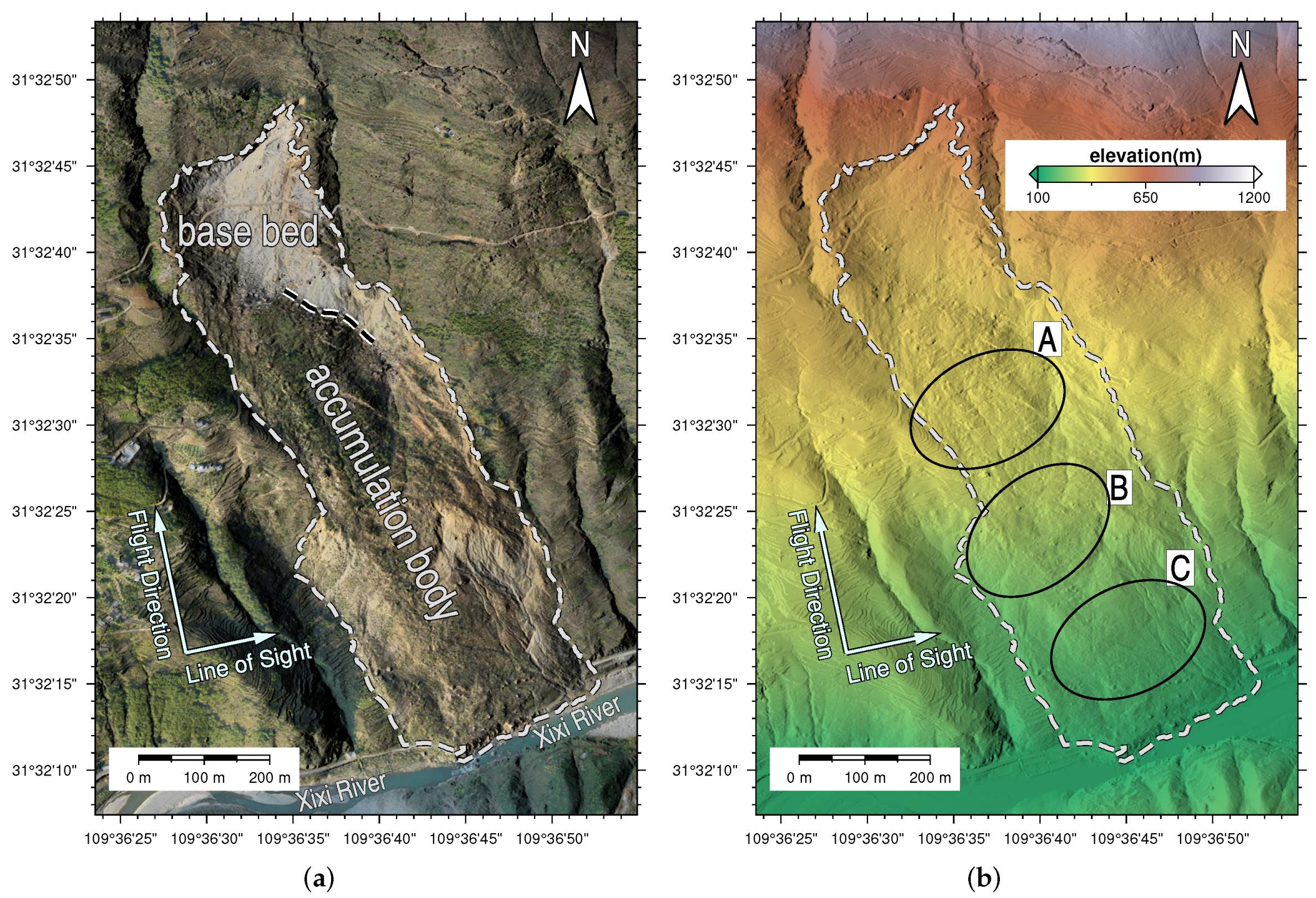
Figure 1.
(a) The airborne true color orthoimage covering the Guang’an Village Landslide. (b) The elevation map at the study area. The white double broken line indicates the boundary between the base bed and the accumulation body to be used as the defined branch cuts in the phase unwrapping process. The white arrows indicate the flight direction and radar line-of-sight direction of the Sentinel-1 data. The three accumulation bodies 1, 2, and 3 are indicated by black ovals marked as A, B, and C, respectively.
The Guang’an Village Landslide occurred on 21 October 2017. The initial landslide deposits have caused the riverbed to uplift, which blocked the river channel for about 160 m in distance over the surface and formed a barrier lake. As can be seen in Figure 1a, the landslide region can be initially classified into two areas based on the morphological features observed from the recent optical images: base bed and accumulation body.
According to the field investigation and longitudinal profile data provided in [1], the landslide region can also be divided into two areas based on their failure characteristics: base bed area and accumulated area. The upper part of the study area is the base bed area and the lower part is the accumulation area. The initial base bed area has a length of about 550 m and a width of 150∼280 m. The average thickness and the volume of the initial base bed area are about 30 m and 360 × 10 m, respectively. The sliding accumulation area is scraped and thrusted by the based bed, forming an accumulation body of about 1100 m in length and 300 m in width. The average thickness and volume of the accumulated area are about 25 m and 825 × 10 m, respectively. In addition to the analysis above, this study roughly divided the study area into four areas with the field survey information provided in [1]: (1) base bed, (2) accumulation body 1, (3) accumulation body 2, and (4) accumulation body 3 (the three accumulation bodies are indicated by black ovals marked as A, B, and C in Figure 1b).
In this study, the analysis is conducted mainly based on three datasets, i.e., the Sentinel-1 SAR data, LiDAR DEM, and the rainfall data. The average daily rainfall data, recorded between 1 January 2018 and 1 April 2022, was collected from the locally installed rainfall gauge near the study area. The ascending track of the C-band Sentinel-1 SAR VV polarized data acquired in the Terrain Observation by Progressive Scans (TOPS) mode were collected for time-series InSAR analysis. A total of 128 Sentinel-1 data acquired between 31 October 2017 and 3 March 2022 (Path 84 Frame 100) were selected for analysis. The flight direction and radar line-of-sight direction (LOS) of the Sentinel-1 data are shown in Figure 1. As can be seen from this figure, the slope direction of the landslide is almost parallel to the flight direction of the Sentinel-1 ascending track. The LOS displacement obtained from TS-InSAR analysis is mainly composed of the landslide displacement in the horizontal and vertical directions. The airborne LiDAR data used in this work were acquired in 2021 to provide high-resolution and up-to-date elevation data for this analysis.
As pointed out in [38], rainfall is one of the most important factors triggering landslide failures. The average daily precipitation data between 1 January and 11 April 2022 were therefore collected from the nearest locally installed gauge (approximately 1.5 km away from the study area). In general, flood season lasts from early April to early October in the study area. According to the rainfall data, the precipitation intensities of 2018, 2019, 2020, and 2021 are 1496.8 mm, 1057.6 mm, 1666.3 mm, and 1712.2 mm, respectively. In total, 6089.2 mm rainfall was recorded during the observation period.
3. Methodology
3.1. Preparation of the Interferogram Stack
In order to generate an image stack for time-series analysis, all Sentinel-1 images have to be co-registered to the same image grid. A primary image acquired on 19 March 2019 was chosen for the generation of a Sentinel-1 image stack. To generate the SAR image stacks, all secondary images are coregistered to the image grid of the primary image. Because of the variations in Doppler centroid frequency in Sentinel-1 TOPS mode, a coregistration accuracy of 1/1000 pixel is required for the interferometric phase error to be negligible between bursts. The enhanced spectral diversity (ESD) method, which is able to achieve such accuracy, was utilized. However, since ESD derives mis-coregistration from the cross-interferometric phase, a fair amount of high coherence pixels are needed at burst overlaps area for the ESD process to achieve the required coregistration accuracy [39]. The high ratio of decorrelated pixels over the landslide region due to the temporal decorrelation could degrade the achieved accuracy from ESD. To avoid this issue, the whole Sentinel-1 scene is processed with the one arc-second Shuttle Radar Topography Mission (SRTM) Digital Elevation Model (DEM) and the Sentinel-1 precise orbits. The purpose of processing the full scene instead of the sub-scene covering only the landslide and nearby areas is to ensure that there are enough high coherence pixels for the ESD process.
Once all SAR images are coregistered to the same grid, a differential interferogram can be formed. In order to ensure an accurate inversion of surface deformation from the time-series InSAR analysis, it is necessary to ensure that the minimum possible decorrelated InSAR pairs are selected. An investigation was conducted prior to the selection of interferometric pairs to obtain the optimal combination of interferometric pairs for time-series analysis. It was found that temporal decorrelation is the dominating decorrelation source after analyzing all possible combinations of interferometric pairs over the study area. There are noticeable outliers that exhibit poor coherence even with a temporal baseline of 24 days. Therefore, the interferometric pairs are selected with the shortest temporal baseline available to guarantee that coherence is preserved in all the image pairs to some extent. One hundred and twenty-seven differential interferograms were generated with respect to the primary image using the conventional two-pass DInSAR approach [40]. A one arc-second SRTM DEM was used to remove the topography phase from the interferograms.
Once the differential interferogram stack is formed, a filtering operation can be conducted to enhance the coherence. Since the location of the deformation zone to be monitored is expected to be small in spatial extent, full-resolution processing is preferred instead of processing with the multi-looked interferogram. The two-sample Kolmogorov–Smirnov (KS) test was carried out to determine the adaptive filtering window, i.e., the statistically homogeneous areas (SHP), for each pixel. The initial searching window of pixels (approximately 0.07 km ) is used here.
3.2. Atmospheric Correction with Masking of the Deforming Area
The differential phase in interferogram k, in the pixel of azimuth and range coordinates from acquired times and is given by:
where is the wavelength of the radar signal and is the LOS displacement between the acquisition times and . The second term in Equation (1) is the phase induced by inaccuracy in the reference DEM. , , , and are the DEM error, mean perpendicular baseline, slant-range distance, and local incidence angle, respectively, between the pixel and the reference point. The third term is induced by the atmospheric inhomogeneities in times and . The last term, , is induced by many factors, including thermal noise, mis-coregistration, inaccurate orbit data, decorrelation, etc.
It is worth noting that the post-failure surface deformation of the Guang’an Village Landslide is highly non-linear, especial within the short time frame. Therefore, the deformation cannot be accurately estimated using the common linear or the seasonal models. For this reason, atmospheric correction must be removed before the spatial phase unwrapping operation to minimize the phase ambiguity problem over the sliding area. In the time-series InSAR analysis, the atmospheric component in Equation (1) is often assumed to be spatially correlated and temporally uncorrelated. Since all InSAR pairs are selected with the shortest possible temporal baseline, the atmospheric phase of each pair can be expressed as:
where is the spatially correlated phase in interferogram k and is the atmospheric phase at acquisition time j for the pixel of azimuth and range coordinates . In this study, is calculated based on the spatial low pass filtering on the wrapped interferogram. It is clear that the design matrix in Equation (2) is rank-deficient. The approach proposed in [41] is adopted here for the atmospheric correction. The interferogram with minimal variance in the interferogram stacks is first obtained and selected and then the selected interferogram is used to calibrate the others based on Equation (2).
Since the post-failure surface deformation is correlated in the spatial domain to some extent, some of the deformation signals can be incorrectly treated as the atmospheric phase using the procedure above. Therefore, refinement of the preliminary atmospheric signal is necessary. The refinement procedure used in this work is as follows: (1) spatial phase unwrapping operation is applied to each interferogram (after the initial atmospheric correction); (2) the accumulated deformation can be obtained by adding up all of the unwrapped interferograms; (3) the deformation area is identified and a mask is created to mask out the sliding area; (4) the atmospheric correction procedure is reapplied with the masked interferograms to estimate the atmospheric phase component; (5) the spatial interpolation is applied to estimate the atmospheric phase at the masked area; (6) the refined atmospheric phases are subtracted from the original differential interferograms.
3.3. Terrain Correction and Spatial Phase Unwrapping
After the atmospheric correction process, the remaining phase in the interferogram is expected to be contributed to mainly by the deformation and DEM error. Since the InSAR pairs are selected with the minimal temporal baseline possible, most pairs are separated by 12 days. Given that the temporal baseline between each pair is relatively short and the landslide deformation is non-linear in time, DEM error can be estimated using the stacking approach [42] without considering the influence of deformation. Once the DEM error is estimated and corrected, spatial phase unwrapping can be applied to the refined interferogram stack for deformation analysis.
Unlike many other TS-InSAR studies, the variation of elevation in the study area is over 700 m within a relatively small spatial extent, i.e., 1.5 km × 0.85 km. The steepness of the slope is up to ∼60. The geometric distortion caused by high elevation and extremely undulating terrain, such as strong layover and foreshortening effects, can induce strong phase distortion. This makes the spatial phase unwrapping process challenging without correcting the terrain effects. Figure 2 shows the amount of geometric distortion observed using the 1 arc-second STRM DEM. The look-up table for geographic-to-radar coordinate projection based on the SRTM DEM and the LiDAR have been generated independently. The amount of geometric distortion is derived by the projected range coordinate difference between the SRTM and the LIDAR look-up tables. These differences can hence be considered to be the projection bias of the SRTM look-up table. It can be clearly observed that largest difference is larger than 20 pixels. Since this study requires processing the data at a full-resolution scale, such a bias will lead to a relatively large distortion in the geographic pattern of the interferometric signals. Although the elevation information obtained from the TS-InSAR analysis can be used to compensate for the DEM error, the variation in the perpendicular baseline of the Sentinel-1 InSAR stack is too small to obtain the required accuracy. In order to deal with this issue, an airborne LIDAR DEM with an expected accuracy of 5 cm is used to assist the phase unwrapping process. The LiDAR DEM with a much higher resolution (0.5 m × 0.5 m) is able to derive the land feature in more detail, which allows the defining of the correct branch-cut to correct the phase unwrapping error, and at the same time provides accurate geolocation information for each pixel. The InSAR interferograms are resampled to a grid with a resolution of 8 m × 8 m based on the LiDAR DEM. The reason for choosing such a resolution is because the number of elements from the map grid and the slant-range grid is approximately the same. Therefore, this allows the phase information to be retained as much as possible without degrading the coherence.
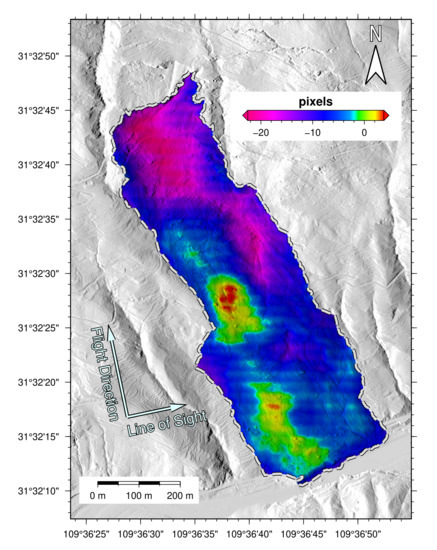
Figure 2.
The projected range coordinate difference between the 1 arc-second SRTM and the LiDAR look-up tables.
Once all interferograms are resampled to the map coordinate, the Goldstein filter [43] is applied to ensure the continuity of the phase data for spatial phase unwrapping. The pixels with temporal coherence, i.e., the sum of complex coherence throughout the stack, larger than 0.75 are considered as coherent pixels for phase unwrapping. The minimum cost network flow phase unwrapping algorithm (MCF) is performed on all the interferograms to derive the unwrapped phase stack [44]. The costs for each flow are derived from the coherence obtained from the space adaptive filter (SHP) in the early stage. The phase unwrapping results are then investigated and the results that contained serious tiling effects [45,46] are identified. Correction is conducted by adding the defined branch cuts to the minimum cost flow network to avoid such an issue. With the data resampled into the map coordinates, branch cuts can be easily defined based on the morphological features from the LiDAR data and the optical images. Figure 3 shows an example of the unwrapped phase in map coordinate with and without the correction using the proposed method. As can be seen in Figure 3a, there is an area with an obvious phase unwrapping error observed in the phase unwrapping result that is obtained without the defined branch cuts between the base bed and the accumulation body (highlighted by the black circle in Figure 3). The phases have integrated from the base bed to the accumulation body at one end and vice versa at the other end. Figure 3b shows the unwrapped result obtained with the defined branch cut between the base bed and the accumulation body (see Figure 1a for the defined branch cut at the boundary). This clearly shows that the phase unwrapping error has been corrected and the phases no longer pass the boundary between the base bed and the accumulation body. This suggests that the proposed method can improve the correctness of the phase unwrapping results.
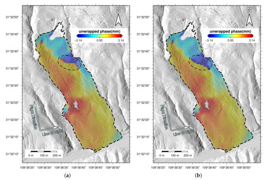
Figure 3.
Unwrapped phase in map coordinates (a) without and (b) with the correction using the proposed method. The area with the obvious phase unwrapping error observed is highlighted by the black circle.
3.4. Time-Series Deformation Analysis
Once the refined interferograms are unwrapped and the DEM error is corrected, network integration in the time domain can be conducted to obtain the time-series deformation information by solving the linear system:
where is the unwrapped deformation phase in refined interferogram k, and is the cumulative deformation along the LOS direction at times corresponding to the acquisition of the secondary images. Finally, a temporal low pass filter with kernel windows of 96 days is applied to the time-series deformation data to remove the decorrelation noise.
4. Results: Deformation Velocity Measured by Time-Series InSAR Analysis
The LOS displacement time-series obtained from the TS-InSAR processing of the 128 Sentinel-1 data are shown in Figure 4 and Figure 5. Figure 6 represents the accumulated displacement. The measurement points (MPs) with red color (positive values) indicate that targets are moving away from the satellite along the LOS direction. On the other hand, the blue color counterparts (negative values) indicate that targets are moving towards the satellite. Figure 4 and Figure 5 show that the study area experienced continuous post-event deformation between 2017 and 2021, after the initial Guang’an Village Landslide in October 2017. Since noticeable deformation is observed in this region, a cumulative deformation map was generated in order to provide a more comprehensive understanding of the spatial distribution of the deformation (Figure 6). A total of around 4700 MPs, covering more than 90% of the landslide area, were obtained. This suggests that single-pixel processing (without multi-looking processing) can effectively avoid the loss of interference signal and maximize the number of MPs in this region. In addition, because the TS-InSAR processing is conducted at the ground distance with the assistance of high-resolution LiDAR DEM, the MPs are more uniformly distributed in the displacement map. This effectively minimized the problem of uneven distribution of MPs due to large topographic relief. According to the TS-InSAR results, it was found that there are two areas, i.e., near the base bed and point 4 (located in accumulation body 2), that experienced strong decorrelation and from which limited MPs can be obtained. Comparing the deformation map with the SAR intensity images and the LiDAR data suggests that the decorrelation near the base bed is mainly due to the strong shortening and layer effect in the region. The main reason for the decorrelation near point 4 in the accumulation body 2 is expected to be the strong SAR shadowing effect.
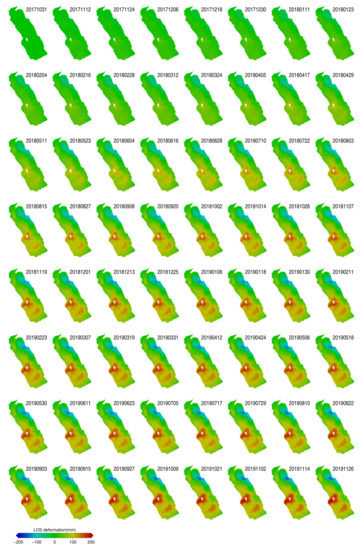
Figure 4.
LOS displacement time-series maps for the Guang’an Village Landslide at the 128 Sentinel-1 acquisition date, referring to the first SAR image acquired on 31 October 2017 (from 31 October 2017 to 26 November 2019). The number at the upper right of each subplot represents the image acquisition date (in yyyymmdd format).
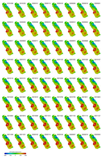
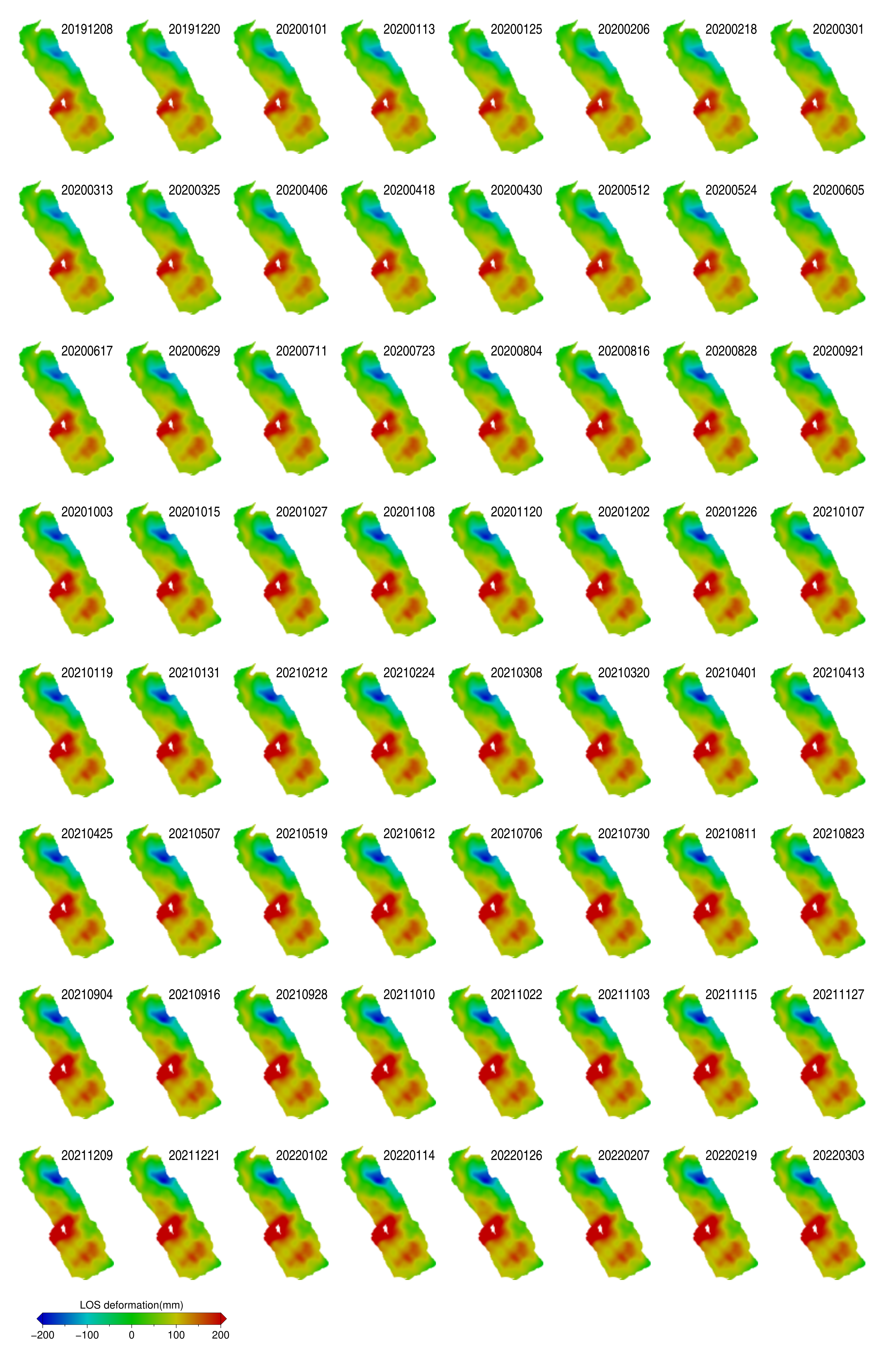
Figure 5.
LOS displacement time-series maps for the Guang’an Village Landslide at the 128 Sentinel-1 acquisition date, referring to the first SAR image acquired on 31 October 2017 (from 8 December 2019 to 3 March 2022). The number at the upper right of each subplot represents the image acquisition date (in yyyymmdd format).

Figure 6.
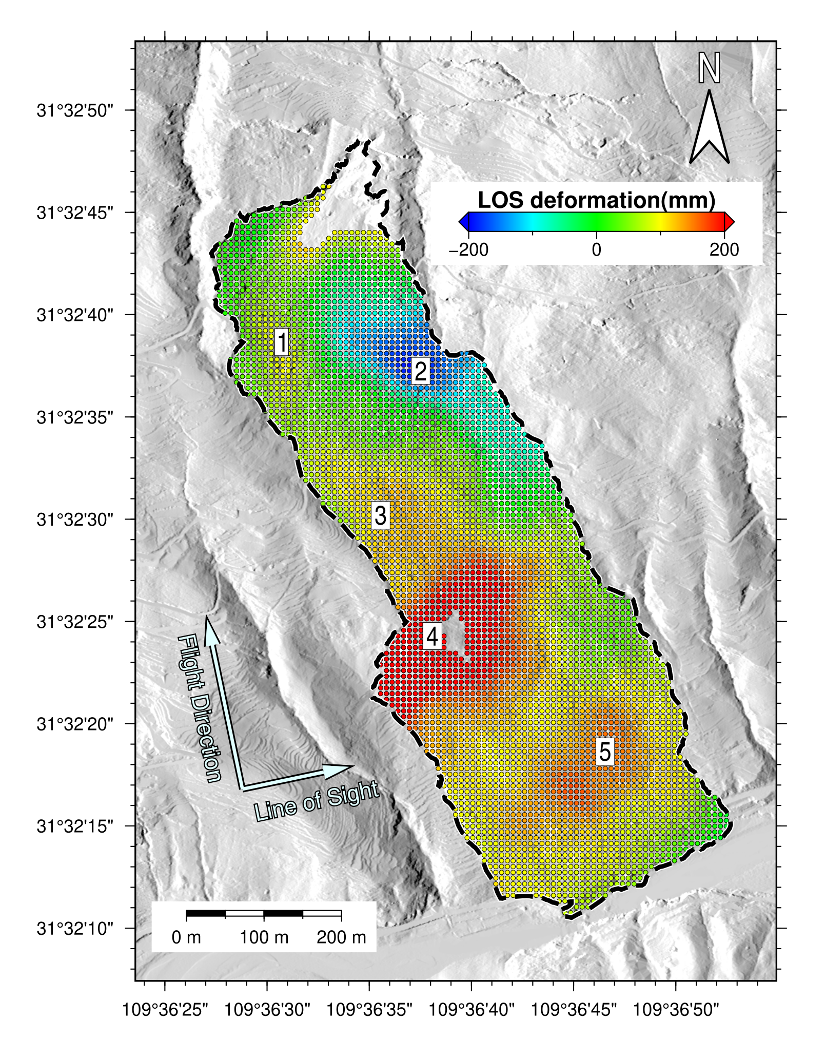
Cumulative LOS displacement between 31 October 2017 and 3 March 2022 for the Guang’an Village Landslide. The numbers 1 to 5 indicate the five active deformation zones for Figure 7.
As shown in Figure 6, there are five active deformation zones. The maximum cumulative LOS deformations observed at the areas near the five points are approximately 80 mm, 80 mm, −200 mm, 200 mm, and 150 mm, respectively, of which point 2 has the maximum accumulated LOS deformation. As mentioned in the previous section, the direction of the flight path is parallel to the main sliding direction. Therefore, all points except for point 2 are experiencing the ground surface moving away from the satellite, where InSAR-derived deformation in these regions is expected mainly in the vertical direction. On the other hand, point 2 is experiencing the ground surface moving towards the satellite, suggesting that the InSAR-derived deformation is expected mainly in horizontal displacement perpendicular to the flight direction.
Figure 7 shows the deformation trend of MPs with the highest displacement from each of the five active deformation zones. It can be seen that all the five MPs have ladder-like deformation characteristics, but have a different degree of correlation with rainfall.
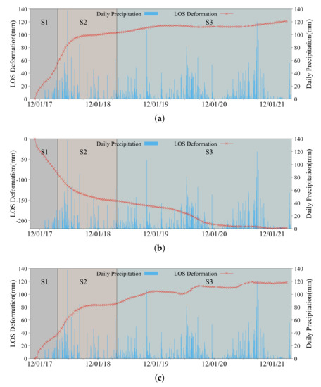
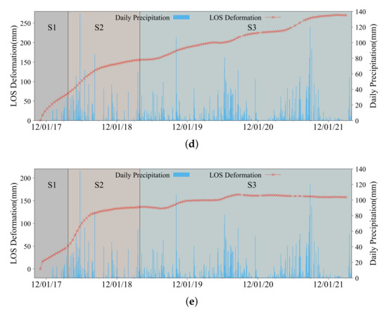
Figure 7.
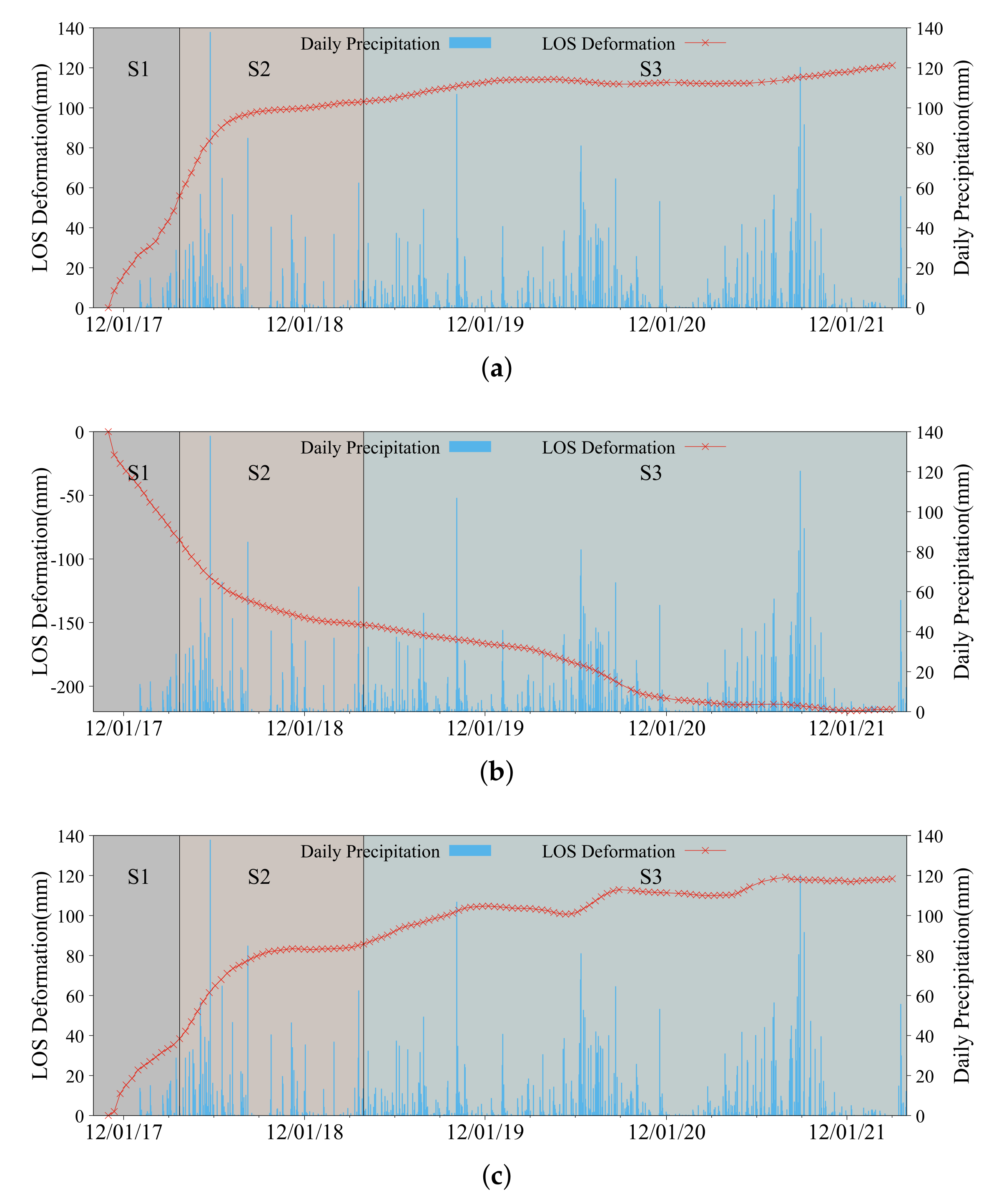
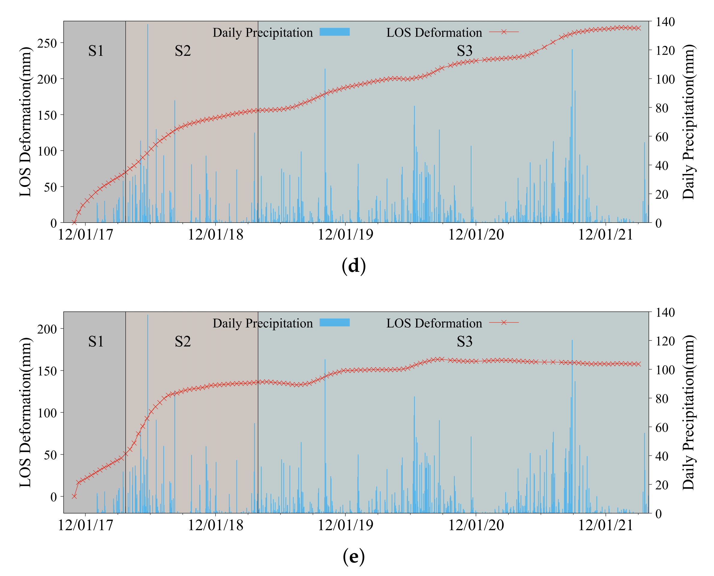
Time-series of the post-event displacement and rainfall for selected MPs from the five active deformation zones: (a) point 1, (b) point 2, (c) point 3, (d) point 4, (e), and point 5, from the cumulative displacement map (Figure 6). The three landslide movement stages S1, S2, and S3 in Figure 8 are highlighted by three-color backgrounds in the time-series plot.
5. Discussion
5.1. Temporal–Spatial Evolution of the Post-Event Deformation of the Guang’an Village Landslide
In this section, the spatial-temporal evolution of the post-event slope stability at the active deformation zones are analyzed. As can be seen from the displacement time-series in Figure 7, during the observation period, point 3 and 4 show an obvious periodic “acceleration-creep” deformation pattern before and after the flood season every year, indicating that the deformation trends at these active deformation zones are strongly correlated with the rainfall in the flood season. Apart from the two points mentioned, the acceleration of deformation is strongly correlated to the rainfall intensity at point 5 from 2018 to 2020. However, once the accumulated deformation reached its peak after the flood season in 2020, the accumulated deformation remained stable even under the action of the rainfall during the flood season in 2021. Continuous deformation has been observed at point 1 since the initial landslide incident, but the deformation rate significantly decreased after the flood season in 2018. Even though the point continues to deform, the acceleration in deformation observed during flood season rainfall is relatively low and the correlation between the deformation and rainfall during the flood season is decreased significantly compared with that in 2018. Compared to the rest of the MPs, point 2 shows a unique continuous deformation trend with an opposite sign (moving towards the satellite). As discussed previously, the deformation at point 2 is mainly in horizontal displacement in the direction perpendicular to the flight direction. Rapid deformation was observed after the initial landslide incident. However, the rate of deformation decreased significantly along with the weakening of rainfall after the flood season in 2018. Because the amount of rainfall in the flood season of 2019 was lower compared to the other years, the deformation rate at point 2 was relatively stable after the flood season of 2018 until the beginning of the flood season in 2020. An obvious acceleration in deformation was observed under the action of rainfall in the flood season of 2020. However, although the peak daily rainfall intensity was higher during the flood season in 2021 than in 2020, only a small “acceleration-creep” deformation trend was observed.
According to [47], the landslide movement can be classified into four stages: (1) a pre-failure stage including a deformation process leading to failure; (2) the onset of failure characterized by the formation of a continuous shear surface through the entire soil mass; (3) a post-failure stage starting from failure until the mass stops; (4) a reactivation stage when sliding occurs on a pre-existing shear surface. By taking the four landslide movement stages proposed by [47] into account, the temporal evolution of the post-event deformation at the five selected MPs is classified into three stages here based on correlation analysis between the change in deformation rate and rainfall: (1) post-failure stage (S1: until 24 March 2018), (2) post-failure and reactivation stage (S2: between 25 March 2018 and 31 March 2019), and (3) reactivation stage (S3: after 31 March 2019). The criteria used for such a classification can be summarized as follows. (1) The flood season over the Wuxi County starts from the beginning of April. (2) According to Figure 7, the displacement observed on each point during 2018 is clearly larger than that observed during 2019, 2020, and 2021. (3) For the cases of point 1 and point 5, the deformation evaluations generally remain stable after 2018. The three landslide movement stages S1, S2, and S3 at the five selected MPs are highlighted in Figure 7.
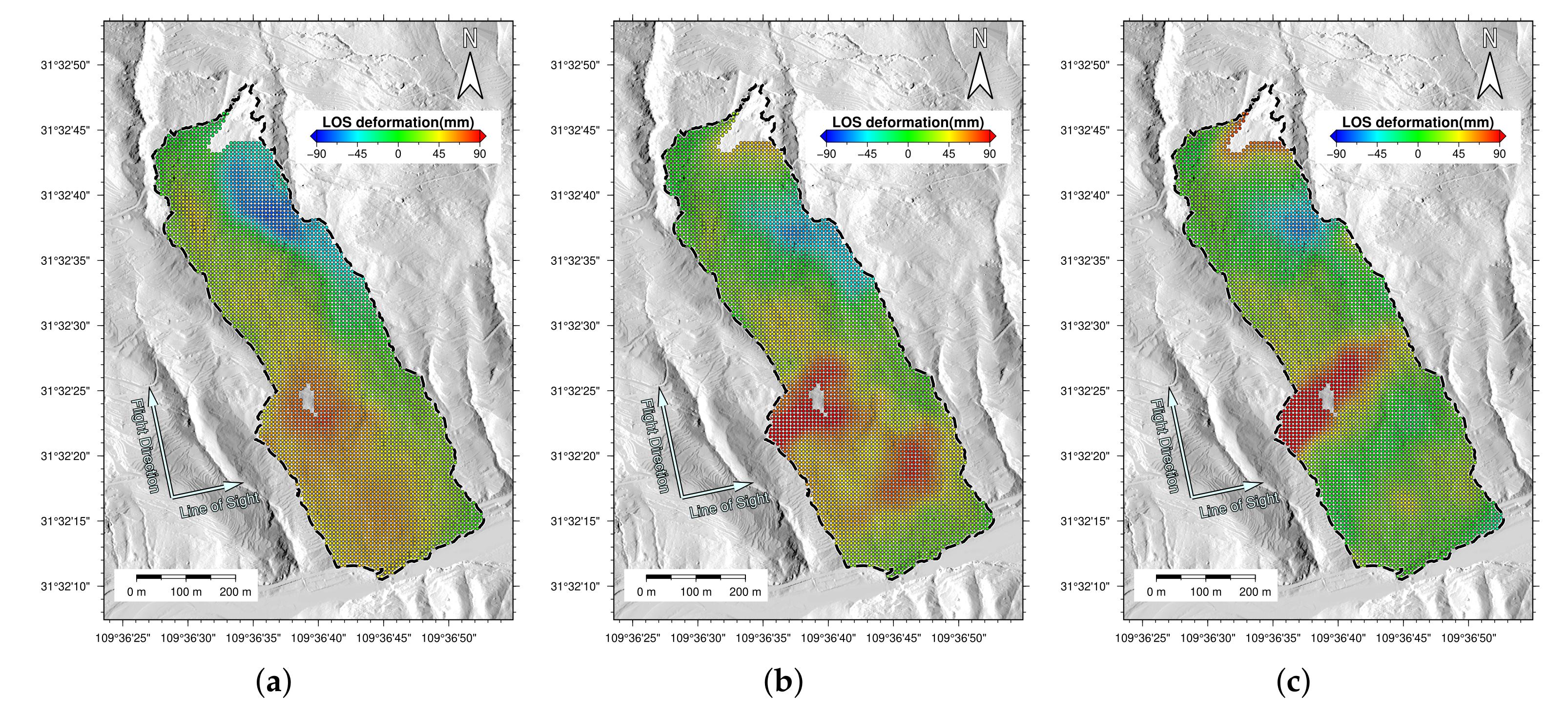
In order to analyze the spatial distribution of deformations at the three stages, the cumulative deformation corresponding to the three stages is computed (Figure 8). As can be seen in Figure 8, the spatial extent of the deformation areas has gradually reduced and most of the affected area was stabilized from S1 to S3. During stage S1, the deformation was mainly concentrated in the active deformation zones point 2 and point 4. The non-active deformation areas were mainly affected by horizontal movement at the active deformation zones point 2 and by surface movement in slip directions at the active deformation zone point 4. During stage S2, the deformation was mainly concentrated in the active deformation zones point 4 and point 5. The deformation in the landslide area tended to be stable. During stage S3, the front edge of the landslide area tended to be stable. However, noticeable deformation was observed in the active deformation zones point 2 and point 4, and the spatial extent of the deformation zones gradually extended from the west boundary of the landslide to the east boundary.

Figure 8.
The cumulative LOS displacement maps of the three landslide movement stages: (a) S1: post-failure stage, (b) S2: post-failure + reactivation stage, and (c) S3: reactivation stage.
5.2. Deformation Mechanism Analysis and Risk Evaluation of the Guang’an Village Landslide Area
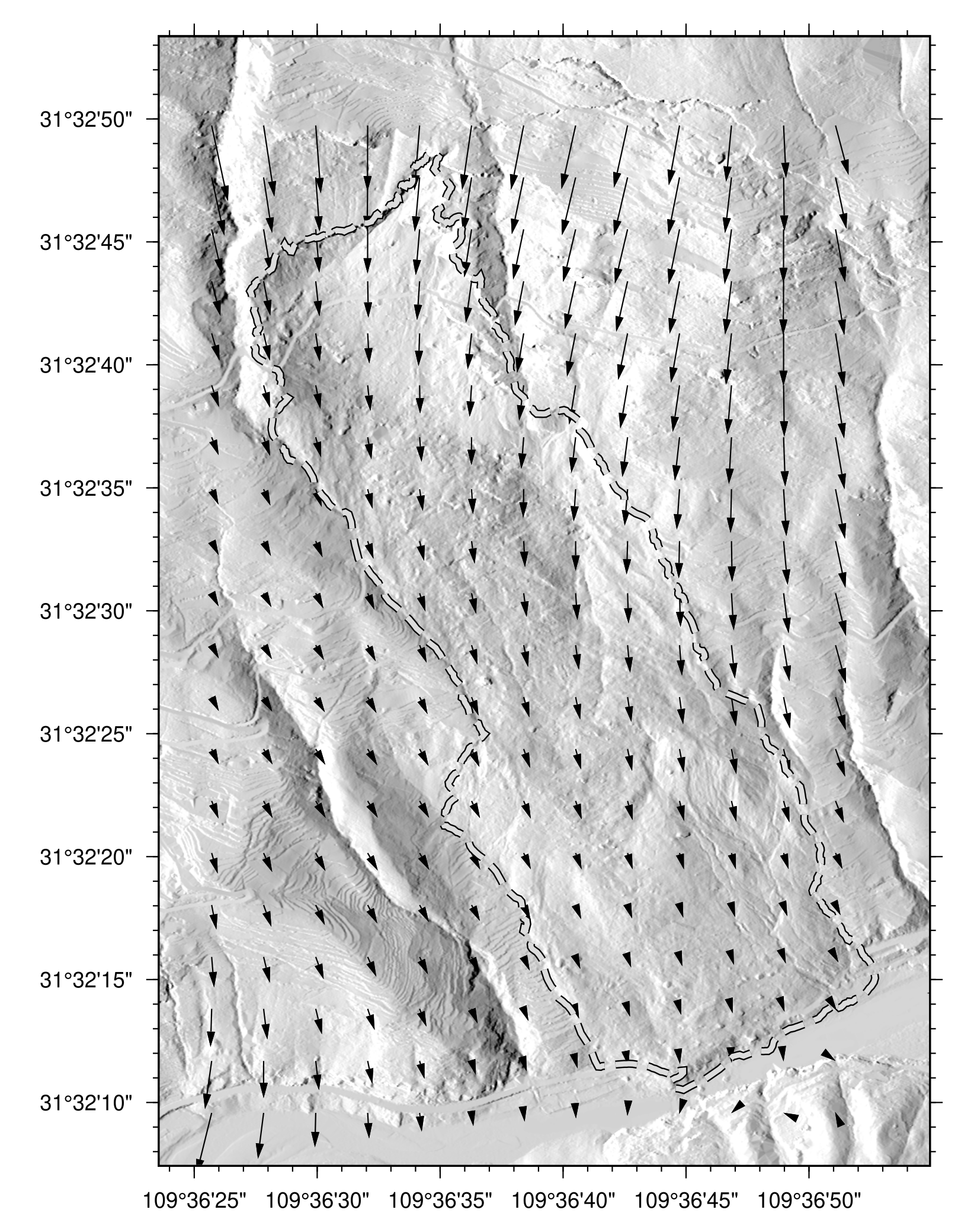
According to the cumulative displacement at the reactivation stage (Figure 8c), there are two zones (points 2 and 4) in the study area where intensive deformation was observed, which may become the potential trigger source for the secondary landslide. Based on the above analysis, it was found that there is a clear difference between the deformation phenomenon in active deformation zone point 2 (source area) and the rest of the deformation zones. To investigate the reason why the deformation trend was opposite in point 2, the gravity trend direction over the region was computed based on the least square solution of the eight-neighbor elevation difference from the high-precision LiDAR DEM (Figure 9). It can be seen that there is a certain angle between the gravity trend direction of the active deformation zone point 2 and the main sliding direction of the slope. This may lead to the abnormal deformation trend in the zone. In addition, by analyzing the study area and its surroundings using the LiDAR data, it was found that there is a long crack appearing at the north-east of the study area (Figure 10), which suggests that it is highly likely there is deformation occurring in that area. This finding has been verified with the field investigation, and the slope instability in that area is named the Yaodunzi Landslide.

Figure 9.
The quiver plot of the gravity trend direction for the Guang’an Village Landslide and surroundings.
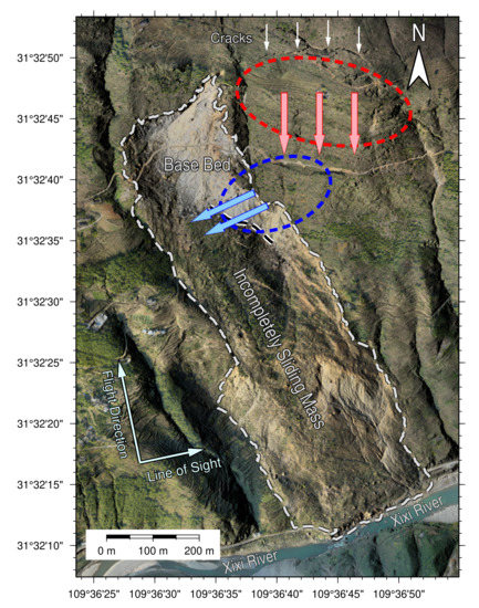
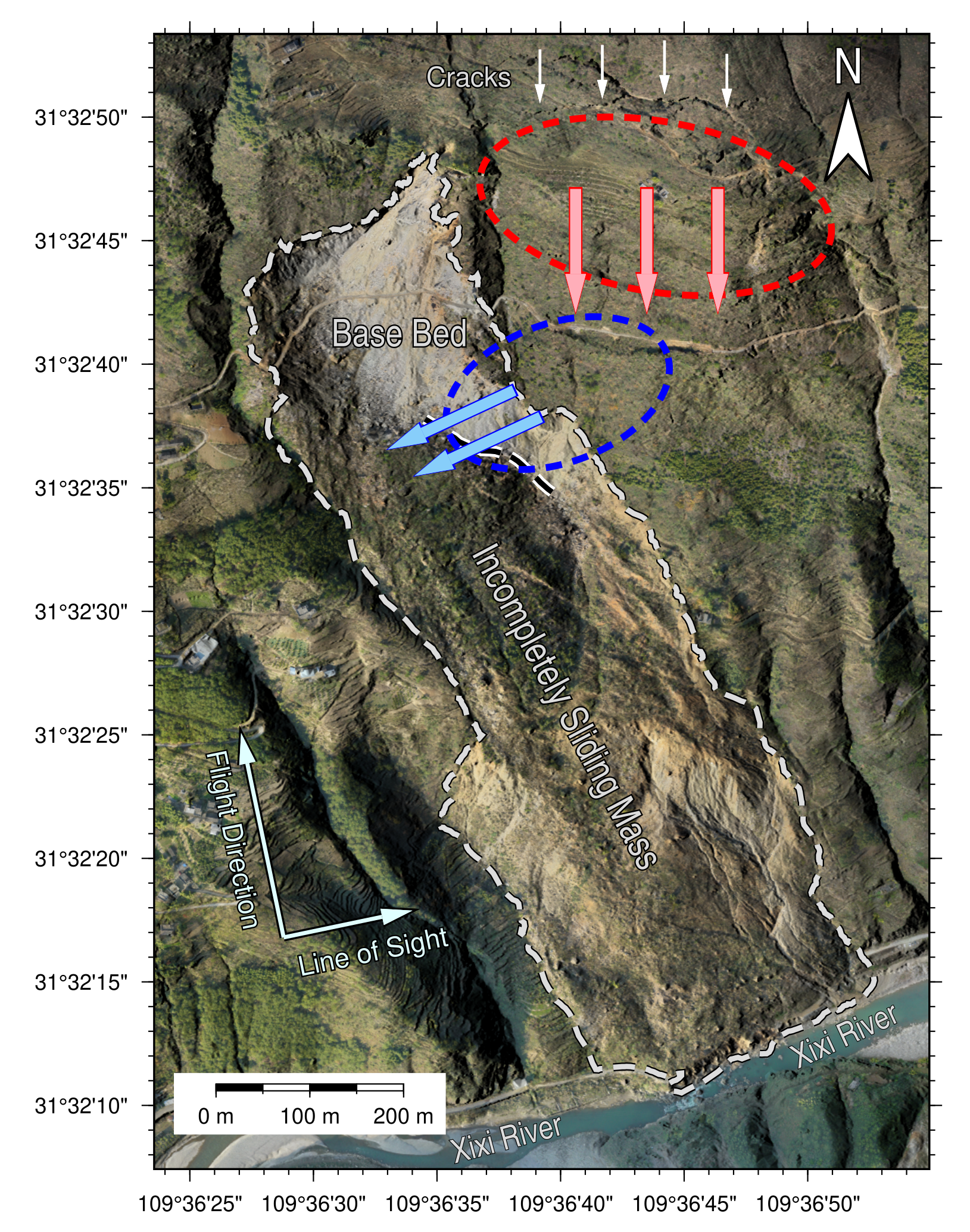
Figure 10.
The effect of the Yaodunzi Landslide on the active deformation zone point 2. The arrow indicates the force induced by the Yaodunzi landslide. The red and blue arrows represent the indirect force and direct force, respectively, to the active deformation zone point 2. The white arrows show the location of the cracks at the rear edge of Yaodunzi landslide.
As the Yaodunzi Landslide area moves in the slope direction, it can induce the pressure on the accumulation body in the Guang’an Village Landslide, leading to horizontal displacement perpendicular to the main sliding direction (moving towards the satellite) in the active deformation zone (Figure 10). In fact, the active deformation zone where point 2 is located becomes the main anti-sliding section of the Yaodunzi Landslide. The anti-sliding force in this area is mainly composed of two parts: (1) the friction between the accumulation body and the sliding bed in this area; (2) the lower area acting as the anti-sliding force to this area. According to the profile (see [1]), since the initial Guang’an Village Landslide, the thickness of the accumulation layer in this area is relatively shallow and the normal stress of the sliding bed is relatively limited. Therefore, the contribution of the anti-sliding force from the second part is likely to be larger than the first part.
This can also be observed in the deformation time-series of the active deformation zones point 3, point 4, and point 5 (Figure 7) that the deformation trends of these zones are relatively synchronous. However, the InSAR results in Figure 8c show that the cumulative surface deformation in S3 stage is highest at the accumulation body 2 (where point 4 is located). Since the sliding direction of the landslide is almost perpendicular to the Sentinel-1 LOS direction, the actual deformation in the accumulation 2 region may be much larger than the InSAR LOS displacement values. Based on the above analysis, the Guang’an Village Landslide may have two chain failure modes under extreme rainfall conditions: (1) rainfall infiltrates from the cracks at the rear edge of the Yaodunzi Landslide under heavy rainfall, resulting in the reduction of the anti-sliding force from the sliding soil of the Yaodunzi Landslide. The anti-sliding force from active deformation zone point 2 then can no longer maintain the stability of the Yaodunzi landslide, causing a failure of the slope; (2) the accumulation 2 region continues to deform under the heavy rainfall and the continuous deformation in this area leads to the slope instability of accumulation 1 region, and eventually to the slope failure of the Yaodunzi Landslide.
6. Concluding Remarks
This study developed an approach, based on the conventional TS-InSAR method, to monitor the post-event deformation of the Guang’an Village Landslide, which integrates the LiDAR data into the TS-InSAR processing chain. This approach has two main features: (1) a multi-looking process is not conducted to minimize the loss of interferometric signal due to the down-sampling issue; (2) TS-InSAR analysis is conducted on the ground distance, which minimized the influence of geometric distortion in slant-range coordinates on the geocoded deformation results. This allows the spatial distribution of measurement points to be in line with prior geological knowledge, and hence prior knowledge can be applied to assist the spatial phase unwrapping process. A total of 128 Sentinel-1 SAR images, acquired from October 2017 to March 2022, were analyzed to obtain the long-term evolution of the post-event deformation of the landslide area. The InSAR-derived deformation information, LiDAR DEM, and the rainfall data were jointly used to analyze and explore the deformation characteristics of the study area. It was found that: (1) the study area tends to be stable in general, but there are two areas that continue to suffer from deformation due to rainfall in the flood season; (2) the post-event deformation between October 2017 and March 2022 can be divided into three main stages: the post-failure stage (October 2017 to March 2018), the post-failure and reactivation stage (March 2018 to March 2019), and the reactivation stage (March 2019 to March 2022); (3) the results show that the study area can be further divided into four main areas: base bed, accumulation body 1, accumulation body 2, and accumulation body 3. Among the four areas, it is observed that there are signs of abnormal accumulation of lateral deformation at the trailing edge of accumulation 1 area. A possible reason for such deformation is that the upper part of accumulation 1 is suffering from downward movement and compression from another landslide (Yaodunzi Landslide), resulting in lateral deformation occurring at the upper part of the accumulation 1 area; (4) although the study area is currently in the reactivation stage, active deformation zones have been found in both accumulation body 1 and accumulation body 2 areas. These active deformation zones are strongly correlated to rainfall intensity in the flood season. These two deformation zones may become the origin of a secondary landslide triggered by heavy rainfall in the future. On-going monitoring of these areas is therefore essential for the detection and early warning of further failure and for planning an emergency response.
Author Contributions
Conceptualization, K.Z. and F.G.; methodology, K.Z. and L.L.; software, K.Z. and L.L.; validation, F.G. and A.H.-M.N.; formal analysis, K.Z. and P.L.; investigation, L.L., A.H.-M.N., and P.L.; resources, K.Z. and A.H.-M.N.; data curation, K.Z., F.G., and L.L.; writing—original draft preparation, F.G.; writing—review and editing, K.Z.; visualization, A.H.-M.N. and P.L.; supervision, K.Z.; project administration, K.Z.; funding acquisition, K.Z. All authors have read and agreed to the published version of the manuscript.
Funding
This research was funded by the National Natural Science Foundation of China (Grant No. 42074034) and the Program for Guangdong Introducing Innovative and Entrepreneurial Teams (2019ZT08L213).
Institutional Review Board Statement
Not applicable.
Informed Consent Statement
Not applicable.
Data Availability Statement
Sentinel-1 data were analyzed in this study. This data can be found here: https://asf.alaska.edu/ (accessed on 29 March 2022).
Acknowledgments
The authors are very grateful to the European Space Agency for providing Sentinel-1 data.
Conflicts of Interest
The authors declare no conflict of interest.
References
- Wang, L.; Yin, Y.; Huang, B.; Zhang, Z.; Wei, Y. Formation and characteristics of Guang’an Village landslide in Wuxi, Chongqing, China. Landslides 2019, 16, 127–138. [Google Scholar] [CrossRef]
- Bamler, R.; Hartl, P. Synthetic aperture radar interferometry. Inverse Probl. 1998, 14, R1. [Google Scholar] [CrossRef]
- Gabriel, A.K.; Goldstein, R.M.; Zebker, H.A. Mapping small elevation changes over large areas: Differential radar interferometry. J. Geophys. Res. Solid Earth 1989, 94, 9183–9191. [Google Scholar] [CrossRef]
- Massonnet, D.; Feigl, K.L. Radar interferometry and its application to changes in the Earth’s surface. Rev. Geophys. 1998, 36, 441–500. [Google Scholar] [CrossRef] [Green Version]
- Rosen, P.A.; Hensley, S.; Joughin, I.R.; Li, F.K.; Madsen, S.N.; Rodriguez, E.; Goldstein, R.M. Synthetic aperture radar interferometry. Proc. IEEE 2000, 88, 333–382. [Google Scholar] [CrossRef]
- Simons, M.; Rosen, P. Interferometric synthetic aperture radar geodesy. In Treatise on Geophysics-Geodesy; Elsevier: Amsterdam, The Netherlands, 2007. [Google Scholar]
- Ferretti, A.; Prati, C.; Rocca, F. Permanent scatterers in SAR interferometry. IEEE Trans. Geosci. Remote Sens. 2001, 39, 8–20. [Google Scholar] [CrossRef]
- Berardino, P.; Fornaro, G.; Lanari, R.; Sansosti, E. A new algorithm for surface deformation monitoring based on small baseline differential SAR interferograms. IEEE Trans. Geosci. Remote Sens. 2002, 40, 2375–2383. [Google Scholar] [CrossRef] [Green Version]
- Mora, O.; Lanari, R.; Mallorqui, J.J.; Berardino, P.; Sansosti, E. A new algorithm for monitoring localized deformation phenomena based on small baseline differential SAR interferograms. IEEE Int. Geosci. Remote Sens. Symp. 2002, 2, 1237–1239. [Google Scholar]
- Ferretti, A.; Fumagalli, A.; Novali, F.; Prati, C.; Rocca, F.; Rucci, A. A new algorithm for processing interferometric data-stacks: SqueeSAR. IEEE Trans. Geosci. Remote Sens. 2011, 49, 3460–3470. [Google Scholar] [CrossRef]
- Dong, J.; Zhang, L.; Tang, M.; Liao, M.; Xu, Q.; Gong, J.; Ao, M. Mapping landslide surface displacements with time series SAR interferometry by combining persistent and distributed scatterers: A case study of Jiaju landslide in Danba, China. Remote Sens. Environ. 2018, 205, 180–198. [Google Scholar] [CrossRef]
- Blanco-Sanchez, P.; Mallorquí, J.J.; Duque, S.; Monells, D. The coherent pixels technique (CPT): An advanced DInSAR technique for nonlinear deformation monitoring. In Earth Sciences and Mathematics; Birkhäuser Verlag AG: Basel, Switzerland, 2008; pp. 1167–1193. [Google Scholar]
- Blanco, P.; Mallorqui, J.; Duque, S.; Navarrete, D. Advances on DInSAR with ERS and ENVISAT data using the coherent pixels technique (CPT). In Proceedings of the 2006 IEEE International Symposium on Geoscience and Remote Sensing, Denver, CO, USA, 31 July–4 August 2006; pp. 1898–1901. [Google Scholar]
- Ng, A.H.M.; Ge, L.; Li, X.; Zhang, K. Monitoring ground deformation in Beijing, China with persistent scatterer SAR interferometry. J. Geod. 2012, 86, 375–392. [Google Scholar] [CrossRef]
- Ge, L.; Ng, A.H.M.; Li, X.; Abidin, H.Z.; Gumilar, I. Land subsidence characteristics of Bandung Basin as revealed by ENVISAT ASAR and ALOS PALSAR interferometry. Remote Sens. Environ. 2014, 154, 46–60. [Google Scholar] [CrossRef]
- Ng, A.H.M.; Ge, L.; Li, X. Assessments of land subsidence in the Gippsland Basin of Australia using ALOS PALSAR data. Remote Sens. Environ. 2015, 159, 86–101. [Google Scholar] [CrossRef]
- Werner, C.; Wegmuller, U.; Strozzi, T.; Wiesmann, A. Interferometric point target analysis for deformation mapping. In Proceedings of the IGARSS 2003. 2003 IEEE International Geoscience and Remote Sensing Symposium. Proceedings (IEEE Cat. No. 03CH37477), Toulouse, France, 21–25 July 2003; Volume 7, pp. 4362–4364. [Google Scholar]
- Biggs, J.; Wright, T.; Lu, Z.; Parsons, B. Multi-interferogram method for measuring interseismic deformation: Denali Fault, Alaska. Geophys. J. Int. 2007, 170, 1165–1179. [Google Scholar] [CrossRef] [Green Version]
- Wang, H.; Wright, T.J.; Yu, Y.; Lin, H.; Jiang, L.; Li, C.; Qiu, G. InSAR reveals coastal subsidence in the Pearl River Delta, China. Geophys. J. Int. 2012, 191, 1119–1128. [Google Scholar] [CrossRef] [Green Version]
- Costantini, M.; Falco, S.; Malvarosa, F.; Minati, F.; Trillo, F. Method of persistent scatterer pairs (PSP) and high resolution SAR interferometry. In Proceedings of the 2009 IEEE International Geoscience and Remote Sensing Symposium, Cape Town, South Africa, 12–17 July 2009; Volume 3, pp. III-904–III-907. [Google Scholar]
- Hooper, A. A multi-temporal InSAR method incorporating both persistent scatterer and small baseline approaches. Geophys. Res. Lett. 2008, 35. [Google Scholar] [CrossRef] [Green Version]
- Hooper, A.; Segall, P.; Zebker, H. Persistent scatterer interferometric synthetic aperture radar for crustal deformation analysis, with application to Volcán Alcedo, Galápagos. J. Geophys. Res. Solid Earth 2007, 112. [Google Scholar] [CrossRef] [Green Version]
- Kampes, B.M. Radar Interferometry; Springer: Dordrecht, The Netherlands, 2006; Volume 12. [Google Scholar]
- Zhang, L.; Ding, X.; Lu, Z. Ground settlement monitoring based on temporarily coherent points between two SAR acquisitions. ISPRS J. Photogramm. Remote Sens. 2011, 66, 146–152. [Google Scholar] [CrossRef]
- Zhang, L.; Lu, Z.; Ding, X.; Jung, H.s.; Feng, G.; Lee, C.W. Mapping ground surface deformation using temporarily coherent point SAR interferometry: Application to Los Angeles Basin. Remote Sens. Environ. 2012, 117, 429–439. [Google Scholar] [CrossRef]
- Dong, J.; Liao, M.; Xu, Q.; Zhang, L.; Tang, M.; Gong, J. Detection and displacement characterization of landslides using multi-temporal satellite SAR interferometry: A case study of Danba County in the Dadu River Basin. Eng. Geol. 2018, 240, 95–109. [Google Scholar] [CrossRef]
- He, K.; Li, J.; Li, B.; Zhao, Z.; Zhao, C.; Gao, Y.; Liu, Z. The Pingdi landslide in Shuicheng, Guizhou, China: Instability process and initiation mechanism. Bull. Eng. Geol. Environ. 2022, 81, 1–17. [Google Scholar] [CrossRef]
- Shi, X.; Xu, Q.; Zhang, L.; Zhao, K.; Dong, J.; Jiang, H.; Liao, M. Surface displacements of the Heifangtai terrace in Northwest China measured by X and C-band InSAR observations. Eng. Geol. 2019, 259, 105181. [Google Scholar] [CrossRef]
- Zhang, J.; Zhu, W.; Cheng, Y.; Li, Z. Landslide Detection in the Linzhi–Ya’an Section along the Sichuan–Tibet Railway Based on InSAR and Hot Spot Analysis Methods. Remote Sens. 2021, 13, 3566. [Google Scholar] [CrossRef]
- Zhou, C.; Cao, Y.; Yin, K.; Wang, Y.; Shi, X.; Catani, F.; Ahmed, B. Landslide characterization applying sentinel-1 images and InSAR technique: The muyubao landslide in the three Gorges Reservoir Area, China. Remote Sens. 2020, 12, 3385. [Google Scholar] [CrossRef]
- Dong, J.; Zhang, L.; Li, M.; Yu, Y.; Liao, M.; Gong, J.; Luo, H. Measuring precursory movements of the recent Xinmo landslide in Mao County, China with Sentinel-1 and ALOS-2 PALSAR-2 datasets. Landslides 2018, 15, 135–144. [Google Scholar] [CrossRef]
- Intrieri, E.; Raspini, F.; Fumagalli, A.; Lu, P.; Del Conte, S.; Farina, P.; Allievi, J.; Ferretti, A.; Casagli, N. The Maoxian landslide as seen from space: Detecting precursors of failure with Sentinel-1 data. Landslides 2018, 15, 123–133. [Google Scholar] [CrossRef] [Green Version]
- Kuang, J.; Ng, A.H.M.; Ge, L. Displacement Characterization and Spatial-Temporal Evolution of the 2020 Aniangzhai Landslide in Danba County Using Time-Series InSAR and Multi-Temporal Optical Dataset. Remote Sens. 2022, 14, 68. [Google Scholar] [CrossRef]
- Li, M.; Zhang, L.; Dong, J.; Tang, M.; Shi, X.; Liao, M.; Xu, Q. Characterization of pre-and post-failure displacements of the Huangnibazi landslide in Li County with multi-source satellite observations. Eng. Geol. 2019, 257, 105140. [Google Scholar] [CrossRef]
- Lu, Z.; Kim, J. A Framework for Studying Hydrology-Driven Landslide Hazards in Northwestern US Using Satellite InSAR, Precipitation and Soil Moisture Observations: Early Results and Future Directions. GeoHazards 2021, 2, 17–40. [Google Scholar] [CrossRef]
- Ciampalini, A.; Raspini, F.; Lagomarsino, D.; Catani, F.; Casagli, N. Landslide susceptibility map refinement using PSInSAR data. Remote Sens. Environ. 2016, 184, 302–315. [Google Scholar] [CrossRef]
- Scaioni, M.; Longoni, L.; Melillo, V.; Papini, M. Remote sensing for landslide investigations: An overview of recent achievements and perspectives. Remote Sens. 2014, 6, 9600–9652. [Google Scholar] [CrossRef] [Green Version]
- Sun, D.; Gu, Q.; Wen, H.; Shi, S.; Mi, C.; Zhang, F. A Hybrid Landslide Warning Model Coupling Susceptibility Zoning and Precipitation. Forests 2022, 13, 827. [Google Scholar] [CrossRef]
- Iglesias, R.; Mallorqui, J.J.; López-Dekker, P. DInSAR pixel selection based on sublook spectral correlation along time. IEEE Trans. Geosci. Remote Sens. 2013, 52, 3788–3799. [Google Scholar] [CrossRef]
- Massonnet, D.; Rossi, M.; Carmona, C.; Adragna, F.; Peltzer, G.; Feigl, K.; Rabaute, T. The displacement field of the Landers earthquake mapped by radar interferometry. Nature 1993, 364, 138–142. [Google Scholar] [CrossRef]
- Ng, A.H.M.; Ge, L.; Yan, Y.; Li, X.; Chang, H.C.; Zhang, K.; Rizos, C. Mapping accumulated mine subsidence using small stack of SAR differential interferograms in the Southern coalfield of New South Wales, Australia. Eng. Geol. 2010, 115, 1–15. [Google Scholar] [CrossRef]
- Zhang, K.; Li, Z.; Meng, G.; Dai, Y. A very fast phase inversion approach for small baseline style interferogram stacks. ISPRS J. Photogramm. Remote Sens. 2014, 97, 1–8. [Google Scholar] [CrossRef]
- Goldstein, R.M.; Werner, C.L. Radar interferogram filtering for geophysical applications. Geophys. Res. Lett. 1998, 25, 4035–4038. [Google Scholar] [CrossRef] [Green Version]
- Costantini, M. A novel phase unwrapping method based on network programming. IEEE Trans. Geosci. Remote Sens. 1998, 36, 813–821. [Google Scholar] [CrossRef]
- Chen, C.W.; Zebker, H.A. Two-dimensional phase unwrapping with use of statistical models for cost functions in nonlinear optimization. JOSA A 2001, 18, 338–351. [Google Scholar] [CrossRef] [PubMed] [Green Version]
- Zhang, K.; Ge, L.; Hu, Z.; Ng, A.H.M.; Li, X.; Rizos, C. Phase unwrapping for very large interferometric data sets. IEEE Trans. Geosci. Remote Sens. 2011, 49, 4048–4061. [Google Scholar] [CrossRef]
- Leroueil, S. Geotechnics of slopes before failure. Landslides Eval. Stab. Lacerda Ehrlich Fontoura Sayao (Eds) 2004, 1, 863–884. [Google Scholar]


Publisher’s Note: MDPI stays neutral with regard to jurisdictional claims in published maps and institutional affiliations. |
© 2022 by the authors. Licensee MDPI, Basel, Switzerland. This article is an open access article distributed under the terms and conditions of the Creative Commons Attribution (CC BY) license (https://creativecommons.org/licenses/by/4.0/).