Article

An Ecosystem Services-Centric Land Use and Land Cover Classification for a Subbasin of the Tampa Bay Watershed

by
John J. Lagrosa IV
1,*,†,
Wayne C. Zipperer
2 and
Michael G. Andreu
3
1
Center for Urban Environmental Research and Education (CUERE), University of Maryland, Baltimore County, 1000 Hilltop Circle, TRC, Rm. 149, Baltimore, MD 21250, USA
2
USDA Forest Service, Southern Research Station 4952, Gainesville, FL 32625, USA
3
School of Forest, Fisheries, and Geomatics Sciences, University of Florida, Gainesville, FL 32611, USA
*
Author to whom correspondence should be addressed.
This manuscript is part of a Ph.D. dissertation by the first author, available online at https://ufdc.ufl.edu/.
Forests 2022, 13(5), 745; https://doi.org/10.3390/f13050745
Submission received: 26 April 2022 / Revised: 9 May 2022 / Accepted: 10 May 2022 / Published: 11 May 2022
(This article belongs to the Special Issue Designing Future Urban Forests)

Abstract

:
Land-use and land-cover (LULC) change is a primary driver of terrestrial carbon release, often through the conversion of forest into agriculture or expansion of urban areas. Classification schemes are a key component of landscape analyses. This study creates a novel LULC classification scheme by incorporating ecological data to redefine classes of an existing LULC classification based on variation in above-ground tree carbon. A tree inventory was conducted for 531 plots within a subbasin of the Tampa Bay Watershed, Florida, USA. Above-ground tree carbon was estimated using the i-Tree model. Plots were classified using the Florida Land Use Cover Classification System. Mean quantities of above-ground tree carbon, by class, were tested for statistical differences. A reclassification was conducted based on these differences. Sub-classes within a given “land cover” class were similar for six of the seven classes. Significant differences were found within the “Wetlands” class based on vegetation cover, forming two distinct groups: “Forested Wetlands” and “Non-forested and Mangrove Wetlands”. The urban “land use” class showed differences between “Residential” and “Non-residential” sub-classes, forming two new classes. LULC classifications can sometimes aggregate areas perceived as similar that are in fact distinct regarding ecological variables. These aggregations can obscure the true variation in a parameter at the landscape scale. Therefore, a study’s classification system should be designed to reflect landscape variation in the parameter(s) of interest.

1. Introduction

Urban ecosystems are heterogeneous, complex mosaics of developed and vegetated areas with variable structure and dynamics [1]. They are formed by anthropogenic land-use and land-cover (LULC) change, a primary driver of terrestrial carbon release [2]. In the Tampa Bay area this often occurred through the conversion of forested areas into pasture/croplands [3], and later in developed areas, with the expansion of urban areas from population growth [4]. The impacts are widespread and include alterations to nutrient cycles, biodiversity, and climate change stemming from carbon dioxide (CO2) emissions. Therefore, LULC change is one of the most significant impacts humans exert on their environment [5].
Throughout its history, the United States has experienced near continuous urban expansion. In the modern era, urban regions have doubled in size since the late 1970s. They hold about 81% of the US population [6,7] using the Census Bureau’s definition of urban population density, which is 50,000 or more in a qualitatively defined area. Between 1950 and 1990, metropolitan areas, defined as urban centers and their surrounding counties, have tripled in size. They comprise an estimated 24.5% of land in the contiguous United States [6]. It is further estimated that more than 50% of available land in the US has in some way been altered by humans [8].

1.1. Urban Ecosystem Services

Significant attention has focused on urban forests as a source of ecosystem services (ESs), which contribute tremendous benefits to society [9]. These include food, raw materials, energy, carbon storage, water filtration, and recreation, among others, many of which can be estimated in both real and economic terms [10,11]. Adjacent concentrations of human activity continuously alter the very ecological relationships and processes that provide these services [12].
Interest in ES continues to grow, particularly for urban areas, with a large body of research that examines function and utility [13,14]. These include the identification, quantification, and monitoring of ES [15], valuation as a set of economic goods and services [16] and as tradeable commodities to mitigate environmental degradation, such as the Payments for Ecosystem Services framework [17]. A review of the literature for 25 cities in Canada, China, and the United States found that the total monetary value of ecosystem service benefits ranged between USD 3212 and USD 17,772 ha−1 [9] in addition to less tangible environmental and cultural benefits including aesthetics, education, spiritual, health, and heritage among others [18]. Carbon storage in particular is viewed as an important component to future climate change mitigation [19] and a number of studies have estimated carbon storage for urban trees and soil [20,21,22].

1.2. LULC Classifications

Landscape classifications are context specific and vary widely between studies and disciplines. Similar to all models, they are a simplification of reality that serve as a means to an end [23]. In general, classifications can be thought of as both a scheme (class definitions) and the process of assigning landscape features into classes. LULC classifications are important components in many ES studies that seek to investigate the spatial patterns of ES and their use. For example, ES mapping investigates the spatial pattern of supply and demand by integrating statistical estimates with LULC data. This can allow for tracking and projections of ES use over time as well as space [24]. Burkhard et al. [25] conducted an ES mapping study to measure energy capacity for particular LULC classes. They applied an out-of-the-box classification scheme used by the European Union’s CORINE program. CORINE uses a hierarchical classification that begins with five broad classes spanning 44 sub-classes [26]. In their discussion, Burkhard et al. [25] recognized that the relationship between ES mapping and spatial scale is an area of ES research that requires attention. Moreover, the intensity of ES capacity across land-use types must be investigated to fully understand the spatial patterns of ES supply and demand [27].
The spatial heterogeneity of urban ecosystems poses a challenge when selecting class criteria because urban areas occupy a comparatively small area and require large-scale resolution data for accurate detection. Still, one of the most widely applied and/or modified classifications for urban studies is the Anderson land-use system [28,29]. It was developed to standardize data for remote sensing techniques used by government agencies. The classification uses a hierarchy of levels that increase in detail. For example, the Level I category “Urban or Built-up Land” is further split into the following Level II classes: “Residential”, “Commercial”, “Industrial”, etc. This structure is repeated for all Level I categories, the rest of which refer to other land uses and covers: “Agriculture”, “Rangeland”, “Forest Land”, “Water”, “Wetlands”, “Barren land”, “Tundra”, and “Perennial Snow or Ice” [29]. The model allows the option for user-defined Level III and Level IV classes pursuant to the needs of each study. Jensen [30] described it as a “resource-oriented” classification in comparison to those that are “activity”-based. In this regard, it is useful for distinguishing urban lands from natural, but does not account for functional relationships within the landscape or the ability to understand the heterogeneity of urban landscapes at a finer scale [31]. Instead, it describes landscape features more in terms of cover than use. Cadenasso et al. [31] also noted that because the Anderson classification system was designed on a national scale, it lacks the ability to differentiate details within urban systems and therefore requires significant modification.
As an alternative, Cadenasso et al. [31] proposed the High Ecological Resolution Classification for Urban Landscapes and Environmental Systems (HERCULES) developed to function at a “medium-scale” to balance small- and large-scale classifications such as Anderson and biotoping, respectively. HERCULES is meant to separate urban structure and ecological function so that relationships between them are apparent. This provides for the ecology “of” cities as opposed to ecology “in” cities [32,33] by characterizing three land cover elements (buildings, surface materials, and vegetation) divided into two categories that relate their influence on ecological function. Patches across the landscape are assigned proportions for each cover they contain, as well as the physical layout of buildings. It is suggested that HERCULES better integrates human and natural components and exposes differences between structure and function [34]. However, Zipperer et al. [35], while acknowledging the attempt of HERCULES to gauge the influence of built structures on ecological processes, criticized its labor intensity and large number of resultant patches.
Recent examples of novel methods for classifying urban, urbanizing, and developing areas include Shi et al. [36], Solórzano et al. [37], and Naushad et al. [38]. Shi et al. combined multisource remote sensing data with social media data to better differentiate urban classes in Guangzhou, China. Solórzano et al. used deep learning algorithms, such as U-Net, with radar and multispectral imagery to assist in differentiating tree cover types. Naushad et al. compared the efficacy of a few different approaches with deep learning technologies with via transfer learning with EuroSAT data.
Many urban classifications have been developed for different areas and applications, but a full review is beyond the purpose of this introduction. For additional examples and discussions on urban LULC classifications please see Cadenasso et al. [34], Grove et al. [39], and Zipperer et al. [35]. Landscape ecologists are calling for ideas to integrate biophysical and socioeconomic data with existing statistical approaches [40], and it was shown that this is possible with classifications such as HERCULES. LULC classifications can greatly alter the results of a landscape analysis. Therefore, the questions asked in a study must dictate the classification used. For example, if LULC classifications describe the spatial variation in landscape features, and ES mapping describes the spatial distribution of these services, then the classes used to map ES should accurately represent the variation in ES under investigation.

1.3. Objectives

This study modifies an existing LULC classification to incorporate ES data for use in studies investigating ES across an urban landscape. Tree data and the Florida Land Cover Classification System were integrated to create a carbon-centric classification scheme [41]. Changes in above-ground tree carbon (AGTC) storage for each class were estimated for the period 2006–2011. AGTC was estimated for individual trees using the Urban Forest Effects (UFORE) model and inventory data collected in 2006 and 2011. Estimates were then aggregated by class and scaled for the study area.
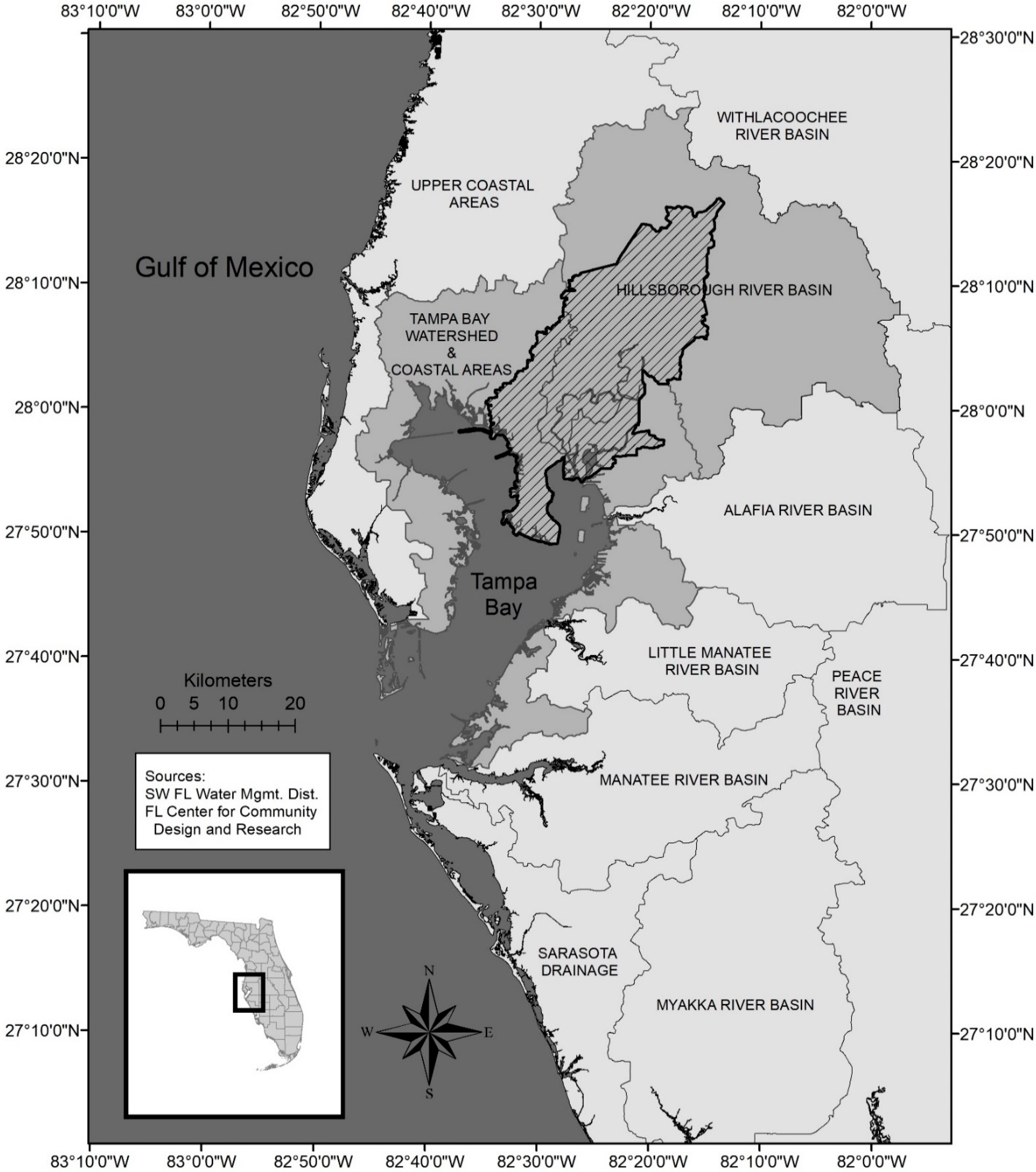
 Section 2.1 to Section 2.5 discusses the study area, data collection, and input datasets. 
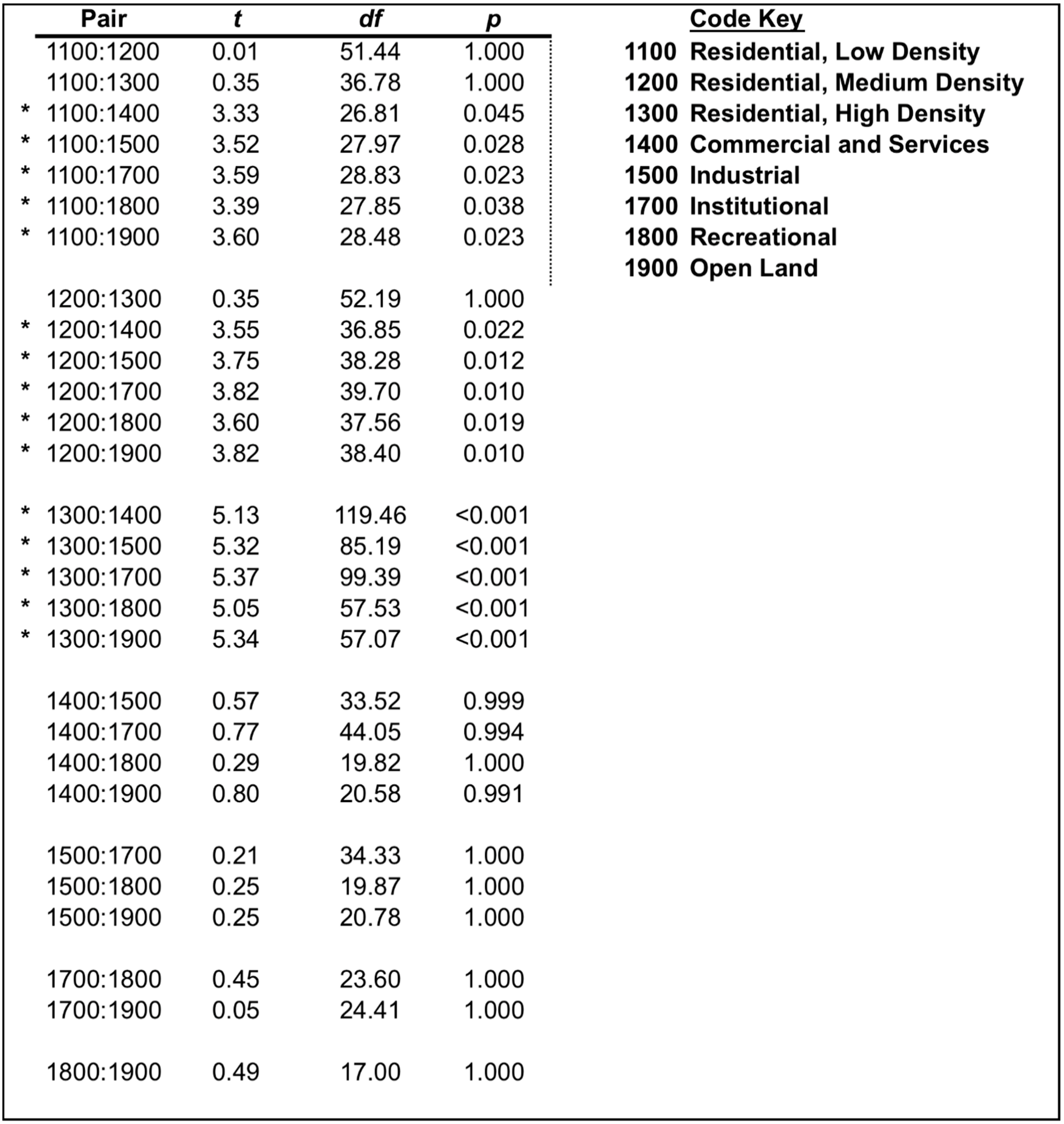
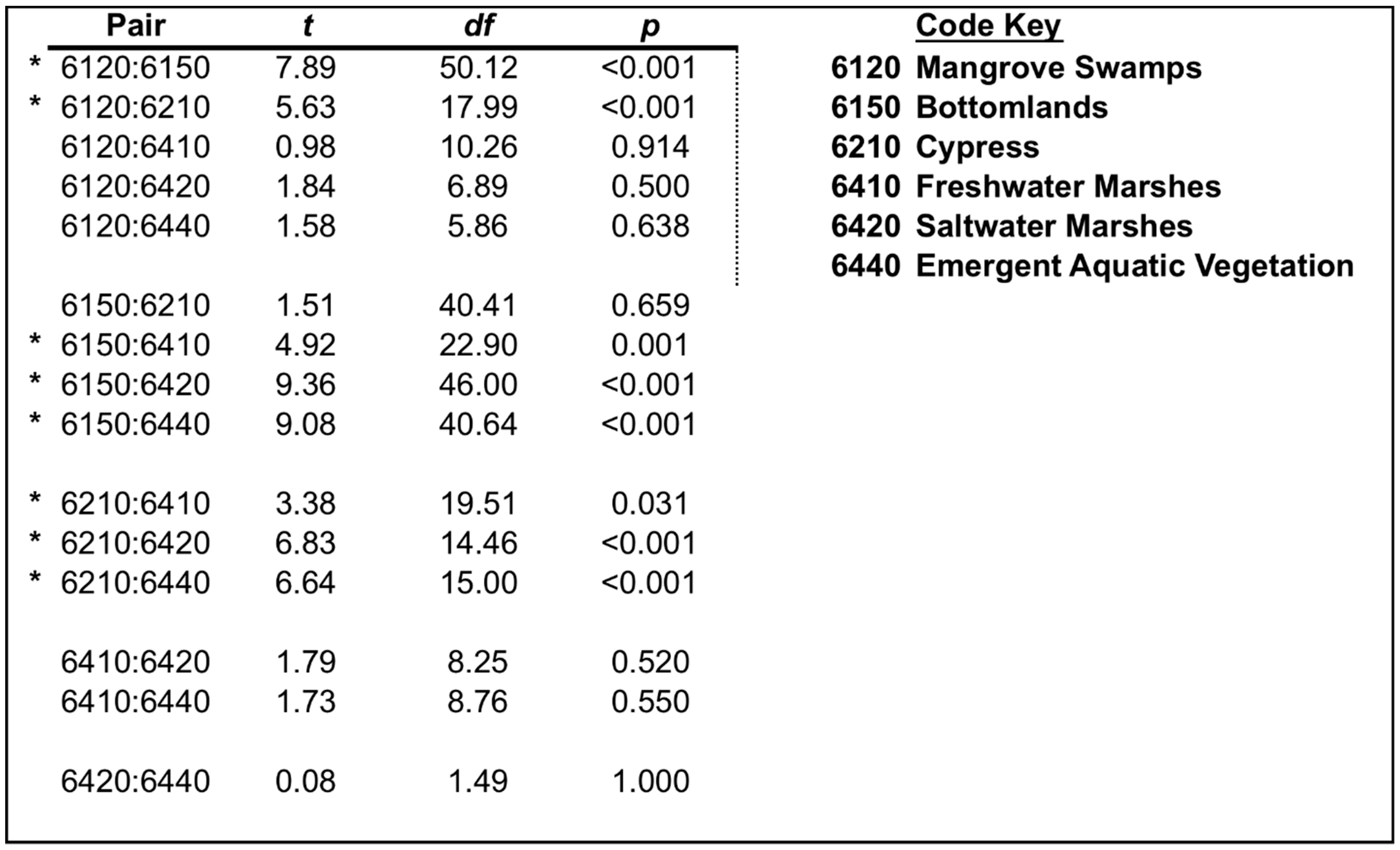
Section 2.6 discusses the statistical analyses to compare sub-classes for the plot data. Section 2.7 and Section 2.8 detail how the LULC classes were classified and then reclassified based on AGTC. Results for the initial classification and AGTC classification are detailed in Section 3.1 and Section 3.2, respectively. The post-hoc analyses to compare classes are discussed in Section 3.3. The structural classification using a decision tree is discussed in 
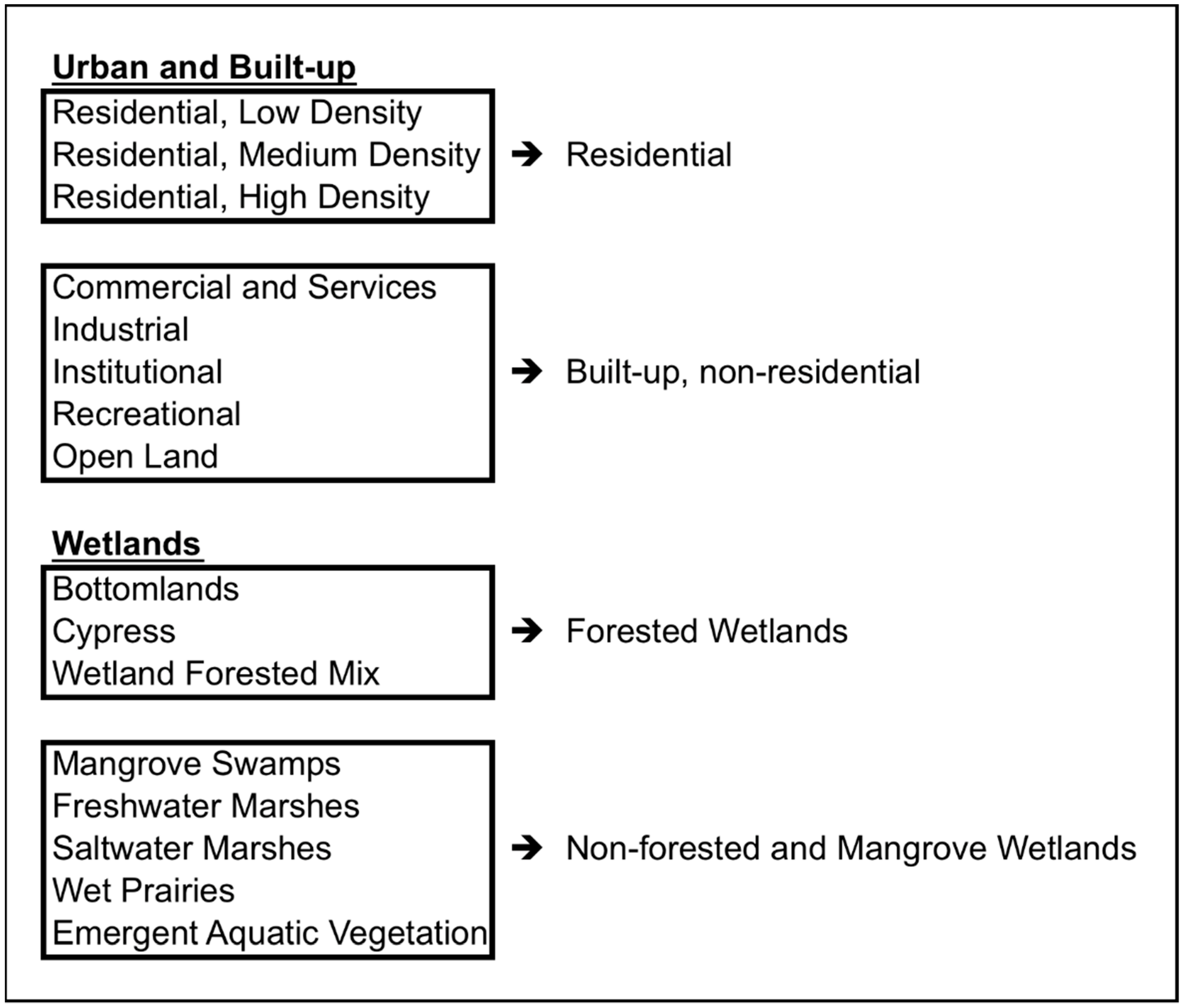
Section 3.4 while the final reclassification is detailed in Section 3.5.

2. Materials and Methods

2.1. Study Area

This study was conducted in a 796 km2 (79,600 ha) subbasin of the Tampa Bay Watershed (TBW) adjacent to the city of Tampa, Florida in the southeastern United States (27.95° N, 82.46° W) (Figure 1). The TBW is located in west-central Florida along the Gulf of Mexico. It spans 16,600 km2 with a drainage basin of 5700 km2 [42]. It is the largest estuary in the state with approximately 100 tributaries, 4 rivers, and 40 brackish streams. The TBW has a humid subtropical climate with a mean annual temperature of 23.3 °C. Winters are short, dry, and mild with roughly 1–2 freezes per year. Most rain occurs during summer months ranging from late April to October. Mean annual precipitation is 127 cm.
The area is home to approximately 4.6 million people in Hillsborough, Manatee, Pasco, and Pinellas counties. These include the cities of Tampa, St. Petersburg, and Clearwater. Florida itself has experienced rapid population growth in the past few decades with urban expansion occurring at a rate faster than the national average [43]. The TBW is no exception with the addition of 1,000,000 people during the period 1995–2005 [44].
As an important urban center of Florida, the TBW contains productive agricultural lands, phosphate mining, power generation, tourism, recreation, and other industries. These activities have led to significant environmental degradation and LULC change [45].

2.2. Plot Data

The study area was divided into a grid of 1.77 km2 hexagons with a random sample point selected in each as specified by the UFORE model framework [46]. A total of 531 plots (Figure 2), each 405 m2 were inventoried, using the procedures in the UFORE field data collection manual, including species and diameter at breast height (DBH) for all individual tree stems greater than or equal to 2.5 cm [47]. Percent cover, count, and species data were also recorded for all tree and non-tree woody stems less than 2.5 cm but were not included in this study due to difficulties obtaining carbon estimates. Plots were sampled in 2006 and resampled in 2011. Any plots that were not resampled were removed from analyses as discussed in Section 2.5. Species were identified to specific epithet when possible; otherwise down to genera using nomenclature established in the Plant List of Accepted Nomenclature, Taxonomy, and Symbols (PLANTS) database developed by the Natural Resources Conservation Service, an agency of the United States Department of Agriculture [48].

2.3. Carbon Estimates

AGTC estimates for individual trees were obtained using the UFORE model. Individual tree estimates were then summed to derive a total AGTC estimate for each sample plot. UFORE was developed by the US Forest Service to estimate structure, carbon storage, and air quality for cities [46]. UFORE has been used in a number of North American cities including New York, Washington DC, Baltimore, San Francisco, Toronto, and international cities in China, New Zealand, and Italy, among others [49,50,51]. It was later expanded into a larger suite of modeling tools known as i-Tree [52].

2.4. LULC Data and Initial Classification

Plot LULC classifications were obtained using data available from the Southwest Florida Water Management District (SWFWMD) [53]. SWFWMD LULC data cover an area much larger than the TBW available as 1:100,000 quarter quadrangles. Quadrangles for 2006 and 2011 were processed to derive LULC maps covering portions of Hillsborough and Pasco counties within the study area’s boundaries.
The SWFWMD datasets used a classification scheme derived specifically for Florida and adapted from the Florida Fish and Wildlife Conservation Commission’s (FWC) Florida Land Use Cover Classification System (FLUCCS) [54]. FLUCCS itself is based on a framework design [29] that breaks land use and land cover categories into a four-tier hierarchy [55]. Each tier increases in detail and specificity from Level I (coarse) to Level IV (detailed). For example, using SWFWMD’s adaptation of this system, the broad Level I category “Agriculture” is numbered “2000”. Any sub-class within "Agriculture" is a Level II class, numbered as 2X00. For the "Agriculture" class, this corresponded to four sub-classes numbered with the 2X00 convention: “Cropland and Pastureland” (2100), “Tree Crops” (2200), “Nurseries and Vineyards” (2400), and “Other Open Lands” (2600). The final two levels in the hierarchy, Level III and Level IV, are additional sub-classes of each preceding level. In many cases, classes go no further than Level II. Using this framework, the Florida Department of Transportation created a set of urban and built-up classifications for the entire state [55]. FWC adapted these to include classes representing vegetative communities occurring throughout the state [41]. SWFWMD refined these even further for use along the west-central Gulf Coast of Florida where it conducts its operations [54]. One benefit of using SWFWMD FLUCCS datasets is their consistency in application. FLUCCS is the standard classification system used by agencies of the State of Florida and readily understood by their personnel. Furthermore, it is based on the Anderson classification, itself a standard in LULC studies [29,30]. Finally, with 53 Level II and III classes within eight Level I umbrella classes, it provides one of the more detailed schematics allowing for greater control over its modification. The resultant LULC maps contained eight Level I categories (Table 1, Table 2 and Table 3).

2.5. Data QA/QC

LULC classifications were compared with ground-truth field observations during data collection. Classifications that were inconsistent were removed. In addition, a number of the plots sampled in 2006 were not resampled in 2011. Likewise, some plots were added in 2011 that were not originally sampled in 2006. Plots without data for both years were removed.
Finally, plots that experienced land-use or land-cover change between 2006 and 2011 were also removed. This was to ensure that changes in AGTC over time reflected processes within the class and not the act of LULC change itself. There were initially 531 plots, with 409 (approximately 77%) remaining after removing plots to account for the above constraints.

2.6. AGTC Classification

Level II FLUCCS classes within each Level I category were tested for differences in AGTC (kg plot−1). Each plot was taken as one sample point. A one-way analysis of variance AOV (α = 0.05) was used to compare sub-classes in each of the eight Level I categories. If AOV results showed no difference between all combinations of sub-classes, they remained together with the same Level I category and were considered a final LULC class.
The AOV test indicates whether differences exist between two or more sub-classes but does not specify which classes differ. Therefore, any Level I class that showed a significant difference between two or more sub-classes was investigated using a post-hoc analysis. The Games–Howell pairwise comparison was used to determine which sub-classes were significantly different. This test is appropriate for groups with unequal sample sizes and heterogeneous variances [56,57].

2.7. Structure Classification

The AGTC-based analysis grouped or split classes based on differences in carbon alone. It did not reveal any information about canopy structure or socio-economic influences within the classes. This information might be useful to understand the distribution of AGTC across the landscape. This analysis creates a classification based on these considerations with no inclusion of the SWFWMD land use and land cover classes. The RPART package in R was used to create a decision tree that partitioned plot data by analyzing a group of input variables [58]. Sample plots were partitioned into groups or “bins” to predict the dependent variable. In this case, the actual predictions of the dependent variable (AGTC) were not of interest. Instead, the split points, based on the input variables, were extracted from the tree and incorporated into the LULC classification described earlier.
Six plot-level independent variables were included in the tree to test for their predictive ability to partition the data: percent impervious surface, plot legacy, political boundary, stem count, zoning code, and basal area (m2 plot−1). Impervious surface, stem count, and basal area (BA) were calculated using information provided in the initial plot inventory. Plot legacy was a categorical variable that described the legacy of vegetation on the plot defined as remnant, emergent, or managed. A plot was designated remnant if it contained vegetation at least as early as 1948 up to 2007. Emergent plots held no vegetation in 1948 but were vegetated in 2007. Managed plots were those with current, actively managed vegetation. Political boundary was either “Tampa” or “Exterior”, referring to a plot’s location either within the City of Tampa proper, or outside of the city but within in the subbasin boundaries of greater Hillsborough and Pasco counties. Zoning codes were obtained from Hillsborough and Pasco Counties [59,60].
The algorithm used in the Recursive Partitioning and Regression Trees (RPART) package accomplished two tasks. First, it tested which variables were most significant in partitioning the data. It then used these variables to determine split points and a set of decision rules used to classify the plots. In effect, the final tree only used those variables determined to be best for partitioning the data, given user-defined settings on how deep to grow the tree. For a full description of RPART and the Classification and Regression Trees (CART) packages, see Therneau and Atkinson [61].

2.8. Coupled Reclassification

Results from the AGTC and structure classifications were merged to create the final classification. Splitting a class into two or more sub-classes created the opportunity to observe nuances in the data at the cost of greater complexity. Furthermore, an increase in classes reduced the sample size of each new sub-class. To retain statistical power, partitions were restricted in classes with a sample size less than twenty.

3. Results

3.1. Initial FLUCCS Classification

SWFWMD FLUCCS codes comprised 53 Level II to III classes across eight Level I categories [54]. Of these, plot data represented seven Level I categories and 33 Level II or III classes (Table 1, Table 2 and Table 3). With a total of 409 plots across 33 classes, many contained very few plots. In particular, “Golf Courses” (1820), “Mixed Rangeland” (3300), “Upland Coniferous Forest” (4100), “Wetland Forested Mix” (6300), and “Wet Prairies” (6430) had only one plot each. A further 13 classes had between 2 and 10 plots, 9 had between 11 and 30 plots, and 4 had greater than 30. The Level I “Urban and Built-up” class contained the majority of plots (276) across its 9 sub-classes. Of these sub-classes, the three residential classes (1100, 1200, and 1300) totaled 161 plots.

3.2. AGTC Classification

The AOV results (α = 0.05) indicated that sub-classes in four of the seven Level I categories were not significantly different (Table 4 and Table 5). These were “Agriculture” (p = 0.218), “Upland Forests” (p = 0.119), “Water” (p = 0.585), and “Transportation, Communication and Utilities” (p = 0.379). Since no significant differences were found, these sub-classes were merged and reclassified according to their Level I descriptions for the final classification.
The “Rangeland” class contained only two sub-classes: “Shrub and Brushland” and “Mixed Rangeland” (Table 1). Since “Mixed Rangeland” had only one plot, comparisons were not possible. Therefore, these sub-classes were merged to form the “Rangeland” class for the final classification.
Sub-classes within two Level I categories, “Urban and Built-up” and “Wetlands”, were significantly different (α = 0.05, p = 0.005 and p = 0.002 respectively). Post-hoc analyses were conducted to further investigate sub-class differences.

3.3. Post-Hoc Analyses

Pairwise comparisons were listed for the Level I “Urban and Built-up” and “Wetlands” classes (Figure 3 and Figure 4). To summarize, within the “Urban and Built-up” class, no differences were found between each of the three “Residential” classes (“High”, “Medium”, and “Low” housing densities). No significant differences were found between the other five urban sub-classes (“Commercial and Services”, “Industrial”, “Recreational”, “Institutional”, and “Open Land”). Significant differences were found between each of the “Residential” sub-classes and each of the other six urban classes. These results reveal two possible groups within the larger “Urban and Built-up” class: “Residential”, consisting of the three residential sub-classes; and an “Other urban” class, labeled as “Built-up, non-residential” (Figure 5).
Results for the “Wetlands” class reveal two possible groups based on the pairwise comparisons: a “Forested Wetlands” group consisting of the “Bottomlands” and “Cypress” sub-classes, and a “Non-forested & Mangrove Wetlands” group. This group was created from the “Freshwater Marshes”, “Saltwater Marshes”, “Emergent Aquatic Vegetation”, and “Mangrove Swamp” sub-classes because no significant differences were found between them. Finally, the “Wetland Forested Mix” sub-class (n = 1) was added to the new “Forested Wetlands” group, and the “Wet Prairies” sub-class (n = 1) was added to the “Non-forested Wetland” group (Table 6).

3.4. Structure Classification

The decision tree partitioned the plots into seven classes using BA and stem count (Figure 6). Impervious surface, political boundary, zoning codes, and site legacy were not included as partitioning variables based on importance tests for the six independent variables (Figure 7). Figure 7 lists the variables in terms of predictive importance from highest to lowest (top to bottom). The percent increase in mean square error (%IncMSE) measures the percent increase in misclassification, using mean square error (MSE) when a variable is randomly permuted. The MSE for a variable of low predictive importance changes slightly. Conversely, a greater percent change implies that a variable has greater importance in the model. In other words, it shows how much worse the model would perform without that variable [62]. The results, ranked from high to low importance, are as follows: BA (44.4%), stem count (16.32%), legacy (13.55%), zoning code (11.28%), impervious surface (7.49%), and political boundary (3.79%).
To reduce complexity and standardize the classes, tree depth was pruned one level to produce a final tree of five classes split on BA (Table 7, Figure 8). These split points determine how plots were placed into one of the five structure classes based on observed BA m2. The points were then incorporated into the LULC reclassification to derive the final classification described in the next section.

3.5. Final Classification

The final classes are based on the AGTC reclassification and BA/structure classification (Table 8). In total, there were fourteen final classes. The “Built, Non-residential”, “Residential”, and “Forested Wetlands” classes were further sub-divided using the structure classes. For others, the AGTC reclassification was kept intact and not further divided. This was performed with the objective of minimizing complexity and maximizing plots per class. For example, the “Rangeland” class had a total of six plots. Incorporating the structure classification was found to be infeasible, since it already had a very small number of plots. Similar decisions were made for the remainder of the classes. Additionally, the BA values shown in the final classification were scaled to BA ha−1.

4. Discussion

4.1. Comparison Examples

Regional studies often adopt classification systems developed by organizations interested in global or national-scale projects [63]. A few attempts have been performed to create comprehensive LULC classifications for the entire United States but often focus on more “natural” and resource related “covers”, neglecting the complexity of “uses” inherent in urban systems (e.g., National Resource Inventory, National Land Cover Dataset, and the United States Geological Survey Land Cover Trends Project) [63]. To overcome this, Theobald [63] constructed a national hierarchical classification scheme that focused on human landscape activities to better capture variation in outcomes from LULC change analyses. However, these efforts do not incorporate ecological data in the break-up of LULC classes and may potentially lose useful information in the variation in an ES across the landscape. This analysis modified an existing classification for use in a regional ES study. The reclassification incorporated variation in an ecosystem service (AGTC) between LULC classes. The intent was not to replace or standardize existing classifications, but rather to directly integrate ecological data into a classification scheme that includes both sociological and ecological LULC classes.
In their study of LULC change in suburban and urban regions in China, Ellis et al. [64] created a classification scheme that incorporated both land “forms” and land “uses”. According to their needs, the landforms component of the classification contained 27 classes, 16 of which were based on water flow features pursuant to the characteristics of the landscape and determined by visual interpretation of GPS data [64]. Variable data were directly incorporated into the classification scheme itself. Partitioning LULC classes using ES data provides a novel way to categorize the landscape for ES mapping studies. The results presented here can serve as a basis for future investigations into applicability and for comparisons using traditional classification schemes. In addition, the methodology can serve as a foundation for other regional studies to address a variety of ecosystem services.

4.2. Class Interpretations

Level I SWFWMD classes served as the foundation for the reclassification. This assumes these classes, which are based on both spectral and practical interpretations, are meaningful and/or accurate as a starting point in representing the landscape. For example, there is a degree of arbitrary interpretation in creating a “Residential” class as separate from a “Commercial” class in an urban setting. These interpretations are the basis for the “use” aspect of LULC classifications compared with land “cover” [65]. However, Level I classes were considered axiomatic for practical considerations, including ownership, access, and management that are real and valid in urban systems [66].
These considerations add to the complexity introduced when implementing Anderson Levels III and IV. Cadenasso et al. [31] introduced the concept of medium scale classification with their HERCULES model by including a percent cover of several factors in addition to the traditional interpretation of land use. For the structural classification, additional variables were tested to represent the forested “structure” of the landscape. The results showed that both stem count and basal area, two common forestry metrics, were better variables for partitioning the data relative to others included in the analysis. For example, the classification allows for the sub-division of “Residential” into “low”, “medium”, and “high” BA sub-classes, which adds more structural detail at the cost of greater complexity. For this reason, a mixed approach was taken when using the structural classification. Only including the structure split-points in the Level I categories that showed a significant difference in AGTC allowed for the use of BA in the scheme while limiting the complexity introduced. If the BA classes were applied to all Level I classes, the total split count would be three to four times higher, which is prohibitive with many LULC models.

4.3. Impervious Surface

An interesting result was the low ranking and exclusion of impervious surface from the decision tree. One possibility may be the distribution and size of landscape patches in Tampa. It would be useful to compare the patches of Tampa’s urban area with longer established cities with higher population densities and greater concentrations of built structures. It is possible that Tampa’s landscape may have more patch fragmentation between land use and land covers. As an urbanizing region, many of the suburban and exurban areas in the TBW contain patches of concrete and built structures interspersed with vegetation and water. However, cities with longer and more aggressive rates of development may be less fragmented with a more homogenous composition of impervious patches, though this was not investigated in the study. Additional fragmentation analyses can compare the TBW with other urban areas and may provide insights into differences of “urban-ness” between cities.

4.4. Structural Classification

The structural classification using BA was a useful approach to investigate novel enhancements of current classifications. In addition, the integration of the structural classification with the ES classification revealed inherent difficulties in added information. The combination of the structure and ES classifications resulted in 14 final classes. From an analysis standpoint, any increase in classes adds complexity. In addition, the determination of split-points within the integrated classes was objective at best. Lastly, it was difficult to apply the structure-based classification given available data for the entire TBW. While the ES classification can easily be applied to the landscape, due to available LULC maps provided by SWFWMD, similar spatial projections of BA for the entire TBW were not available. To apply the structure classification, each pixel of the landscape would need a BA value assessed from ground or remotely sensed data. It is possible that kriging or other interpolation methods can provide estimates, but a more complex investigation of structure-based classifications was beyond the scope of this study. However, it was noted that structure-based classifications are important for understanding ecosystem services. Therefore, methods to incorporate this information into existing classifications are a worthwhile endeavor and may become more applicable if future research provides BA estimates at the landscape scale.

4.5. Sample Sizes

Several LULC classes had relatively small sample sizes. However, the stratified sampling procedure ensured that, percentagewise, the number of plots for each class was representative of the percentage of total land for that class within the study area. Still, the result was a limitation on how Level I and II classes could be sub-divided to maximize statistical power. The trade-off between complexity and information was important. Although the structural classification introduced additional plot-level information, it would be imprudent to use this for every Level I class. If each class was further sub-divided, the final total would have been greater than 25 classes, with the majority having less than five plots each. Therefore, the BA partition was limited to the three classes with the highest number of plots, which in turn form the greatest percentage of the actual landscape (“Residential” = 32.64%, “Urban, non-residential” = 22.1%, and “Wetlands” = 14.99%).

5. Conclusions

This study created a novel LULC classification scheme by incorporating ecological data to redefine classes of the FLUCCS classification system based on variation in above-ground tree carbon. AOV and Games–Howell pairwise comparisons showed that sub-classes within a granted “land cover” class were similar for six of the seven classes. Significant differences were found within the “Wetlands” class based on vegetation cover, forming two distinct groups: “Forested Wetlands” and “Non-forested and Mangrove Wetlands”. The urban “land use” class showed differences between “Residential” and “Non-residential” sub-classes, forming two new classes respectively. This implies that LULC classifications can sometimes aggregate areas perceived as similar that are in fact distinct regarding ecological variables. These aggregations can obscure the true variation in a parameter at the landscape scale. Therefore, a study’s classification system should be designed to reflect landscape variation in the parameter(s) of interest.
The broad and interdisciplinary nature of this study also introduced several limitations which must be addressed. One is the relatively brief time span of tree data (2006–2011) from which AGTC change estimates were derived. In addition, tree and stand age were not collected, preventing a complete understanding of the relationship between growth and carbon quantities over time. Some of the LULC classes had relatively small sample sizes, impacting the statistical power of tests used in the analyses. The small sample sizes also introduced a degree of error as indicated by standard deviations which were higher than class means. This indicates that factors influencing landscape variation were not captured by the data. Future data collection efforts can provide additional time periods to incorporate into this analysis for a greater understanding of change over time.

Author Contributions

Conceptualization, J.J.L.IV, W.C.Z. and M.G.A.; data curation, J.J.L.IV; formal analysis, J.J.L.IV; funding acquisition, W.C.Z. and M.G.A.; methodology, J.J.L.IV; project administration, W.C.Z. and M.G.A.; resources W.C.Z. and M.G.A.; supervision W.C.Z. and M.G.A.; writing—original draft preparation, J.J.L.IV; writing—review and editing, J.J.L.IV, W.C.Z. and M.G.A. All authors have read and agreed to the published version of the manuscript.

Funding

This research was funded by a USDA Forest Service graduate research stipend. Additional supplemental funding provided by the following National Science Foundation grants: Urban Water Innovation Network (Award Number 1444758), Software Infrastructure for Transformative Urban Sustainability Research (Award Number 1931363), and the Urban Critical Zone UMBC Network Cluster (Award Number 2012340).

Institutional Review Board Statement

Not applicable.

Informed Consent Statement

Not applicable.

Data Availability Statement

The datasets generated and/or analyzed during the current study are available from the corresponding author on reasonable request.

Acknowledgments

We would like to thank Robert J. Northrop, Carolyn Cheatham Rhodes and Melissa Friedman for data collection efforts. Finally, we would like to thank Timothy A. Martin, Wendell P. Cropper, and Michael W. Binford for feedback on early drafts of the manuscript.

Conflicts of Interest

The authors declare no conflict of interest. The funders had no role in the design of the study; in the collection, analyses, or interpretation of data; in the writing of the manuscript, or in the decision to publish the results.

Abbreviations

%IncMSEPercent increase in mean square error
AGTCAbove-ground tree carbon
AOVAnalysis of variance
BABasal area
CARTClassification and Regression Trees
CO2Carbon dioxide
DBHDiameter at breast height
ESsEcosystem services
FLUCCSFlorida Land Use Cover Classification System
FWCFlorida Fish and Wildlife Conservation Commission
HERCULESHigh Ecological Resolution Classification for Urban Landscapes and Environmental Systems
LULCLand use and land cover
MSEMean square error
PLANTSPlant List of Accepted Nomenclature, Taxonomy, and Symbols
RPARTRecursive Partitioning and Regression Trees
SWFWMDSouthwest Florida Water Management District
TBWTampa Bay Watershed
UFOREUrban Forest Effects

References

  1. Alberti, M. Advances in Urban Ecology: Integrating Humans and Ecological Processes in Urban Ecosystems; Springer: New York, NY, USA, 2008. [Google Scholar]
  2. Schulp, C.J.; Nabuurs, G.J.; Verburg, P.H. Future carbon sequestration in Europe—Effects of land use change. Agric. Ecosyst. Environ. 2008, 127, 251–264. [Google Scholar] [CrossRef]
  3. Gitz, V.; Ciais, P. Future expansion of agriculture and pasture acts to amplify atmospheric CO2 levels in response to fossil-fuel and land-use change emissions. Clim. Chang. 2004, 67, 161–184. [Google Scholar] [CrossRef]
  4. Xian, G.; Crane, M. Assessments of urban growth in the Tampa Bay watershed using remote sensing data. Remote Sens. Environ. 2005, 97, 203–215. [Google Scholar] [CrossRef]
  5. Wu, J. Urban ecology and sustainability: The state-of-the-science and future directions. Landsc. Urban Plan. 2014, 125, 209–221. [Google Scholar] [CrossRef]
  6. Dwyer, J.F.; Nowak, D.J.; Heather Noble, M.; Sisinni, S.M. Connecting People with Ecosystems in the 21ST Century: An Assessment of Our Nation’s Urban Forests; General Technical Report PNW-GTR-490; USDA Forest Service, Pacific Northwest Research Station: Portland, OR, USA, 2000. [Google Scholar]
  7. United States Census Bureau. The 2010 United States Census. 2010. Available online: http://www.census.gov/2010census/ (accessed on 10 April 2019).
  8. Hooke, R.L.; Martín-Duque, J.F.; Pedraza, J. Land transformation by humans: A review. GSA Today 2012, 22, 4–10. [Google Scholar] [CrossRef]
  9. Elmqvist, T.; Setälä, H.; Handel, S.N.; Van Der Ploeg, S.; Aronson, J.; Blignaut, J.N.; Gomez-Baggethun, E.; Nowak, D.J.; Kronenberg, J.; De Groot, R. Benefits of restoring ecosystem services in urban areas. Curr. Opin. Environ. Sustain. 2015, 14, 101–108. [Google Scholar] [CrossRef] [Green Version]
  10. Goulder, L.H.; Kennedy, D. Interpreting and estimating the value of ecosystem services. In Natural Capital: Theory and Practice of Mapping Ecosystem Services; Oxford University Press: Oxford, UK, 2011; pp. 34–53. [Google Scholar]
  11. Bolund, P.; Hunhammar, S. Ecosystem services in urban areas. Ecol. Econ. 1999, 29, 293–301. [Google Scholar] [CrossRef]
  12. Sukopp, H.; Starfinger, U. Disturbance in urban ecosystems. In Ecosystems of the World; Peter Lang Publishing: New York, NY, USA, 1999; pp. 397–412. [Google Scholar]
  13. Gómez-Baggethun, E.; Barton, D.N. Classifying and valuing ecosystem services for urban planning. Ecol. Econ. 2013, 86, 235–245. [Google Scholar] [CrossRef]
  14. Jim, C.; Chen, W.Y. Ecosystem services and valuation of urban forests in China. Cities 2009, 26, 187–194. [Google Scholar] [CrossRef]
  15. Dobbs, C.; Escobedo, F.J.; Zipperer, W.C. A framework for developing urban forest ecosystem services and goods indicators. Landsc. Urban Plan. 2011, 99, 196–206. [Google Scholar] [CrossRef]
  16. Gómez-Baggethun, E.; Ruiz-Pérez, M. Economic valuation and the commodification of ecosystem services. Prog. Phys. Geogr. 2011, 35, 613–628. [Google Scholar] [CrossRef] [Green Version]
  17. Kosoy, N.; Corbera, E. Payments for ecosystem services as commodity fetishism. Ecol. Econ. 2010, 69, 1228–1236. [Google Scholar] [CrossRef]
  18. Daniel, T.C.; Muhar, A.; Arnberger, A.; Aznar, O.; Boyd, J.W.; Chan, K.M.; Costanza, R.; Elmqvist, T.; Flint, C.G.; Gobster, P.H.; et al. Contributions of cultural services to the ecosystem services agenda. Proc. Natl. Acad. Sci. USA 2012, 109, 8812–8819. [Google Scholar] [CrossRef] [Green Version]
  19. Bachelet, D.; Ferschweiler, K.; Sheehan, T.J.; Sleeter, B.M.; Zhu, Z. Projected carbon stocks in the conterminous USA with land use and variable fire regimes. Glob. Chang. Biol. 2015, 21, 4548–4560. [Google Scholar] [CrossRef]
  20. Jo, H.K.; McPherson, G.E. Carbon storage and flux in urban residential greenspace. J. Environ. Manag. 1995, 45, 109–133. [Google Scholar] [CrossRef] [Green Version]
  21. Nowak, D.J.; Crane, D.E. Carbon storage and sequestration by urban trees in the USA. Environ. Pollut. 2002, 116, 381–389. [Google Scholar] [CrossRef]
  22. Andreu, M.G.; Friedman, M.H.; Landry, S.M.; Northrop, R.J. City of Tampa Urban Ecological Analysis 2006–2007; Final Report to the City of Tampa; University of South Florida: Tampa, FL, USA, 2008; p. 24. [Google Scholar]
  23. Congalton, R.G. A review of assessing the accuracy of classifications of remotely sensed data. Remote Sens. Environ. 1991, 37, 35–46. [Google Scholar] [CrossRef]
  24. Crossman, N.D.; Burkhard, B.; Nedkov, S.; Willemen, L.; Petz, K.; Palomo, I.; Drakou, E.G.; Martín-Lopez, B. A blueprint for mapping and modelling ecosystem services. Ecosyst. Serv. 2013, 4, 4–14. [Google Scholar] [CrossRef]
  25. Burkhard, B.; Kroll, F.; Nedkov, S.; Müller, F. Mapping ecosystem service supply, demand and budgets. Ecol. Indic. 2012, 21, 17–29. [Google Scholar] [CrossRef]
  26. Commission of the European Communities. CORINE Land Cover; European Environment Agency: Brussels, Belgium, 1995. [Google Scholar]
  27. Burkhard, B.; Kroll, F.; Müller, F.; Windhorst, W. Landscapes’ capacities to provide ecosystem services—A concept for land-cover based assessments. Landsc. Online 2009, 15, 22. [Google Scholar] [CrossRef]
  28. Campbell, J.B.; Wynne, R.H. Introduction to Remote Sensing, 5th ed.; The Guilford Press: New York, NY, USA, 2011. [Google Scholar]
  29. Anderson, J.R. A Land Use and Land Cover Classification System for Use with Remote Sensor Data; US Government Printing Office: Washington, DC, USA, 1976; Volume 964. [Google Scholar]
  30. Jensen, J.R. Introductory Digital Image Processing: A Remote Sensing Perspective, 3rd ed.; Prentice Hall: Upper Saddle River, NJ, USA, 2005; p. 526. [Google Scholar]
  31. Cadenasso, M.L.; Pickett, S.T.; Schwarz, K. Spatial heterogeneity in urban ecosystems: Reconceptualizing land cover and a framework for classification. Front. Ecol. Environ. 2007, 5, 80–88. [Google Scholar] [CrossRef]
  32. Pickett, S.T.; Cadenasso, M.L. Linking ecological and built components of urban mosaics: An open cycle of ecological design. J. Ecol. 2008, 96, 8–12. [Google Scholar] [CrossRef]
  33. Pickett, S.T.; Burch, W.R.; Dalton, S.E.; Foresman, T.W.; Grove, J.M.; Rowntree, R. A conceptual framework for the study of human ecosystems in urban areas. Urban Ecosyst. 1997, 1, 185–199. [Google Scholar] [CrossRef]
  34. Cadenasso, M. Ecological heterogeneity in urban ecosystems: Reconceptualized land cover models as a bridge to urban design. In Resilience in Ecology and Urban Design; Springer: Dordrecht, The Netherlands, 2013; pp. 107–129. [Google Scholar]
  35. Zipperer, W.C.; Morse, W.; Gaither, C.J. Linking social and ecological systems. In Urban Ecology; Oxford University Press: Oxford, UK, 2011; pp. 298–308. [Google Scholar]
  36. Shi, Y.; Zhixin, Q.; Liu, X.; Niu, N.; Zhang, H. Urban land use and land cover classification using multisource remote sensing images and social media data. Remote Sens. 2019, 11, 2719. [Google Scholar] [CrossRef] [Green Version]
  37. Solórzano, J.V.; Mas, J.F.; Gao, Y.; Gallardo-Cruz, J. Land use land cover classification with U-Net: Advantages of combining Sentinel-1 and Sentinel-2 imagery. Remote Sens. 2021, 13, 3600. [Google Scholar] [CrossRef]
  38. Naushad, R.; Kaur, T.; Ghaderpour, E. Deep transfer learning for land use and land cover classification: A comparative study. Sensors 2021, 21, 8083. [Google Scholar] [CrossRef]
  39. Morgan Grove, J.; Cadenasso, M.L.; Burch, W.R., Jr.; Pickett, S.T.; Schwarz, K.; O’Neil-Dunne, J.; Wilson, M.; Troy, A.; Boone, C. Data and methods comparing social structure and vegetation structure of urban neighborhoods in Baltimore, Maryland. Soc. Nat. Resour. 2006, 19, 117–136. [Google Scholar] [CrossRef]
  40. Wu, J.J. Landscape ecology. In Ecological Systems; Springer: New York, NY, USA, 2013; pp. 179–200. [Google Scholar]
  41. Kawula, R. Florida Land Cover Classification System; Florida Fish and Wildlife Conservation Commission: Tallahassee, FL, USA, 2014. [Google Scholar]
  42. Seaber, P.; Kapinos, F.; Knapp, G. Hydrologic Unit Maps. In US Geological Survey, Water Supply Paper 2294; US Dept of the Interior: United States Government Printing Office: Washington, DC, USA, 1994. [Google Scholar]
  43. Tampa Bay Partnership. Tampa Bay’s Population Growth Surpasses Growth Rate of the Entire Nation. 2013. Available online: http://www.tampabay.org/about-us/news-media/partnership-blog/2013-08-15/tampa-bays-population-growth-surpasses-growth-rate (accessed on 12 March 2020).
  44. Florida Department of Environmental Protection. Learn about Your Watershed: Tampa Bay Watershed. 2015. Available online: http://www.protectingourwater.org/watersheds/map/tampa_bay/ (accessed on 12 March 2020).
  45. Xian, G.; Crane, M.; Su, J. An analysis of urban development and its environmental impact on the Tampa Bay watershed. J. Environ. Manag. 2007, 85, 965–976. [Google Scholar] [CrossRef]
  46. Nowak, D.J.; Crane, D.E. The Urban Forest Effects (UFORE) Model: Quantifying Urban Forest Structure and Functions; Gen. Tech. Rep. NC-212; U.S. Deptartment of Agriculture, Forest Service, North Central Forest Experiment Station: St. Paul, MN, USA, 2000. [Google Scholar]
  47. Nowak, D.J.; Crane, D.E.; Stevens, J.C.; Hoehn, R.E. The Urban Forest Effects (UFORE) Model: Field Data Collection Manual; USDA Forest Service: Portland, OR, USA, 2005. [Google Scholar]
  48. USDA-NRCS. The PLANTS Database; National Plant Data Team: Greensboro, NC, USA, 2015; p. 27491. [Google Scholar]
  49. Nowak, D.J.; Hoehn, R.E., III; Crane, D.E.; Stevens, J.C.; Walton, J.T. Walton Assessing Urban Forest Effects and Values, Washington, DC’s Urban Forest; USDA Forest Service: Newton Square, PA, USA, 2006. [Google Scholar]
  50. Nowak, D.J.; Hoehn, R.E., III; Crane, D.E.; Stevens, J.C.; Walton, J.T. Assessing Urban Forest Effects and Values, New York City’s Urban Forest; USDA Forest Service: Newton Square, PA, USA, 2007. [Google Scholar]
  51. Russo, A.; Escobedo, F.J.; Timilsina, N.; Schmitt, A.O.; Varela, S.; Zerbe, S. Assessing urban tree carbon storage and sequestration in Bolzano, Italy. Int. J. Biodivers. Sci. Ecosyst. Serv. Manag. 2014, 10, 54–70. [Google Scholar] [CrossRef]
  52. USDA Forest Service. i-Tree Eco User’s Manual, v5.0; USDA Forest Service: Portland, OR, USA, 2014. [Google Scholar]
  53. Southwest Florida Water Management District. Land-Use/Land Cover Maps SWFWMD Cover. Area (1995, 1999, 2004–2011); S.F.W.M. District: Brooksville, FL, USA, 2015. [Google Scholar]
  54. Southwest Florida Water Management District. Photo Interpretation Key for Land Use Classification; S.F.W.M. District: Brooksville, FL, USA, 2010; p. 173. [Google Scholar]
  55. Florida Department of Transportation. Florida Land Use Cover and Forms Classification System; Surveying and Mapping Office: Tallahassee, FL, USA, 1999. [Google Scholar]
  56. Games, P.A.; Howell, J.F. Pairwise multiple comparison procedures with unequal n’s and/or variances: A Monte Carlo study. J. Educ. Behav. Stat. 1976, 1, 113–125. [Google Scholar]
  57. Howell, D. Statistical Methods for Psychology; Cengage Learning: Belmont, CA, USA, 2012. [Google Scholar]
  58. R Core Team. R: A Language and Environment for Statistical Computing; R Foundation for Statistical Computing: Vienna, Austria, 2015. [Google Scholar]
  59. City of Tampa. City of Tampa Zoning Maps; City of Tampa: Tampa, FL, USA, 2015. [Google Scholar]
  60. Pasco County. Zoning Map; P.C. Department of Zoning and Intake: New Port Richey, FL, USA, 2015. [Google Scholar]
  61. Therneau, T.M.; Atkinson, E.J. An Introduction to Recursive Partitioning Using the RPART Routines; Mayo Foundation: Rochester, NY, USA, 2015. [Google Scholar]
  62. Breiman, L. Random forests. Mach. Learn. 2001, 45, 5–32. [Google Scholar] [CrossRef] [Green Version]
  63. Theobald, D.M. Development and applications of a comprehensive land use classification and map for the US. PLoS ONE 2014, 9, e94628. [Google Scholar] [CrossRef] [PubMed] [Green Version]
  64. Ellis, E.C.; Wang, H.; Xiao, H.S.; Peng, K.; Liu, X.P.; Li, S.C.; Ouyang, H.; Cheng, X.; Yang, L.Z. Measuring long-term ecological changes in densely populated landscapes using current and historical high resolution imagery. Remote Sens. Environ. 2006, 100, 457–473. [Google Scholar] [CrossRef]
  65. Comber, A.J. The separation of land cover from land use using data primitives. J. Land Use Sci. 2008, 3, 215–229. [Google Scholar] [CrossRef] [Green Version]
  66. Grove, J.M. Cities: Managing densely settled social-ecological systems. In Principles of Ecosystem Stewardship; Chapin, F.S., Kofinas, G.P., Folke, C., Eds.; Springer: New York, NY, USA, 2009; pp. 281–294. [Google Scholar]
Figure 1. The Tampa Bay Watershed in west-central Florida according to the Southwest Florida Water Management District. The hatched region shows the study area within the larger watershed.
Forests 13 00745 g001
Figure 2. The study area subbasin located inside the greater Tampa Bay Watershed showing sample plot locations within and around the City of Tampa, Florida.
Forests 13 00745 g002
Figure 3. Games–Howell pairwise comparisons of AGTC kg plot−1 between sub-classes of the “Urban and Built-up” Level I SWFWMD class. Significantly different sub-classes (at α = 0.05) are denoted with an asterisk.
Forests 13 00745 g003
Figure 4. Games–Howell pairwise comparisons of AGTC kg plot−1 between sub-classes of the “Wetlands” Level I SWFWMD class. Significantly different sub-classes (at α = 0.05) are denoted with an asterisk.
Forests 13 00745 g004
Figure 5. Group decisions based on AGTC kg plot−1 pairwise comparisons for Level II sub-classes of the Level I “Urban and Built-up” and “Wetlands” SWFWMD classes.
Forests 13 00745 g005
Figure 6. Unpruned RPART decision tree showing final bins and decision splits based on BA m2 plot. The top number in each box shows the mean AGTC kg for the n plots in that box. The percentage reflects each box’s plots as a proportion of the total number of plots (409).
Forests 13 00745 g006
Figure 7. Variable importance for the six variables used in the initial tree. The graphs show that BA is significantly more important for partitioning data on AGTC than the other five variables, followed by stem count.
Forests 13 00745 g007
Figure 8. Pruned RPART decision tree with final bins and decision splits based on BA m2 plot−1. The top number in each box shows the mean AGTC kg for the n plots in that box. The percentage reflects the number of plots in each box.
Forests 13 00745 g008
Table 1. Initial SWFWMD Level II FLUCCS sub-classes for the “Urban and Built-up”, “Agriculture”, and “Rangeland” Level I classes.
1000—Urban and Built-Up2000—Agriculture3000—Rangeland
1100Residential, Low Density, <2 Dwellings/Acre2100Cropland/Pastureland3200Shrub/Brushland
1200Residential, Med Density, 2–5 Dwellings/Acre2200Tree Crops3300Mixed Rangeland
1300Residential, High Density, >5 Dwellings/Acre2400Nurseries and Vineyards
1400Commercial and Services2600Other Open Lands—Rural
1500Industrial
1700Institutional
1800Recreational
1820Golf Courses
1900Open Land
Table 2. Initial SWFWMD Level II FLUCCS sub-classes for the “Upland Forests” and “Water” Level I classes.
4000—Upland Forests5000—Water
4100Upland Coniferous Forest5100Streams and Waterways
4110Pine Flatwoods5200Lakes
4340Upland Hardwood/Coniferous Mix5300Reservoirs
4400Tree Plantation5400Bays and Estuaries
Table 3. Initial SWFWMD Level II FLUCCS sub-classes for the “Wetlands” and “Transportation, Communication, and Utilities” classes.
6000—Wetlands8000—Transportation, Communication, Utilities
6120Mangrove Swamps8100Transportation
6150Bottomlands8300Utilities
6210Cypress
6300Wetland Forested Mix
6410Freshwater Marshes
6420Saltwater Marshes
6430Wet Prairies
6440Emergent Aquatic Vegetation
Table 4. AOV results to test for differences in plot AGTC (kg) between sub-classes for Level I “Urban and Built-up”, “Agriculture”, and “Upland Forest” classes (p: p-value; F: F-value; df: degrees of freedom).
1000—Urban and Built-Up2000—Agriculture4000—Upland Forests
pFdfpFdfpFdf
0.005 a3.0070.2181.7310.1192.771
a Level I classes with significantly different sub-classes (α = 0.05).
Table 5. AOV results to test for differences in plot AGTC (kg) between sub-classes for Level I “Water”, “Wetlands”, and “Transportation, Communication, and Utility” classes (p: p-value; F: F-value; df: degrees of freedom).
5000—Water6000—Wetlands8000—Trans., Comm., and Utilities
pFdfpFdfpFdf
0.5850.6730.002 a4.0850.3790.81
a Level I classes with significantly different sub-classes (α = 0.05).
Table 6. Class equivalencies between original SWFWMD classes and new land use/land cover classes after applying AOV and post-hoc analyses.
Reclass ResultsFLUCCS Classes Used
ResidentialResidential, Low Density; Residential, Med Density; Residential, High Density
Built-up,
Non-residential
Commercial and Services; Industrial; Institutional; Recreational; Golf Courses; Open Lands
AgricultureCropland and Pastureland; Tree Crops; Nurseries and Vineyards; Other Open Lands, Rural
RangelandShrub and Brushland; Mixed Rangeland
Upland ForestsUpland Coniferous Forests; Pine Flatwoods; Upland Hardwood/Coniferous Mix; Tree Plantation
WaterStreams and Waterways; Lakes, Reservoirs; Bays and Estuaries
Forested WetlandsBottomlands; Cypress; Wetland Forested Mix
Non-forested and Mangrove WetlandsMangrove Swamps; Freshwater Marshes; Saltwater Marshes; Wet Prairies; Emergent Aquatic Vegetation
InfrastructureTransportation; Utilities
Table 7. Split points used to partition plot data into five structure classes based on BA (m2 plot−1).
Class #Split Point
1<0.31
20.31 to 0.68
30.68 to 1.19
41.20 to 2.50
5>2.50
Table 8. Final classification combining AGTC classification with BA classification. BA values are shown scaled (m2 ha−1).
ClassNumber of Plots
Agriculture12
Built, Non-residential, BA < 882
Built, Non-residential, BA 8 to 6222
Forested Wetlands, BA 0 to 2919
Forested Wetlands, BA 29.1 to 6234
Forested Wetlands, BA > 6210
Infrastructure28
Non-Forested and Mangrove Wetlands21
Rangeland6
Residential, BA < 873
Residential, BA 8 to 1742
Residential, BA 17.1 to 6226
Upland Forests17
Water17
Publisher’s Note: MDPI stays neutral with regard to jurisdictional claims in published maps and institutional affiliations.

