Article

Configuration of the Deep Neural Network Hyperparameters for the Hypsometric Modeling of the Guazuma crinita Mart. in the Peruvian Amazon

by
Gianmarco Goycochea Casas
1,*,
Duberlí Geomar Elera Gonzáles
2,
Juan Rodrigo Baselly Villanueva
3,
Leonardo Pereira Fardin
1 and
Hélio Garcia Leite
1
1
Department of Forest Engineering, Federal University of Viçosa, Viçosa 36570-900, MG, Brazil
2
Departamento de Ciencias Forestales, Escuela de Ingeniería Forestal y Ambiental, Universidad Nacional Autónoma de Chota, Jr. José Osores Nro. 418, Chota, Cajamarca 06121, Peru
3
Baños del Inca Agrarian Experimental Station, National Institute of Agrarian Innovation, Jr. Wiracocha s/n, Baños del Inca, Cajamarca 06004, Peru
*
Author to whom correspondence should be addressed.
Forests 2022, 13(5), 697; https://doi.org/10.3390/f13050697
Submission received: 30 March 2022 / Revised: 18 April 2022 / Accepted: 21 April 2022 / Published: 29 April 2022
(This article belongs to the Special Issue Modeling of Forest Tree and Stand Parameters)

Abstract

:
The Guazuma crinita Mart. is a dominant species of great economic importance for the inhabitants of the Peruvian Amazon, standing out for its rapid growth and being harvested at an early age. Understanding its vertical growth is a challenge that researchers have continued to study using different hypsometric modeling techniques. Currently, machine learning techniques, especially artificial neural networks, have revolutionized modeling for forest management, obtaining more accurate predictions; it is because we understand that it is of the utmost importance to adapt, evaluate and apply these methods in this species for large areas. The objective of this study was to build and evaluate the efficiency of the use of a deep neural network for the prediction of the total height of Guazuma crinita Mart. from a large-scale continuous forest inventory. To do this, we explore different configurations of the hidden layer hyperparameters and define the variables according to the function HT = f(x) where HT is the total height as the output variable and x is the input variable(s). Under this criterion, we established three HT relationships: based on the diameter at breast height (DBH), (i) HT = f(DBH); based on DBH and Age, (ii) HT = f(DBH, Age) and based on DBH, Age and Agroclimatic variables, (iii) HT = f(DBH, Age, Agroclimatology), respectively. In total, 24 different configuration models were established for each function, concluding that the deep artificial neural network technique presents a satisfactory performance for the predictions of the total height of Guazuma crinita Mart. for modeling large areas, being the function based on DBH, Age and agroclimatic variables, with a performance validation of RMSE = 0.70, MAE = 0.50, bias% = −0.09 and VAR = 0.49, showed better accuracy than the others.

1. Introduction

The Guazuma crinita Mart. (Bolaina Blanca) is characterized as a fast-growing forest species established in plantations in which it reaches growth maturity by the eighth or ninth year, being ready for harvesting [1,2]. The wood has a high commercial value and is used to obtain round and sawn wood for the manufacture of stretchers, boxes, laminates, toys, matches, handicrafts, plywood, construction and coating of houses and the obtaining of cellulose for paper, contributing to the livelihood of local farmers [3,4]. According to the Servicio Nacional Forestal y de Fauna Silvestre [5], there is 8530.76 ha of Bolaina Blanca plantations in Peru, which represents 503,839.71 m3 of standing trees.
A hypsometric model is generally expressed between the height and diameter relationship of a tree; however, it has also been shown that the variables of age, basal area, site index, number of individuals per hectare, quadratic diameter, diameter and age classification, have influence with height [6,7]. It is very common to apply hypsometric modeling to reduce the costs and time of an inventory, as well as to contribute to the planning and forecasting of the volumetric production of plantations [8,9].
Deep learning is a type of automatic learning in which the same pattern of an artificial neural network (ANN) is followed, i.e., an architecture is defined and connections between them are shown [10]. ANNs often work with a single hidden quantity layer, but when used larger they are called deep neural networks (DNNs) or deep learning [11]. In other words, the big difference between ANN and DNN is that the latter model allows for multiple computations using processing layers to learn data representations with various levels of abstraction [11,12].
Hyperparameters are defined as parameters whose values control the learning process. A hyperparameter exploration is performed in order to test various configurations to obtain a better-performing model. This process is called hyperparameter optimization [13]. Such optimization can be done manually using empirical rules [14] or also with automated search [15], to reduce processing time and human effort, increasing productivity and throughput in scientific studies [16].
DNNs have been used to solve complex problems in the forestry and environmental area, such as identification of the origin of carbon through macroscopic images [17], to map Amazonian palm species at the individual tree crown level (ITC) using images RGB [18], species classification based on terrestrial laser scanning [19], for a rapid and efficient evaluation of forest damage after an environmental disaster [20]. It has even been shown in various studies related to forest management that the use of machine learning techniques is more accurate than mathematical regression techniques in their statistical performance [21,22,23,24,25,26,27,28].
The use of deep learning has not found studies for hypsometric modeling of this species, either in the Peruvian Amazon territory, this being the main problem when a base of its adequate configuration is not found to model the height. We consider it extremely important to understand the development of the DNN with hypsometric modeling, especially when large areas and a large amount of data from the continuous forest inventory of Bolaina Blanca are housed. Our hypothesis was that the configuration of the hyperparameters directly affects the statistical estimates in the hypsometric modeling of the Bolaina Blanca. The objective of this study was to evaluate the efficiency of using a deep learning neural network to predict the total height of Guazuma crinita Mart. from a large-scale continuous forest inventory, having specific objectives: (i) to configure and train the neural network and (ii) to evaluate the performance of the functions for total height prediction.

2. Material and Method

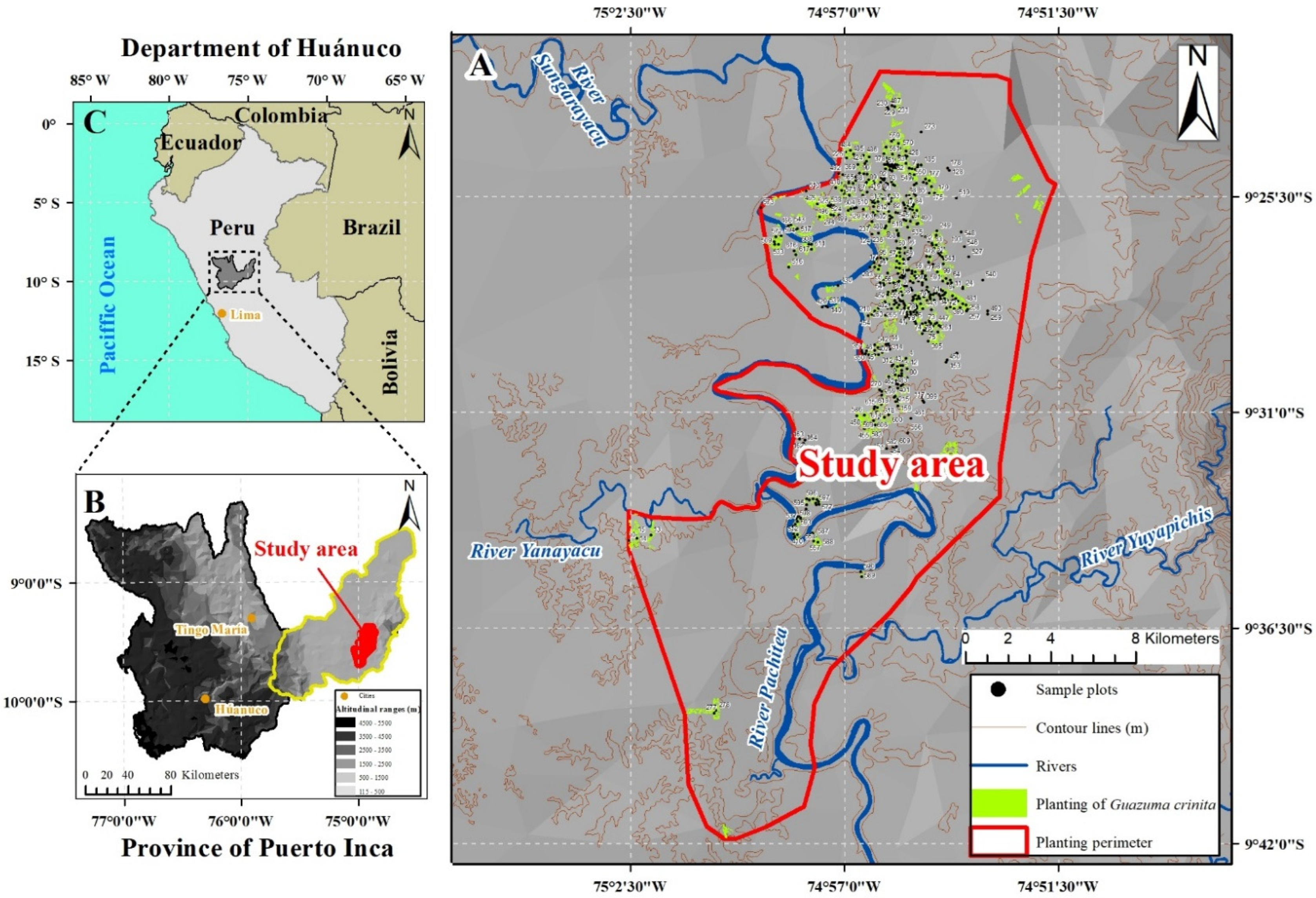
2.1. Study Area and Database

The Guazuma crinita Mart. forest plantations are located between parallels 9°22′0.32′′ and 9°41′52.60′′ S and meridians 74°51′03.18′′ and 75°02′33.18′′ W, between the districts of Puerto Inca and Yuyapichis, province of Puerto Inca, department of Huánuco, in the central Amazonian of Peru (Figure 1). The database comes from continuous forest inventory plots with measurements taken in the period 2009 to 2016. Data from 626 permanent measurement plots (PPM) were used, rectangular in shape randomly distributed with dimensions from 403 to 1509 m2, with a total of 135,016 measurements equivalent to an area of 9834 hectares, with plot information: number, area, age, number of trees per plot, diameter at breast height measured at 1.3 m height (DBH) and total height (HT), measured with caliper and suunto hypsometer, respectively. Table 1 shows their descriptive statistics of dendrometric and agroclimatological variables.
The plantations are distributed at altitudes that vary between 180 and 500 m above sea level, the average annual temperature is 27 °C, the average annual relative humidity is 85% and the annual precipitation varies between 2000 and 3000 mm, with greater intensity of precipitation between the months of November to March [29]. According to Holdridge [30] life zone classification, the study area is located in a region covered by tropical humid forest (bh-T), very humid tropical forest (bmh-T), and very humid transitional tropical forest (bmh-TT).
In this study we used agroclimatic variables extracted from the NASA Prediction Of Worldwide Energy Resources website: https://power.larc.nasa.gov/ (accessed on 12 November 2021). Through the coordinates of each plot from 2009 to 2016, using the annual average in the predictions. The downloaded variables were: Surface Pressure (kPa), Temperature at 2 Meters (°C), Specific Humidity at 2 Meters (g/kg), Relative Humidity at 2 Meters (%), Wind Speed at 2 Meters (m/s), Surface Soil Wetness, Temperature at 2 Meters Maximum (°C), Temperature at 2 Meters Minimum (°C), Profile Soil Moisture, Root Zone Soil Wetness, Wind Speed at 2 Meters Maximum (m/s), Wind Speed at 10 Meters Maximum (m/s), Wind Speed at 10 Meters Minimum (m/s), Precipitation Corrected (mm/day), Wind Speed at 10 Meters Range (m/s), All Sky Surface UVA Irradiance (W/m2), All Sky Surface UVB Irradiance (W/m2), All Sky Surface Shortwave Downward Irradiance (MJ/m2/day), Clear Sky Surface Shortwave Downward Irradiance (MJ/m2/day), All Sky Surface PAR Total (W/m2) and Clear Sky Surface PAR Total (W/m2).

2.2. Variable Input, Output, and Data Splitting in Training and Validation

For model fitting, we used the technique of deep artificial neural networks using the H20 pack [31] in R [32]. We set the function HT = f(x), where HT is the output variable and x is the input variable(s). Under this criterion, we established three HT relationships: depending on the DBH variable, (i) HT = f(DBH); based on DBH and Age, (ii) HT = f(DBH, Age) and based on DBH, Age and agroclimatic variables, (iii) HT = f(DBH, Age, Agroclimatology), respectively. All downloaded agroclimatic variables were included in the third function. These functions were trained separately, they were configured with different hyperparameters and their performance was compared. In total, we performed 72 training runs, i.e., 24 training models for each HT = f(x) function set in this study.
The data was standardized and randomly separated establishing 70% of the data for Training and 30% for Validation.

2.3. Hyper-Parameter Tuning

2.3.1. Layers, Units, and Activation Function

Their architectures had one input layer, two, three, and five hidden layers and one output layer. The numbers of neurons or units in the hidden layer were 10:10 (Figure 2A), 10:5 (Figure 2B), 10:5:2 (Figure 2C), 50:50 (Figure 2D), 50:25 (Figure 2E), 50:25:5 (Figure 2F), 10: 5:2:5:10 (Figure 2G), and 50:25:5:25:50 (Figure 2H).
The Tanh (Equation (1)), Rectified Linear (Equation (2)), and Maxout (Equation (3)) activation functions were used in the hidden layer, while in the output layer we use the Linear (Equation (4)) activation function for all cases.
f ( α ) = e α e α e α + e α ; f ( . ) [ 1 , 1 ]
f ( α ) = max ( 0 , α ) ; f ( . ) +
f ( . ) = max ( w i x i + b ) ; f ( . ) [ , 1 ] ;   rescale   if   max   f ( . )     1  
f ( α ) = α  
where f is the function that represents the non-linear activation used in the entire neural network, b is the bias for the neuron activation threshold, xi and wi denote the input values of the unit or neuron and their weights; α denotes the weighted combination:
α = j = 1 n w i x i + b .  

2.3.2. Distribution and Loss Functions

The Gaussian distribution function was specified as equivalent to wMSE (weighted mean squared error) (Equation (5)) as it was, our numerical response variable and the loss function chosen was quadratic (Equation (6)):
f ( . ) = ω ( y f ) 2
where y is a true response, f is a predicted response, and ω is weighted.
L ( W , B | j ) = 1 2 | t ( j ) o ( j ) 2 2
where t ( j ) and o ( j ) are the predicted and actual output; j and W is the collection { W i } 1 : N 1 : W i denotes the weight matrix connecting layers i and i + 1 for a network of N layers; B is the collection { b i } 1 : N 1 : b i denotes the column vector of biases for layer i + 1.

2.3.3. Optimization Algorithm, Regularization, Epoch, and Batch Size

The optimization algorithm used in this study was the adaptive learning rate ADADELTA (Equation (7)) [33]. The mini-batch was of size 1, the number of epochs was 300, and the type of regularization was with the early stop system, with 5 stop rounds, stop tolerance of 0.001, and MSE (mean square error) stop metric.
E [ g 2 ] t = ρ E [ g 2 ] t 1 + ( 1 ρ ) g t 2 ;   Accumulate   Gradient Δ θ t = R M S [ Δ θ ] t 1 R M S [ g ] t g t ;   Compute   Update E [ Δ θ 2 ] t = ρ E [ Δ θ 2 ] t 1 + ( 1 ρ ) Δ θ t 2 ;   Accumulate   Updates θ t + 1 = θ t + Δ θ t ;   Apply   Update }
where θ t denoting the parameters at the t-th iteration, g t is the compute gradient, t is the time and RMS is the root mean squared error. For our study, the learning rate time decay factor (rho) was 0.99 and the learning rate time smoothing factor (epsilon) was 1 × 10⁻⁸.

2.4. Model Performance

The estimates were analyzed according to [8,34]. The estimates of the training and testing data were with the statistical variables of Root Mean Squared Error, RMSE (Equation (8)), and Mean Absolute Error, MAE (Equation (9)). For testing data, we increased bias% (Equation (10)) and the variance error, VAR (Equation (11)). Likewise, percentage graphs of cases by percentage relative error, RE% (Equation (12)) were also interpreted. Figure 3 shows the methodological flowchart used in this study.
R M S E = n 1 i = 1 n ( Y i Y i ^ ) 2
M A E = ( n 1 i = 1 n | Y i Y i ^ | )
B i a s % = B i a s Y ¯ × 100 ;   B i a s = i = 1 n Y i Y i ^ n
V A R = ( b i a s ( Y i Y i ^ ) ) 2 n 1  
R E % = Y i Y i ^ Y × 100
where n = the number of observations for the measurer, Y i = observed total height valuei, Y i ^ = predicted total height valuei, and Y ¯ = mean of observed total height valuei.
The data were processed with the following computer features:
-
Operating System: Windows 10 Pro 64-bit
-
CPU: Intel Core i3 6006U @ 2.00 GHz- Skylake-U/Y 14 nm Technology
-
RAM: 12.00 GB Dual-Channel Unknown @ 1064MHz (15-15-15-35)
-
Motherboard: LENOVO LNVNB161216 (U3E1)
-
Graphics: Generic PnP Monitor (1366 × 768@64 Hz)
-
Storage: 465 GB Western Digital WDC WDS500G2B0B-00YS70 (SATA (SSD).

3. Results

3.1. Training Status

The maximum processing time for each model was 50 s. In Table 2 we can observe the status and architecture of each trained model according to each function. The trained models it was not necessary to complete the complete training epochs (300 epoch).
The networks trained from the HT = f(DBH) function obtained between 5.4 and 195.7 training epochs, 509,363 and 1,8497,950 training samples, 91 and 6061 weights and bias. The HT = f(DBH, Age) function was obtained between 6.7 and 158.9 training epochs, 637,904 and 15,100,404 training samples, 101 and 6161 weights and biases. The HT = f(DBH, Age, Agroclimatology) function was obtained between 5.7 and 44.4 training times, 542,308 and 4,197,664 training samples, 311 and 8261 weights and biases.
Complete training status of each model and type of function evaluated used to predict the total height of Guazuma crinita Mart. in the Peruvian Amazon, it can be seen in Table S1.

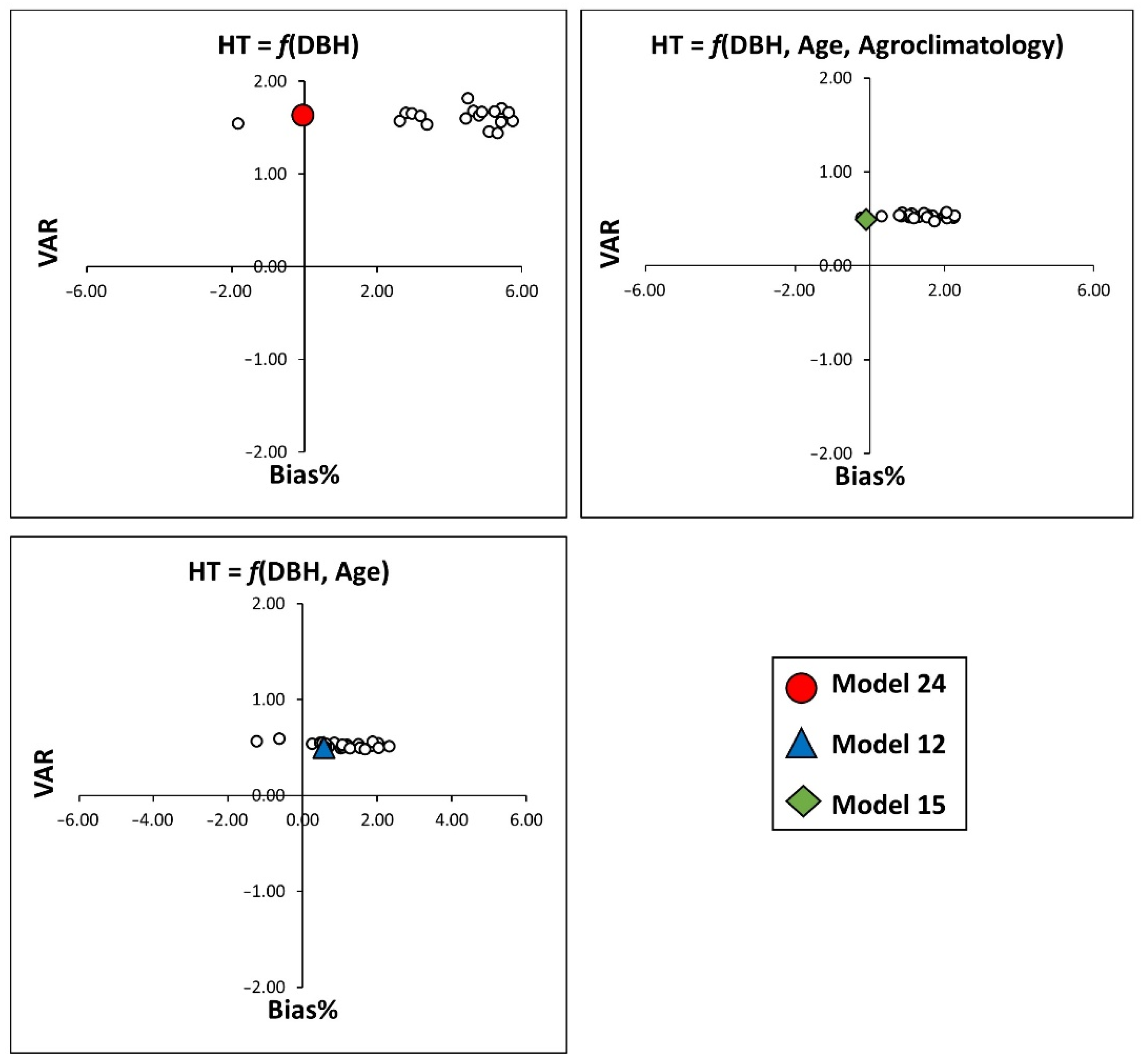
3.2. Model Validation Performance

We statistically analyzed each trained model with its respective function, evaluating the performance of RMSE, MAE for training, and we increased two more parameters for validation (Table 3). In general, all models with their responsive function showing a good performance. The HT = f(DBH) function showed a result that varies 1.26 ≤ RMSE ≤ 2.07 and 0.93 ≤ MAE ≤ 1.79 for training and 1.26≤ RMSE ≤ 2.06, 0.93 ≤ MAE ≤ 1.78, −1.84 ≤ Bias% ≤ 10.95 and 1.44 ≤ VAR ≤ 2.78 for validation. The function HT = f(DBH, Age) showed a result that varies 0.70 ≤ RMSE ≤ 0.78 and 0.49 ≤ MAE ≤ 0.57 for training and 0.71 ≤ RMSE ≤ 0.78, 0.49 ≤ MAE ≤ 0.57, −1.24 ≤ Bias% ≤ 2.32, 0.49 ≤ VAR ≤ 0.60 for validation. The function HT = f(DBH, Age, Agroclimatology) showed a result that varies 0.70 ≤ RMS E≤ 0.79 and 0.50 ≤ MAE ≤ 0.54 for training and 0.70 ≤ RMSE ≤ 0.79, 0.50 ≤ MAE ≤ 0.55, −0.23 ≤ Bias% ≤ 2.27 and 0.48 ≤ VAR ≤ 0.57 for validation.
To recognize the model of each function, we not only analyze the forecast Key Performance Indicator (KPI). We also analyze the residual plot; that is, the relative error in percentage between the predicted values (Figure 4) and the bias-variance tradeoff (Figure 5). According to the results, model 24 of the function HT = f(DBH) with RMSE = 1.26 and MAE = 0.93, model 12 of the function HT = f(DBH, Age) RMSE = 0.71 and MAE = 0.51, and model 15 of the function HT = f(DBH, Age, Agroclimatology) RMSE = 0.70 and MAE = 0.50, present a better performance than the others.

4. Discussion

4.1. Training Status for the Prediction of the Total Height of Bolaina Blanca

All the trained models did not need to complete the 300 number of epochs to converge the weights, because thanks to the regularization of early stopping the training of the models stopped as they did not present improvements in the validation metric, this method is not very intrusive and minimizes established metric across epochs [35], however stopping too early can enlarge bias and reduce variance, just as stopping too late can reduce bias and enlarge variance [36], that is why the importance of performing a hyperparameter optimization search with several trainings and observing the variance and bias compensation, adapting it for each type of problem [37]. In our study, model 5 of the HT = f(DBH) function needed the greatest number of epochs to converge the weights, with 195.7 epochs, and model 10 of the HT = f(DBH) function needed the least amount of epochs. to converge the weights with 5.4 epochs, which leads to a greater and lesser process of training time, respectively. However, model 24 of the function HT = f(DBH), model 12 of the function HT = f(DBH, Age) and model 15 of the function HT = f(DBH, Age, Agroclimatology) with 11.3, 10.7 and 11 number of epochs, respectively, present a better performance in their statistical evaluations than the rest (Table 3). Regarding its typology of number of neurons, the best networks of each function were 2 (50:50), 5 (50:25:5:25:50), and 2 (50:50), respectively, this is relatively dependent on In each study, in case of presenting too much information, more neurons will be needed to converge the weights [38] and more hidden layers in the model will be more complex or deep. The hidden layer activation function of the best performing models was maxout, the advantage of this hidden layer activation function is that the network learns the relationship between the hidden units and also the activation function of each hidden unit [35] but doubles the number of parameters for each neuron, which leads to a high total number of parameters [11], as shown in Table 2, the increase in the weights of the training used. This maxout function was initially presented as a natural companion using dropout to train convolutional networks, but studies have also been carried out without dropout as a substitute for the sigmoidal function and it has even been tested to solve regression problems, producing good results [39]. Although it is true, until the completion of this manuscript, that deep learning techniques have not been used for Bolaina Blanca tree height predictions, many studies have been conducted in other species using classical artificial neural network (ANN) techniques in other species, i.e., with a single hidden layer, in a large part of all these studies have been used with sigmoidal activation function, such as the hyperbolic and sigmoid tangent, obtaining satisfactory results [7,40,41,42]. The processing time of the modeling functions depends on the characteristics of the computer and is relative, however, the execution of our configurations for the height mode does not require a high demand on the characteristics of the computer from the user.

4.2. Growth and Estimation of the Total Height of Bolaina Blanca

In Peru, forestry and forest management of the species of Guazuma crinita Mart. It has been extensively studied since 1992 by Vidaurre and Héctor [43], evaluating its growth and the optimal sites for the development of the species. Subsequently, its economic importance is studied [44], becoming the dominant species for the sustenance of farmers in the Peruvian Amazon, initially opening up to a series of investigations, such as its geographical variation in its growth and wood density [45], modeling of its production [46]. However, it was not until 2018 that the total height of the species was modeled for the first time by Elera Gonzáles [47] in the Peruvian Amazon, in which she used regression techniques applying six hypsometric models, obtaining as a result of the performance of the models a range of 1.86 ≤ RMSE ≤ 1.93 and 1.44 ≤ MAE ≤ 1.52, it should be noted that these hypsometric models had a relationship of total height between DBH, DBH dominant and Age. In our study using a DNN, it exceeds the statistical performances (Table 3) and it is very likely that it also exceeds when ANN techniques are used, for smaller areas. When we analyzed the best configurations obtained in our study, the relationship between height and diameter, HT = f(DBH), the RMSE result was 1.26 (Model 24). The performance increases when we increase the relation between the DBH and age, HT = f(DBH, Age) with RMSE = 0.71 (Model 12) and even more when it is related to agroclimatic variables, HT = f(DBH, Age, Agroclimatology), with RMSE = 0.70 (Model 15). As we can see, obtaining a relationship between diameter and height in this species is relatively complex using regression techniques, and could even worsen if biased data were used, especially from inventories of plantation areas that have not received uniform forest management. The inclusion of climatological variables could bias the modeling for the prediction of the total height of the species (Figure 5), these directly influence decision-making for forest planning, such as silvicultural treatments, land acquisition, and genotype selection [48], in which various studies have shown better performance using agroclimatic variables, especially for growth and production models in eucalyptus plantations [49,50,51,52].
The models used in this study are efficient, both statistically and practically, as we highlight a specific configuration for each function used. We developed three functions to be adapted to different areas of the Peruvian Amazon, according to the database of each community. As the first function, we use only the diameter as an independent variable, being able to be considered as a guide for local communities with smaller-scale production, where plantations are not monitored (age or other variables of the forest mass). The second and third functions are for companies or cooperatives with medium or large-scale plantations, where permanent monitoring is carried out.
Extrapolation beyond the levels of the predictor variables, for example, dbh, will always have some risk, so the application to values outside the ranges observed in the study requires caution on the part of the reader in the application of the functions. However, although it may be a limitation, the range observed in the data covers a very large range of occurrences of values in the predictor variables, resulting in a great potential for the use of the proposed models. The study is a great contribution to the scientific community, farmers, and companies dedicated to the modeling and production of Guazuma crinita Mart. in the Peruvian Amazon.

5. Conclusions

The deep artificial neural network technique presents satisfactory performance for predictions of the total height of Guazuma crinite Mart. in modeling large areas. In general, all the variables used to influence the predictions. However, the addition of the agroclimatic variables together with the diameter at breast height and age have shown better accuracy than the others. Our hyperparameter configuration proposal (Model 24—HT = f(DBH), Model 12—HT = f(DBH, Age) and Model 15—HT = f(DBH, Age, Agroclimatology)) present the best performance and can be adapted to other forest management problems using a large amount of data. Likewise, we recommend carrying out studies with data from pre-cut inventories and with the addition of categorical variables.

Supplementary Materials

The following are available online at https://www.mdpi.com/article/10.3390/f13050697/s1, Table S1: Training status of each model and type of function evaluated used to predict the total height of Guazuma crinita Mart. in Peruvian amazon.

Author Contributions

Conceptualization, G.G.C. and H.G.L.; Formal analysis, D.G.E.G., J.R.B.V. and L.P.F.; Methodology, G.G.C. and H.G.L.; Writing—original draft, G.G.C.; Writing—review & editing D.G.E.G. and J.R.B.V. All authors have read and agreed to the published version of the manuscript.

Funding

This study was financed in part by the “Fundação de Amparo à Pesquisa do Estado de Minas Gerais—FAPEMIG”—Financing Code 507, and the “Coordenação de Aperfeiçoamento de Pessoal de Nível Superior, Brasil—CAPES”—Financing Code 001, in collaboration with the “Fundação Arthur Bernardes—FUNARBE”.

Institutional Review Board Statement

Not applicable.

Informed Consent Statement

Not applicable.

Data Availability Statement

Not applicable.

Acknowledgments

The authors are grateful to the “Fundação de Amparo à Pesquisa do Estado de Minas Gerais—FAPEMIG”, “Coordenação de Aperfeiçoamento de Pessoal de Nível Superior, Brasil—CAPES”, “Fundação Arthur Bernardes—FUNARBE”, Federal University of Viçosa and Reforestadora Amazónica S.A. company by providing the dataset utilized on this study and which constitute a major contribution to the Peruvian forestry sector, as well to the technical personnel and field workers of this company for the great work done in the data collection.

Conflicts of Interest

The authors declare that they have no conflict of interest.

References

  1. Álvarez Gómez, L.; Ríos Torres, S. Evaluación Económica de Parcelas de Regeneración Natural y Plantaciones de Bolaina Blanca, Guazuma crinita, En El Departamento de Ucayali; Instituto de Investigaciones de la Amazonía Peruana (IIAP): Iquitos, Peru, 2009; p. 54. [Google Scholar]
  2. Putzel, L.; Cronkleton, P.; Larson, A.; Pinedo-Vásquez, M.; Salazar, O.; Sears, R. Producción y Comercialización de Bolaina (Guazuma Crinita), Una Especie Amazónica de Rápido Crecimiento: Un Llamado a la Adopción de un Marco de Políticas que Apoye los Medios de Vida; Centro de Investigación Forestal Internacional (CIFOR): Bogor, Indonesia, 2013; p. 6. [Google Scholar]
  3. Reynel, C.; Pennington, R.; Pennington, T.; Flores, D.; Daza, C.A. Árboles Útiles de La Amazonía Peruana, Manual de Identificación Ecológica y Propagación de Las Especies; Herbario de la Facultad de Ciencias Forestales de la Universidad Nacional Agraria-La Molina, Royal Botanic Gardens Kew, Royal Botanic Gardens Edinburgh e ICRAF: Lima, Perú, 2003; ISBN 9972-9733-1-X. [Google Scholar]
  4. Tuisima-Coral, L.L.; Hlásná Čepková, P.; Weber, J.C.; Lojka, B. Preliminary Evidence for Domestication Effects on the Genetic Diversity of Guazuma crinita in the Peruvian Amazon. Forests 2020, 11, 795. [Google Scholar] [CrossRef]
  5. SERFOR (Servicio Nacional Forestal y de Fauna Silvestre) SNIFFS—Componente Estadístico. Available online: http://sniffs.serfor.gob.pe/estadistica/es/tableros/registros-nacionales/plantaciones (accessed on 11 March 2021).
  6. De Mendonça, A.R.; Corandin, C.M.; Pacheco, G.R.; Vieira, G.C.; Araújo, M.D.S.; Interamnense, M.T. Modelos Hipsométricos Tradicionais e Genéricos Para Pinus Caribaea Var. Hondurensis. Pesqui. Florest. Bras. 2014, 35, 47–54. [Google Scholar] [CrossRef] [Green Version]
  7. Da Rocha, J.E.C.; Junior, M.R.N.; Júnior, I.d.S.T.; de Souza, J.R.M.; Lopes, L.S.d.S.; da Silva, M.L. Configuração de Redes Neurais Artificiais Para Relação Hipsométrica de Árvores de Eucalyptus spp. Sci. For. 2021, 49, e3706. [Google Scholar] [CrossRef]
  8. Campos, J.C.C.; Leite, H.G. Mensuração Florestal: Perguntas e Respostas, 5th ed.; UFV: Viçosa, Brazil, 2017; ISBN 85-7269-579-6. [Google Scholar]
  9. Melo, E.d.A.; Calegario, N.; de Mendonça, A.R.; Possato, E.L.; Alves, J.d.A.; Isaac Júnior, M.A. Modelagem Não Linear Da Relação Hipsométrica e Do Crescimento Das Árvores Dominantes e Codominantes de Eucalyptus sp. Ciênc. Florest. 2017, 27, 1325–1338. [Google Scholar] [CrossRef] [Green Version]
  10. Rai, B. Advanced Deep Learning with R: Become an Expert at Designing, Building, and Improving Advanced Neural Network Models Using R; Packt Publishing Ltd.: Birmingham, UK, 2019; ISBN 978-1-78953-498-6. [Google Scholar]
  11. Aggarwal, C.C. Neural Networks and Deep Learning: A Textbook; Springer: Cham, Switzerland, 2018; ISBN 978-3-319-94462-3. [Google Scholar]
  12. LeCun, Y.; Bengio, Y.; Hinton, G. Deep Learning. Nature 2015, 521, 436–444. [Google Scholar] [CrossRef]
  13. Bergstra, J.; Bengio, Y. Random Search for Hyper-Parameter Optimization. J. Mach. Learn. Res. 2012, 13, 281–305. [Google Scholar]
  14. Hutter, F.; Lücke, J.; Schmidt-Thieme, L. Beyond Manual Tuning of Hyperparameters. KI-Künstl. Intell. 2015, 29, 329–337. [Google Scholar] [CrossRef]
  15. Claesen, M.; De Moor, B. Hyperparameter Search in Machine Learning. arXiv 2015, arXiv:1502.02127. [Google Scholar]
  16. Hutter, F.; Kotthoff, L.; Vanschoren, J. Automated Machine Learning: Methods, Systems, Challenges; Springer: Cham, Switzerland, 2019; ISBN 978-3-030-05317-8. [Google Scholar]
  17. Rodrigues de Oliveira, R.; Ferreira Rodrigues, L.; Mari, J.F.; Coelho Naldi, M.; Gomes Milagres, E.; Rocha Vital, B.; Oliveira Carneiro, A.d.C.; Breda Binoti, D.H.; Lopes, P.F.; Garcia Leite, H. Automatic Identification of Charcoal Origin Based on Deep Learning. Maderas Cienc. Tecnol. 2021, 23, 1–12. [Google Scholar] [CrossRef]
  18. Ferreira, M.P.; de Almeida, D.R.A.; de Almedia Papa, D.; Minervino, J.B.S.; Veras, H.F.P.; Formighieri, A.; Santos, C.A.N.; Ferreira, M.A.D.; Figueiredo, E.O.; Ferreira, E.J.L. Individual Tree Detection and Species Classification of Amazonian Palms Using UAV Images and Deep Learning. For. Ecol. Manag. 2020, 475, 118397. [Google Scholar] [CrossRef]
  19. Xi, Z.; Hopkinson, C.; Rood, S.B.; Peddle, D.R. See the Forest and the Trees: Effective Machine and Deep Learning Algorithms for Wood Filtering and Tree Species Classification from Terrestrial Laser Scanning. ISPRS J. Photogramm. Remote Sens. 2020, 168, 1–16. [Google Scholar] [CrossRef]
  20. Hamdi, Z.M.; Brandmeier, M.; Straub, C. Forest Damage Assessment Using Deep Learning on High Resolution Remote Sensing Data. Remote Sens. 2019, 11, 1976. [Google Scholar] [CrossRef] [Green Version]
  21. Bayat, M.; Bettinger, P.; Heidari, S.; Henareh Khalyani, A.; Jourgholami, M.; Hamidi, S.K. Estimation of Tree Heights in an Uneven-Aged, Mixed Forest in Northern Iran Using Artificial Intelligence and Empirical Models. Forests 2020, 11, 324. [Google Scholar] [CrossRef] [Green Version]
  22. da Silva, A.K.V.; Borges, M.V.V.; Batista, T.S.; da Silva Junior, C.A.; Furuya, D.E.G.; Prado Osco, L.; Teodoro, L.P.R.; Baio, F.H.R.; Ramos, A.P.M.; Gonçalves, W.N.; et al. Predicting Eucalyptus Diameter at Breast Height and Total Height with UAV-Based Spectral Indices and Machine Learning. Forests 2021, 12, 582. [Google Scholar] [CrossRef]
  23. Costa Filho, S.V.S.d.; Arce, J.E.; Montaño, R.A.N.R.; Pelissari, A.L. Tunning Machine Learning Algorithms for Forestry Modeling: A Case Study in the Height-Diameter Relationship. Ciênc. Florest. 2019, 29, 1501–1515. [Google Scholar] [CrossRef] [Green Version]
  24. Ercanli, İ. Artificial Intelligence with Deep Learning Algorithms to Model Relationships between Total Tree Height and Diameter at Breast Height. For. Syst 2020, 29, e013. [Google Scholar] [CrossRef]
  25. Ercanlı, İ. Innovative Deep Learning Artificial Intelligence Applications for Predicting Relationships between Individual Tree Height and Diameter at Breast Height. For. Ecosyst. 2020, 7, 12. [Google Scholar] [CrossRef] [Green Version]
  26. Casas, G.G.; Fardin, L.P.; Silva, S.; de Oliveira Neto, R.R.; Breda Binoti, D.H.; Leite, R.V.; Ramos Domiciano, C.A.; de Sousa Lopes, L.S.; da Cruz, J.P.; dos Reis, T.L.; et al. Improving Yield Projections from Early Ages in Eucalypt Plantations with the Clutter Model and Artificial Neural Networks. JST 2022, 30, 1257–1272. [Google Scholar] [CrossRef]
  27. Vendruscolo, D.G.S.; Chaves, A.G.S.; Medeiros, R.A.; da Silva, R.S.; Souza, H.S.; Drescher, R.; Leite, H.G. Height Estimative of Tectona Grandis, L. f. Trees Using Regression and Artificial Neural Networks. Nativ. Pesqui. Agrár. Ambient. 2017, 5, 52–58. [Google Scholar] [CrossRef] [Green Version]
  28. Binoti, D.H.B.; Duarte, P.J.; Silva, M.L.M.d.; Silva, G.F.d.; Leite, H.G.; Mendonça, A.R.d.; Andrade, V.C.L.D.; Vega, A.E.D. Estimation of Height of Eucalyptus Trees with Neuroevolution of Augmenting Topologies (Neat). Rev. Árvore 2018, 41, e410314. [Google Scholar] [CrossRef]
  29. Gobernador Regional de Huánuco. GRH-Gobierno Regional de Huánuco Zonificación Ecológica Económica Base Para El Ordenamiento Territorial de La Región Huánuco; Gobernador Regional de Huánuco: Huánuco, Peru, 2016; p. 260. [Google Scholar]
  30. Holdridge, L.R. Tropical Science Center: San jose, Costa Rica. In Life Zone Ecology; Tropical Science Center: San Jose, Costa Rica, 1967. [Google Scholar]
  31. LeDell, E.; Gill, N.; Aiello, S.; Fu, A.; Candel, A.; Click, C.; Kraljevic, T.; Nykodym, T.; Aboyoun, P.; Kurka, M.; et al. H2O: R Interface for the “H2O” Scalable Machine Learning Platform; R Foundation for Statistical Computing: Vienna, Austria, 2020. [Google Scholar]
  32. Team, R.C. R: A Language and Environment for Statistical Computing; R Foundation for Statistical Computing: Vienna, Austria, 2020. [Google Scholar]
  33. Zeiler, M.D. Adadelta: An Adaptive Learning Rate Method. arXiv 2012, arXiv:1212.5701. [Google Scholar]
  34. Islam, M.; Kurttila, M.; Mehtätalo, L.; Haara, A. Analyzing the Effects of Inventory Errors on Holding-Level Forest Plans: The Case of Measurement Error in the Basal Area of the Dominated Tree Species. Silva Fenn. 2009, 43, 71–85. [Google Scholar] [CrossRef] [Green Version]
  35. Goodfellow, I.J.; Warde-Farley, D.; Mirza, M.; Courville, A.; Bengio, Y. Maxout Networks. In Proceedings of the International Conference on Machine Learning, Atlanta, GA, USA, 16–21 June 2013; Volume 28, p. 9. [Google Scholar]
  36. Yao, Y.; Rosasco, L.; Caponnetto, A. On Early Stopping in Gradient Descent Learning. Constr. Approx. 2007, 26, 289–315. [Google Scholar] [CrossRef]
  37. Naik, D.L.; Sajid, H.U.; Kiran, R.; Chen, G. Detection of Corrosion-Indicating Oxidation Product Colors in Steel Bridges under Varying Illuminations, Shadows, and Wetting Conditions. Metals 2020, 10, 1439. [Google Scholar] [CrossRef]
  38. Binoti, D.H.B.; Binoti, M.L.M.S.; Leite, H.G. Configuração de Redes Neurais Artificiais Para Estimação Do Volume de Árvores. Rev. Ciênc. Madeira-RCM 2014, 5, 58–67. [Google Scholar] [CrossRef]
  39. Jakobsson, E. Applying the Maxout Model to Increase the Performance of the Multilayer Perceptron in Shallow Networks. Bachelor’s Thesis, Lund University, Lund, Sweden, 2016. [Google Scholar]
  40. Martins, E.R.; Binoti, M.L.M.S.; Leite, H.G.; Binoti, D.H.B.; Dutra, G.C. Configuration of Artificial Neural Networks for Estimation of Total Height of Eucalyptus Trees. Agraria 2016, 11, 117–123. [Google Scholar] [CrossRef] [Green Version]
  41. Dantas, D.; Rodrigues Pinto, L.O.; de Castro Nunes Santos Terra, M.; Calegario, N.; Romarco de Oliveira, M.L. Reduction of Sampling Intensity in Forest Inventories to Estimate the Total Height of Eucalyptus Trees. Bosque Vald. 2020, 41, 353–364. [Google Scholar] [CrossRef]
  42. Silva, S.; de Oliveira Neto, S.N.; Leite, H.G.; de Alcântara, A.E.M.; de Oliveira Neto, R.R.; de Souza, G.S.A. Productivity Estimate Using Regression and Artificial Neural Networks in Small Familiar Areas with Agrosilvopastoral Systems. Agrofor. Syst. 2020, 94, 2081–2097. [Google Scholar] [CrossRef]
  43. Vidaurre, A.; Héctor, E. Silvicultura y Manejo de Guazuma crinita Mart.; Instituto Nacional de Investigación Agraria y Agroindustrial-INIAA: Ucayali, Peru, 1992. [Google Scholar]
  44. Gonzales Ego-Aguirre, L.A. Evaluación Técnico-Económica de Plantaciones de Bolaina Blanca (Guazuma crinita Mart.) En Zonas Inundables Del Río de Aguaytía. Ph.D. Thesis, Universidad Nacional Agraria La Molina, Lima, Peru, 2003. [Google Scholar]
  45. Weber, J.C.; Sotelo Montes, C. Geographic Variation in Tree Growth and Wood Density of Guazuma crinita Mart. in the Peruvian Amazon. New For. 2008, 36, 29–52. [Google Scholar] [CrossRef]
  46. Guerra, W.; Soudre-Zambrano, M.; Chota, M. Tabla de Volumen Comercial de Bolaina Blanca (Guazuma crinita Mart.) de Las Plantaciones Experimentales de Alexander Von Humboldt, Ucayali, Perú. Folia Amaz. 2008, 4, 47. [Google Scholar] [CrossRef] [Green Version]
  47. Elera Gonzáles, D.G. Modeling of Growth and Spatialization of the Productive Capacity of Bolaina (Guazuma crinita Mart.) Plantations on Peruvian Central Amazon. Ph.D. Thesis, Universidade Federal de Viçosa, Viçosa, Brazil, 2018. [Google Scholar]
  48. Scolforo, J.R.S.; Maestri, R.; Ferraz Filho, A.C.; de Mello, J.M.; de Oliveira, A.D.; de Assis, A.L. Dominant Height Model for Site Classification of Eucalyptus Grandis Incorporating Climatic Variables. Int. J. For. Res. 2013, 2013, 139236. [Google Scholar] [CrossRef] [Green Version]
  49. Alcantra, A.E.M.d.; Santos, A.C.d.A.; Silva, M.L.M.d.; Binoti, D.H.B.; Soares, C.P.B.; Gleriani, J.M.; Leite, H.G. Use of Artificial Neural Networks to Assess Yield Projection and Average Production of Eucalyptus Stands. Afr. J. Agric. Res. 2018, 13, 2285–2297. [Google Scholar] [CrossRef] [Green Version]
  50. Medeiros, R.A.; Paiva, H.N.d.; Soares, Á.A.V.; Marcatti, G.E.; Takizawa, F.H.; Domiciano, C.A.R.; Leite, H.G. Productive Potential of Tectona Grandis in Midwest Brazil. Adv. For. Sci. 2019, 6, 803. [Google Scholar] [CrossRef]
  51. Freitas, E.C.S.d.; Paiva, H.N.d.; Neves, J.C.L.; Marcatti, G.E.; Leite, H.G. Modeling of Eucalyptus Productivity with Artificial Neural Networks. Ind. Crop. Prod. 2020, 146, 112149. [Google Scholar] [CrossRef]
  52. De Oliveira Neto, R.R.; Leite, H.G.; Gleriani, J.M.; Strimbu, B.M. Estimation of Eucalyptus Productivity Using Efficient Artificial Neural Network. Eur. J. For. Res. 2022, 141, 129–151. [Google Scholar] [CrossRef]
Figure 1. Location of the study and the forest plantations area of Guazuma crinita Mart. (A) in the Province of Puerto Inca (B), Department of Huánuco (C), Peruvian Amazon.
Forests 13 00697 g001
Figure 2. Number of neurons or units in the hidden layer used for hypsometric modeling of the Guazuma crinita Mart. in the Peruvian Amazon. The numbers of neurons in the hidden layer were 10:10 (A), 10:5 (B), 10:5:2 (C), 50:50 (D), 50:25 (E), 50:25:5 (F), 10: 5:2:5:10 (G), and 50:25:5:25:50 (H).
Forests 13 00697 g002
Figure 3. Methodological flow diagram established in our study for the hypsometric modeling of Guazuma crinita Mart. trees in the Peruvian Amazon.
Forests 13 00697 g003
Figure 4. Residual graph in relation to the predicted total height for the hypsometric modeling of the trees of Guazuma crinita Mart. in the Peruvian Amazon, for each trained model and based on the three study functions: HT = f(DBH), HT = f(DBH, Age) and HT = f(DBH, Age, Agroclimatology).
Forests 13 00697 g004
Figure 5. Graph of the relationship between bias and variance for the hypsometric modeling of Guazuma crinite Mart. trees in the Peruvian Amazon, showing with greater emphasis the best trained model for each of the three study functions: HT = f(DBH), HT = f(DBH, Age) and HT = f(DBH, Age, Agroclimatology).
Forests 13 00697 g005
Table 1. Descriptive statistics of the dendrometric and agroclimatic variables of the Guazuma crinita Mart. in the Peruvian Amazon.
Descriptive Statistics
DendrometricMeanMinimumMaximumVarianceStd.Dev.Coef.Var.
Age (years)2.560.407.301.631.2849.92
DBH (cm)10.700.5029.6020.224.5042.01
HT (m)11.053.0025.8222.634.7643.03
Agroclimatic
Surface Pressure (kPa)97.5297.4797.560.000.030.03
Temperature at 2 Meters (°C)26.9826.4028.470.450.672.49
Specific Humidity at 2 Meters (g/kg)16.0815.0117.150.470.684.25
Relative Humidity at 2 Meters (%)73.0763.0078.3123.924.896.69
Wind Speed at 2 Meters (m/s)0.060.050.090.000.0229.51
Surface Soil Wetness0.610.500.700.000.069.73
Temperature at 2 Meters Maximum (°C)39.1038.0939.730.450.671.71
Temperature at 2 Meters Minimum (°C)18.2917.3319.240.400.633.45
Profile Soil Moisture0.660.620.720.000.034.39
Root Zone Soil Wetness0.650.620.720.000.034.67
Wind Speed at 2 Meters Maximum (m/s)0.660.550.730.000.079.89
Wind Speed at 10 Meters Maximum (m/s)2.182.042.300.010.115.14
Wind Speed at 10 Meters Minimum (m/s)0.020.010.030.000.0137.80
Precipitation Corrected (mm/day)3.011.754.370.570.7625.12
Wind Speed at 10 Meters Range (m/s)2.162.012.270.010.115.02
All Sky Surface UVA Irradiance (W/m2)11.7111.4012.030.050.221.89
All Sky Surface UVB Irradiance (W/m2)0.350.340.360.000.012.65
All Sky Surface Shortwave DownwardIrradiance (MJ/m2/day)16.1915.6316.560.120.352.16
Clear Sky Surface Shortwave DownwardIrradiance (MJ/m2/day)24.0723.8124.230.030.180.73
All Sky Surface PAR Total (W/m2) 87.5884.6589.743.281.812.07
Clear Sky Surface PAR Total (W/m2)128.36126.02129.621.481.220.95
Table 2. State and architecture of each model trained according to the three functions evaluated for the predictions of the total height of the Guazuma crinita Mart. trees in the Peruvian Amazon.
ModelHidden LayerEpochs/Training Samples/Weights and BiasesTotal Layers
Activation FunctionsLayers/UnitsHT = f(DBH)HT = f(DBH, Age)HT = f(DBH, Age, Agroclimatology)
Model 1Tanh2(10:10)34.9/3,300,864/15135/3,307,955/16117.4/1,647,234/3714
Model 2Rectifier2(10:10)89.9/8,496,703/15160.3/5,700,023/16130/2,835,773/3714
Model 3Maxout2(10:10)65/6,145,912/29141/3,872,041/31125.1/2,369,990/7314
Model 4Tanh2(10:5)64.5/6,100,250/9148.7/4,599,721/10117.1/1,614,741/3114
Model 5Rectifier2(10:5)195.7/18,497,950/91159.8/15,100,404/10130.4/2,869,197/3114
Model 6Maxout2(10:5)51.7/4,882,319/17662.4/5,897,233/19625/2,358,105/6164
Model 7Tanh3(10:5:2)70.9/6,698,582/10073/6,901,805/11032.9/3,108,612/3205
Model 8Rectifier3(10:5:2)92.1/8,702,945/100148.1/14,000,065/11030.6/2,892,184/3205
Model 9Maxout3(10:5:2)85.7/8,097,387/19777/7281,256/21721.7/2,051,691/6375
Model 10Tanh2(50:50)5.4/509,363/27516.7/637,904/28017.9/744,223/38514
Model 11Rectifier2(50:50)44.5/4,207,558/275127.7/2,615,333/280111.6/1,093,767/38514
Model 12Maxout2(50:50)10.7/1,007,812/545110.7/1,008,106/555110.8/1,023,225/76514
Model 13Tanh2(50:25)9.7/917,479/145113.2/1,251,731/15015.7/542,308/25514
Model 14Rectifier2(50:25)37.5/3,547,655/145123.9/2,260,683/150112/1,132,858/25514
Model 15Maxout2(50:25)13/1,230,927/28769.4/885,209/297611/1,035,577/50764
Model 16Tanh3(50:25:5)7.9/748,206/15618.9/843,398/16118.3/783,786/26615
Model 17Rectifier3(50:25:5)41.7/3,939,088/156123.6/2,226,682/161120/1,893,917/26615
Model 18Maxout3(50:25:5)23.4/2,215,252/31169.6/907,092/32169.1/857,062/53165
Model 19Tanh5(10:5:2:5:10)54/5,103,702/18353/5,009,328/19344.4/4,197,664/4037
Model 20Rectifier5(10:5:2:5:10)160.8/15,202,054/18365.6/6,200,261/19339.6/3,738,971/4037
Model 21Maxout5(10:5:2:5:10)42.3/4,001,607/35535.2/3,328,508/37523.7/2,240,775/7957
Model 22Tanh5(50:25:5:25:50)10.1/955,656/30568/760,293/31066.3/598,638/41567
Model 23Rectifier5(50:25:5:25:50)29.3/2,766,703/305635.7/3,369,835/310612.3/1,160,523/41567
Model 24Maxout5(50:25:5:25:50)11.3/1,072,656/606113.9/1,309,262/616110.5/996,059/82617
Table 3. Performance of the statistics of each model trained and function evaluated, both for training and for validation in the total height predictions of the Guazuma crinita Mart. in the Peruvian Amazon.
HT = f(DBH)HT = f(DBH, Age)HT = f(DBH, Age, Agroclimatology)
TrainValidationTrainValidationTrainValidation
ModelRMSEMAERMSEMAEBias%VARRMSEMAERMSEMAEBias%VARRMSEMAERMSEMAEBias%VAR
Model 11.421.191.431.26.041.610.780.570.770.57−0.630.60.760.520.760.521.670.54
Model 21.461.231.471.246.321.670.760.530.750.520.840.550.760.520.760.521.110.56
Model 31.381.131.41.144.651.680.750.520.740.511.180.530.760.530.760.532.230.51
Model 41.421.171.441.194.51.820.740.510.730.510.240.540.750.520.760.521.520.55
Model 51.391.141.411.165.741.580.780.540.770.532.020.550.770.530.760.530.850.57
Model 61.41.151.421.175.381.660.770.540.760.532.320.520.770.540.760.541.990.54
Model 71.321.051.321.062.781.660.750.510.750.511.490.540.730.510.740.511.30.52
Model 81.381.121.391.134.811.640.720.50.710.51.020.50.780.540.770.541.440.56
Model 91.41.151.431.175.431.670.750.530.750.521.850.520.730.510.740.511.020.53
Model 101.291.041.291.043.381.540.730.530.730.531.520.50.740.520.740.521.520.52
Model 111.431.191.441.195.431.710.730.50.740.511.210.520.750.540.750.532.060.51
Model 121.321.11.331.115.081.460.720.520.710.510.580.50.730.530.730.531.050.52
Model 131.311.041.331.052.961.660.720.510.720.511.070.510.790.540.770.542.270.54
Model 141.341.091.361.14.451.610.740.520.750.530.460.550.780.540.790.542.030.57
Model 151.391.141.391.135.431.560.720.510.720.511.670.490.70.50.70.5−0.090.49
Model 161.281.041.291.042.631.580.720.520.720.510.70.510.720.50.730.51.050.52
Model 171.411.151.421.155.241.680.770.520.780.531.870.560.780.540.790.552.050.57
Model 181.311.081.341.15.321.440.730.550.740.551.060.530.750.520.750.521.040.54
Model 192.071.792.061.7810.952.780.750.530.750.530.520.560.740.520.730.510.310.53
Model 201.311.041.331.043.21.630.740.530.740.520.610.540.750.520.730.510.830.53
Model 211.441.211.431.25.631.670.770.570.770.57−1.240.570.730.520.720.521.180.51
Model 221.280.961.280.95−0.041.630.70.50.710.50.610.50.740.520.740.510.780.54
Model 231.411.131.41.124.91.670.720.490.720.491.250.50.730.520.720.52−0.230.52
Model 241.260.931.260.93−1.841.550.760.520.740.522.030.50.720.50.720.51.730.48
Publisher’s Note: MDPI stays neutral with regard to jurisdictional claims in published maps and institutional affiliations.

