Shifting Importance of Abiotic versus Biotic Filtering from Intact Mature Forests to Post-Clearcut Secondary Forests

Abstract

Although ecologists often emphasize the roles of environmental- versus biotic-filtering in structuring forest communities, the relative importance of these processes could vary among undisturbed versus disturbed forests. To test this assumption, we gathered leaf traits and site conditions data from intact mature forests (control), moderately disturbed shrublands, and severely disturbed plantations from subtropical China. We found that plantations had higher leaf area, specific leaf area, leaf nitrogen and phosphorus concentrations but lower leaf thickness, dry matter content, and C:N than the shrubland or mature forest, suggesting the dominance of resource acquisition strategy in plantations versus conservation strategy in the mature forests. Plantations also had significantly lower trait ranges than mature forest or shrubland, suggesting the play of stringent environmental filtering in the plantation. However, intraspecific trait variations in leaf dry matter content and C:N were substantial in plantation, while interspecific variation in leaf thickness was high in mature forests, suggesting the importance of intra- versus inter-specific competition in plantation versus mature forests. Results from our species-level analysis were consistent with the community-level results mentioned above. Overall, our study demonstrates the shifting importance of environmental and biotic filtering from disturbed to undisturbed forests.

1. Introduction

Understanding community assembly or biodiversity maintenance processes across natural to human-modified systems is a central topic in ecology and is germane to anthropogenic land management [1,2,3,4]. Traditionally, ecologists describe community assembly as a sequential process: that is, species from a regional species pool first arrive at the locality; second, if the underlying environmental conditions suit, the arriving species survive; and finally, superior competitors among the surviving species make up the local community [5]. However, ecological processes rarely act individually or sequentially as such: processes often interact [6], and most importantly, the relative importance of processes may vary with site abiotic and biotic conditions [1]. Since anthropogenic habitat disturbances often modify site abiotic and biotic conditions, the importance of processes shaping ecological communities may vary among undisturbed versus disturbed habitats [7]. Yet, studies comparing community structuring processes for natural versus anthropogenically modified secondary forests are rare, especially in the context of natural versus post-clearcut secondary forests in the subtropics [7]. This is a significant knowledge gap with profound management implications, given that clearcutting is a relatively common forestry practice in the subtropics [8].

However, clearcutting practice itself can be of diversified forms [9,10]. Some forms of clearcutting involve removing all standing vegetation, followed by plantation raising. Other forms include removing commercially valuable (e.g., timber, pole, and fuelwood) stems and keeping the residual ground vegetation without any plantation raising. Such a contrasting approach to clearcutting often leads to different types of secondary forests, including plantation forests and shrublands in subtropical China [11,12]. Presumably, the relative importance of environmental versus biotic filtering structuring among post-disturbance and undisturbed forest communities might differ markedly. More specifically, in a post-clearcut plantation forest without residual ground vegetation, the planted and naturally colonized species often find the underlying environment severe [13], suggesting the possible play of stringent environmental filtering [14]. At that time, the number of resident or planted species should be relatively small, indicating somewhat weak biotic filtering mediated by interspecific competition [7]. However, intraspecific competition-mediated biotic filtering could be vital if the planted species are densely packed or crowded.

In contrast, if clearcutting does not remove the ground layer, such as the context of Chinese shrubland, the already adapted residual species of a post-clearcut secondary forest may experience the underlying environment somewhat less severe [10]. That means environmental filtering may be less intense. At the same time, removing the overstory trees through clearcutting may offer favorable conditions, allowing new species colonization and an increasing abundance of residual species [13], ultimately promoting interspecific competition. In sharp contrast to post-clearcut communities, species in undisturbed mature forests (control) usually adapt to the locality, experience productive environmental conditions, new species colonize, and the community becomes complex [15,16]. In that scenario, interspecific competition-mediated biotic filtering is crucial. In sum, the importance of interspecific competition-mediated biotic filtering should wane, and environmental filtering should strengthen with the increasing intensity of clearcutting disturbance.

One of the ways to verify such predictions is to employ a trait-based approach [6,17] and examine the patterns of trait mean, range, variation, and trait–trait covariation. While the mean, range, and covariation of traits can indicate the importance of environmental filtering, inter and intraspecific trait variations can show the importance of both biotic and environmental filtering. That is, plants that can tolerate a site’s abiotic condition should pass the environmental filter [18], share common phenotypic traits [3], and exhibit similarities in their trait values [17,19]. So, trait ranges (difference between the maximum and minimum trait values) should be narrow under robust environmental filtering and vice versa [3]. The overall values of trait mean (community-weighted) could be small or large depending on whether the underlying environment favors a small versus large phenotype or any particular functional strategy such as resource acquisition versus resource conservation. Trait–trait covariation should be strong under stringent environmental filtering because a species needs to fulfill a rigid set of multi-trait combinatorial criteria to earn community membership [20,21]. Therefore, if our hypothesis that environmental filtering may strengthen with increasing disturbance held, we should find a narrow trait range and higher trait–trait covariation in post-clearcut secondary forests versus intact mature forests. Similarly, we expect higher community-weighted mean values for resource acquisition trait (e.g., larger leaf area, higher specific leaf area, and higher leaf nitrogen and phosphorus concentrations) and lower values for resource conservation trait (e.g., leaf dry matter content, leaf thickness, leaf carbon to nitrogen ratio, and nitrogen to phosphorus ratio) in the in post-clearcut secondary forests than intact mature forests.

In contrast, the internal-biotic filter usually refers to the degree of inter and intraspecific competition among coexisting species [6], essentially limiting functional similarity [22]. Inter and intraspecific trait variations, which are signs of competition-mediated functional dissimilarity, could indicate the strength of internal-biotic filtering [23,24,25]. Consequently, if our assumption—that is, interspecific competition-mediated biotic filtering may weaken with disturbance—held, we should find more interspecific trait variation in intact mature forests than post-clearcut secondary forests. Alternatively, if post-disturbance plantation forests are densely packed and crowded, we may discover higher intraspecific trait variation due to intraspecific competition [25].

However, a community is a mixture of species, and it is the individual species that ultimately experience environmental filtering or competition. So, species’ attributes (i.e., trait mean and range) can offer complementary insights into biodiversity maintenance processes [17,26]. One crucial aspect of the species-level analysis is that a species’ trait values can be divided into within- and among-community components [17]. The within-community component, commonly denoted as alpha-trait value, describes how the trait value of a focal species relative to coexisting species varies; thus attributed to competition-mediated biotic filtering. The among-community component, denoted as beta-trait value, describes the mean-trait values of the focal species across communities; thus attributed to site condition-mediated environmental filtering. Therefore, a species experiencing robust biotic filtering should have a higher alpha-trait value, while a species facing robust environmental filtering should have a higher beta-trait value. So, in the context of post-clearcut secondary forest, we can hypothesize that most species occurring in the post-clearcut plantation forest would have higher beta-trait values, while most intact mature forests would have higher alpha-trait values. However, when a species occurs in a wide range of environmental conditions, its trait values should vary widely. The difference between maximum and minimum trait values for a species may thus indicate the species’ niche breadth. The more benign the environment is, the higher the niche breadth. So, species with higher niche breadth might dominate the intact mature forests more than the post-clearcut secondary forests.

The subtropical forest communities of eastern China include both intact mature forests and post-clearcut secondary forests (e.g., shrubland and plantation forests), offering a unique setting to assess external versus internal filters’ roles in undisturbed versus disturbed forest communities using a trait-based approach. Here forest disturbance takes the form of forest clearance through cutting for firewood. The cutting intensity has been severe, with the mature forest cleared but with many stumps remaining and then allowed to regrow [12]—the shrublands developed through natural regeneration after cessation of clearcutting [11]. In more intensively clear-cut areas, entire vegetation was removed and planted with Chinese fir and bamboo. By contrast, mature evergreen broadleaved climax forest had no history of cutting. While past research has assessed species and functional diversity patterns in these systems [27,28,29,30,31], mechanistic understanding regarding community assembly processes remains unclear. Therefore, this study utilizes mature forest, shrubland, and plantation communities that share a regional species pool and employ a trait-based approach to address the following three questions:

• Do community-level trait means, trait ranges, and trait–trait covariation reflective of external-environmental filtering vary among intact mature forest versus post-clearcut secondary forests?
• Do community-level inter and intraspecific trait variation reflective of biotic filtering vary among intact mature forest versus post-clearcut secondary forests?
• Do species-level alpha- and beta-trait values, as well as niche breaths, vary among intact mature forests versus post-clearcut secondary forests?

2. Materials and Methods

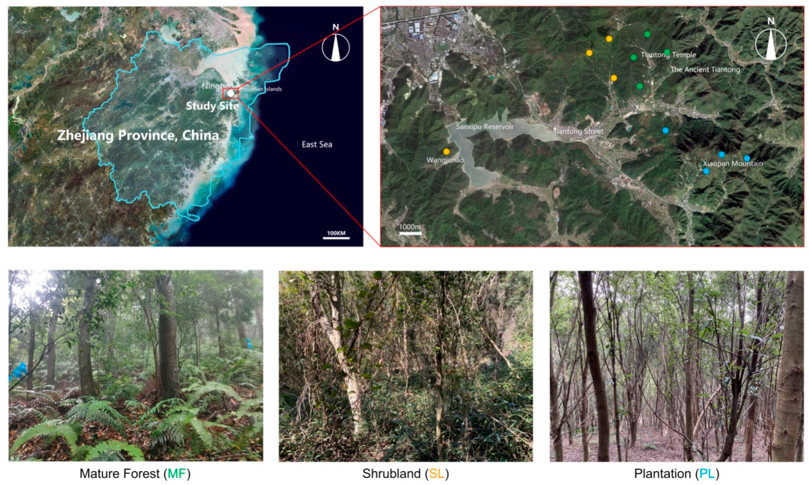
2.1. Study System and Natural History

This study was conducted in the subtropical forests at Tiantong National Forest Park of Eastern China (29°48′ N, 121°47′ E; elevation: 143–409 m a.s.l.; Figure 1). The regional climate is characterized by mean annual precipitation of 1679.42 mm and the mean annual temperature of 17.74 °C [32]. Topography is hilly, and soils are ferrallisols, rich in iron and aluminum oxides [21]. The climate and topographic conditions are ideal for typical subtropical evergreen forests. The overstory layer is dominated by Schima superba, Cyclobalanopsis myrsinaefolia, and Symplocos sumuntia; the shrub layer is dominated by Camellia fraternal, Loropetalum chinense, and Eurya muricate; and the ground layer is dominated by Cibotium barometz, Diplopterygium glaucum, and Dryopteris montigena.

The regionally famous Tiantong temple is located in this area, and the mature forest around the temple remains relatively intact, without any history of clearcutting. However, some forests around the temple were clearcut around 35 years ago for firewood. Those forests are now characterized by tall shrubs developed through natural regeneration after cessation of clearcutting [11]. Moreover, park authorities had clearcut the vegetation in some areas and raised large-scale plantations with Chinese fir decades ago. Many plant communities have recommenced the early stages of succession, which results in a very diverse mosaic of communities [12]. Thus, the study area includes relatively intact mature forest (MF), post-clearcut (with residual vegetation) shrubland (SL), and post-clearcut (without residual vegetation) plantation (PL) (Figure 1). The ages of the mature forest are over 60 years, shrublands are over 35 years, and plantations are around 20 years [29,33]. This 20–35 years time frame may be sufficient for vegetation restoration and recovery and thus suitable for assessment of assembly processes [8,9].

2.2. Sampling Design

We selected four sites from each of three forest types—post-clearcut plantation, post-clearcut shrubland, and intact mature forest—for a total of 12 sites in this study. Selected sites were separated from each other by at least 150 m. At each site (N = 12), we established six contiguous plots of 20 × 20 m for a total of 72 plots (6 plots per site × 4 sites per disturbance and control × 3 disturbance types = 72 × 20 × 20 m plots) in this study. We established six contiguous plots instead of six random plots to capture essential within-site variability in environmental properties, species, and functional composition. At the same time, we chose four sites per forest type to capture landscape-level between-site variations in environmental properties and species and functional composition.

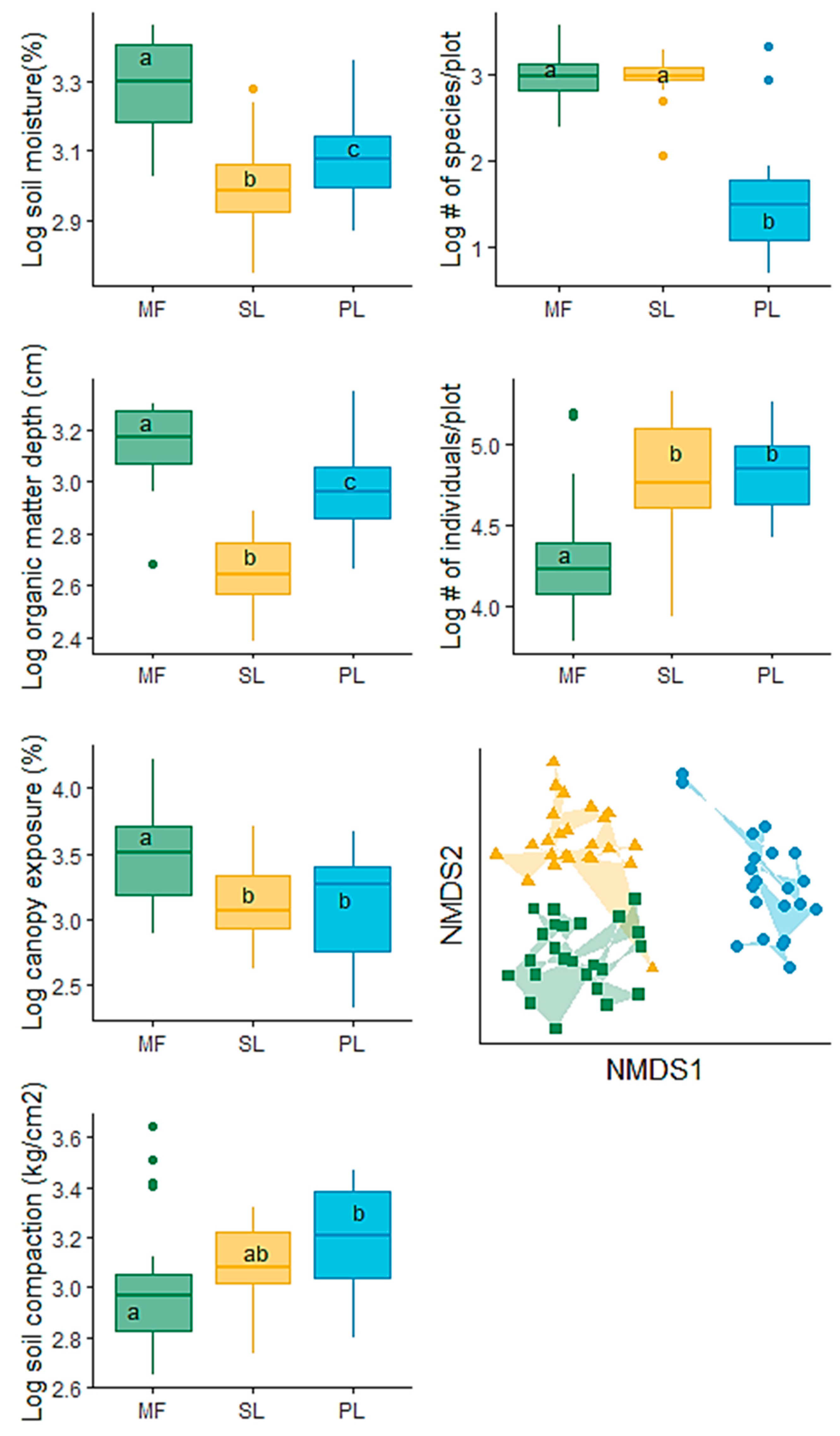
2.3. Vegetation and Environmental Data

We identified all woody species at each plot (N = 72) and recorded their abundance (i.e., counted the number of individuals). To assess the site’s environmental conditions, we measured (i) soil moisture content (%), (ii) the depth of organic matter (cm), (iii) canopy opening (%), and (iv) soil compaction (kg/cm²) at each plot. We measured soil moisture using an HH2 moisture meter (Delta-T Devices Ltd., Cambridge, England), soil organic matter depth using a hand-held auger, and soil compaction using a soil compaction meter (TJSD-750; Zhejiang Top Cloud-Agri Technology Co., Ltd., Hangzhou, China). We estimated canopy exposure ocularly (without using any instrument) on a 0–100% scale. For all environmental variables, except canopy exposure, we took five measurements at five random locations within a 20 × 20 m plot and averaged them to represent the plot. All environmental variables were measured within seven days without rain at least seven days before the measurement days.

2.4. Functional Traits

We focused on eight leaf traits: (i) leaf area (LA), (ii) specific leaf area (SLA), (iii) leaf dry matter content (LDMC), (iv) leaf thickness (LT), (v) leaf nitrogen concentration (LNC), (vi) leaf phosphorus concentration (LPC), (vii) leaf carbon to nitrogen ratio (C:N), and (viii) leaf nitrogen to phosphorus ratio (N:P) in this study. These traits represent essential physiological functions related to species performance, fitness, and distribution: LA and SLA are related to the plant growth rate [34,35]; LDMC is related to plant nutrient conservation [36]; LT is related to plant nutrient conservation, response to water deficits, and palatability to herbivores [37,38,39,40,41]; LNC and LPC concentrations are related to photosynthesis [42] and protein synthesis [43]; leaf C:N ratio is pertinent to plants’ nitrogen [44], whereas leaf N:P ratio is pertinent to phosphorous use efficiency and are usually negatively correlated with plant growth [45,46]. Correlations among the eight leaf traits were relatively weak (see Supplementary Materials, Section S1), implying that these traits may capture relatively unique information.

We measured leaf physical traits (LA, SLA, LDMC, and LT) for each species from three individuals at the plot level. If a species had less than three individuals in a plot, we collected trait data from all individuals. However, for leaf chemical traits (LNC, LPC, C:N, and N:P), we measured traits from a single individual from a 20 × 20 m² plot for logistical constraints. Hence, our sampling effort was robust enough to capture the interspecific trait variation for all traits at a resolution of plot-level and intraspecific trait variations at a resolution of site-level. We followed standard protocol for trait sampling [47,48]. That is, from each individual, we collected three well-grown branches with their leaves on them. Then, we selected 10 mature leaves without any sign of physical damage from each branch and combined all leaves to form a composite sample of over 60 leaves per individual. We wrapped these leaves in moist paper, placed them into a sealed plastic bag, and kept those bags in a cooler until they were transported back to the laboratory within six hours. Next, we randomly selected 10 mature leaves from each individual to weigh fresh leaf weight (l_fw) using an electric balance (BSA224S electronic scale, Sartorius Group, Beijing) and to measure leaf areas (l_area) using a leaf area meter (Li-Cor 3100C leaf area scanner, Li-Cor, Lincoln, NE, USA). Samples were then placed in an oven at 75 °C for 48 h to determine dry leaf weight (l_dw). We quantified SLA as l_area/l_dw, LDMC as l_dw/l_fw [47,48]. Leaf samples were then boiled with concentrated H₂SO₄ and H₂O₂ to oxidize and decompose leaf organic nitrogen and phosphorus. After the constant volume of dissolving solution, leaf nitrogen concentration (LNC) was assessed following Kjeldahl method [49], leaf phosphorus concentration (LPC) was assessed following the Mo-Sb Anti spectrophotometric method [50]. Leaf carbon concentration (LCC) was assessed following potassium dichromate oxidation outside the heating method [51].

2.5. Quantifying Plot- and Species-Level Trait Mean, Range, Variation, and Trait–Trait Covariation

To quantify plot-level community-weighted mean (P_j) and trait range (R_j) values for each trait, we followed Ackerly and Cornwell [17]. Utilizing the same approach, we quantified species-level trait mean (t_i), alpha-trait value (α_i), beta-trait value (β_i) and niche breadth (R_i) for each trait and species. The variables were computed as follows:

$$P_j=\frac{{{\displaystyle \sum }}_{i=1}^S{a}_{ij}{t}_{ij}}{{{\displaystyle \sum }}_{i=1}^S{a}_{ij}}$$

(1)

$$t_i=\frac{{{\displaystyle \sum }}_{j=1}^P{a}_{ij}{t}_{ij}}{{{\displaystyle \sum }}_{j=1}^p{a}_{ij}}$$

(2)

$${\beta }_i=\frac{{{\displaystyle \sum }}_{j=1}^P{P}_j{a}_{ij}}{{{\displaystyle \sum }}_{j=1}^P{a}_{ij}}$$

(3)

$${\alpha }_i=t_i-{\beta }_i$$

(4)

$$R_i=P_{j_{max}}-P_{j_{min}}$$

(5)

where t_ij is the trait value of species i in plot j and a_ij is the abundance of species i in plot j. S is the total number of species and P is the total number of plots in the study. Therefore, P_j is defined as the abundance-weighted plot mean trait values (Equation (1)), and t_i is defined as species mean trait values (Equation (2)). β_i is the abundance-weighted mean of P_j (Equation (3)), called beta-trait value because it measures beta-niche position along the gradient, which ranked P_j represents. Similarly, α_i is defined as the difference between t_i and β_i (Equation (4)), called alpha-trait value, because it measures the α niche position of species. The niche breadth (R_i) is defined as the range of P_j that species i has occupied (Equation (5)). In our study, the total species S = 117; plot numbers P = 72; the number of species per plot ranged from 2 to 36.

To quantify inter and intraspecific trait variation, we followed an analysis of variance framework and first computed within-group and between-group variances, where group refers to species. We then square root them to derive within- and between-group standard deviations. These standard deviations are divided by the mean value to derive within-group and between-group co-efficient of variations [52], representing intraspecific and interspecific trait variations, respectively (Biswas et al. submitted). However, we found many singleton or doubleton species in a plot, making those unsuitable for computing intraspecific trait variations at a plot level. We overcame this computational issue by lumping six plots at the site and calculating intraspecific trait variations at the site level. Just to be consistent with scale for both axes of trait variations (i.e., inter versus intra), we also calculated interspecific trait variation at the site level.

We followed He, Biswas, Xu, Yang, You, and Yan [21] and measured trait–trait covariation in terms of the strengths of trait integration across eight leaf traits for each plot. We first built a trait correlation matrix for each plot from its species by trait matrix. We then computed the strength of trait integration as the variance of the eigenvalues of the trait correlation matrix (i.e., var(eigen(cor(TraitCorrelationMatrix))$values)).

2.6. Statistical Analysis

We first conducted a series of spatial correlogram analyses to examine potential spatial autocorrelation in the data, using function “sp.correlogram” in the R-library “spdep” [53]. We found a modest degree of autocorrelation in most variables (Moran’s I values ranged from +0.12 to +0.82: see Supporting Information, Section S2 for details and variable-wise autocorrelation pattern); those autocorrelations originated from six contiguous plots at each site. Therefore, to examine whether the plot-level trait means and trait ranges vary among the successional communities (question 1), we used a series of generalized least squares models and included a correlation structure to account for the spatial autocorrelation in the data explicitly. The analysis was conducted using function the “gls”—which fits a linear model using generalized least squares and allows errors to be correlated and have unequal variances—in the R-library “nlme” [54] using the model formula as: Y~forest type, correlation = compoundSymmetry (form = x-coordinate + y-coordinate|site). Where Y represents community-level trait mean, trait range, or trait–trait covariation. When the overall model showed significant differences among treatments (i.e., mature forest, shrubland, and plantation), we conducted Tukey’s post-hoc test, using the function “lsmean” from R-library “lsmean” [55]. Before analyzing, we transformed data into natural logarithms when required. Residual analyses using histograms indicate that transformations successfully met the normality assumptions. We summarized the gls results using the function “anova” in the R-library “car” [56]. We repeated our analysis using site means (i.e., the average value of six contiguous plots) and found qualitatively similar results (results not shown); however, we report the results with the correlation structure to better use our data.

Secondly, concerning question 2, our site-level inter and intraspecific trait variation data showed non-normal distributions; hence, we used the non-parametric Kruskal–Wallis test, using the function “kruskal_test” in the R-library “rstatix” [57]. We applied the non-parametric Dunn’s post-hoc test [58] when the overall Kruskal–Wallis test showed significant results. We implemented the post-hoc analysis using the function “dunn.test” in the R-library “dunn.test” [59].

Thirdly, concerning question 3, we conducted a series of two-sample Kolmogorov–Smirnov tests to examine whether the empirical distributions of species trait values vary among successional communities. For each trait, we repeated the analysis three times for pairwise comparisons (i.e., PL versus MF, PL versus SL, and MF versus SL) because the test can compare two distributions simultaneously. We implemented the test using the “ks.test” function in the R-library “stats” [60]. For straightforward interpretation, we complemented the Kolmogorov–Smirnov tests with a series of non-parametric Kruskal–Wallis tests for comparing species-level trait-mean, alpha-trait, beta-trait, and niche breadth among successional communities, using species within each forest type as replicates. We conducted all analyses in the statistical program R 4.0.2, and used packages “ggplot2” [61], “gapminder” [62], and “ggpubr” [63] for graphics.

3. Results

Intact mature forest sites had higher soil moisture, a thicker layer of soil organic matter, higher canopy openings, and lower soil compaction than the disturbed shrubland or plantation (Figure 2; Supporting Information, Section S3). At the same time, the number of species was substantially lower on plantation sites than in mature forest or shrubland (F_2,69 = 97.5; p < 0.01), while the number of individuals per plot was markedly low at the intact mature forest (F_2,69 = 22.66; p < 0.01; Figure 2). Species composition also differed dramatically among the three forest types (Figure 2). Therefore, considering the improved site abiotic and biotic conditions (Figure 2; Supporting Information, Section S3), mature forest, shrubland, and plantation can be aligned along a gradient of increasing disturbance.

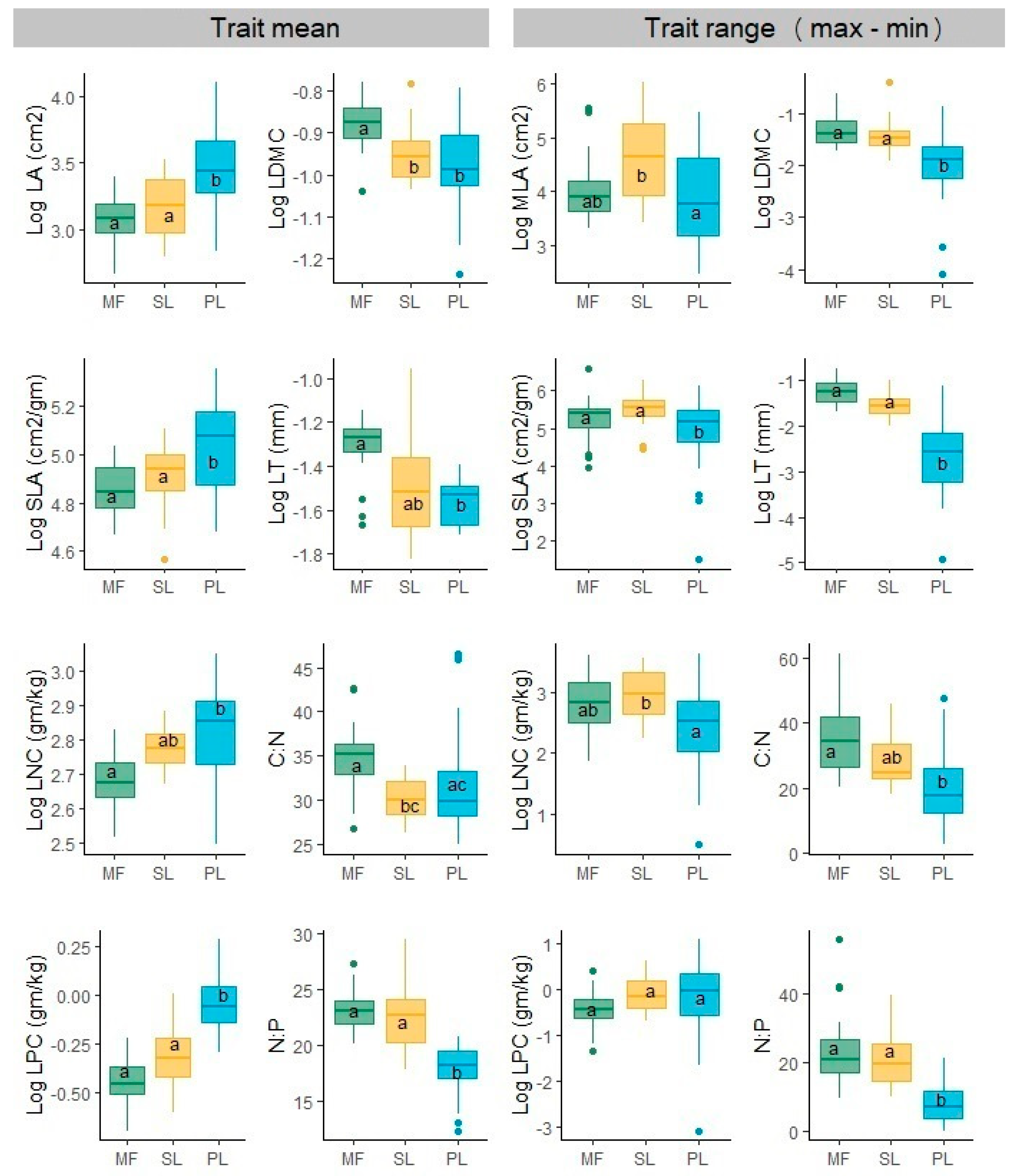
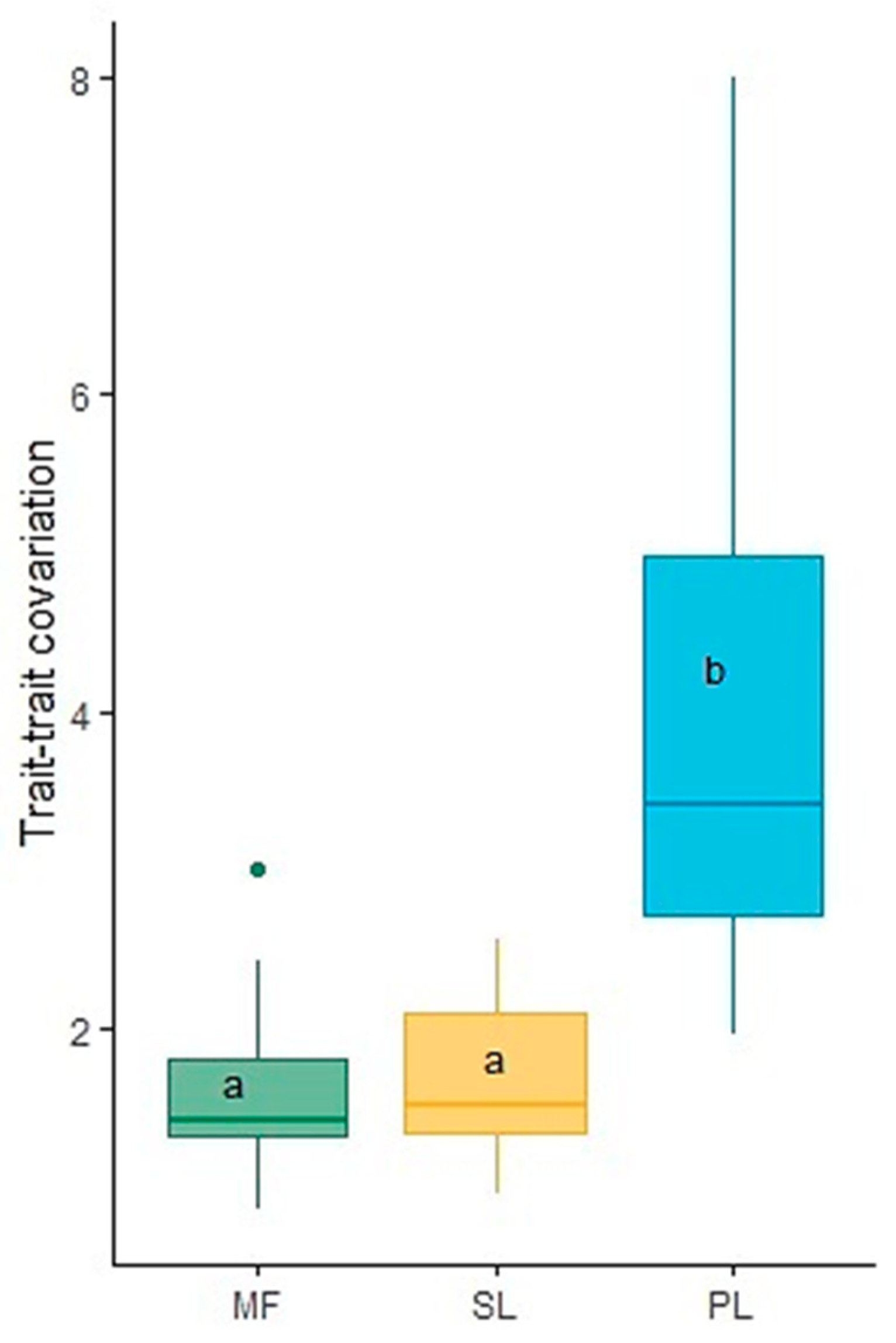
3.1. Community-Level Trait Mean, Range, and Trait–Trait Covariation Vary among Intact Mature Forest versus Post-Clearcut Secondary Forests

Community-weighted trait means differed markedly among forest communities (Figure 3; Supporting Information, Section S4). Plantations had, on average, higher leaf area, specific leaf area, and leaf nitrogen and phosphorus concentrations but lower leaf thickness, leaf dry matter content, C:N, and N:P than the shrubland or mature forest (all p-values < 0.01, Supporting Information, Section S4), confirming the dominance of resource acquisition strategy in the post-disturbance forest and resource conservation strategy in the mature forest. However, community-level trait ranges for most traits, except leaf phosphorus concentration (p = 0.106), was substantially narrower for plantation than shrubland or mature forest (Figure 3, Supporting Information, Section S4).

Similarly, plot-level trait–trait covariation was significantly higher in plantation than shrubland or mature forest (F_2,69 = 37.25; p < 0.001; Figure 4). While the differences in trait means for mature forest versus shrubland were somewhat apparent, those differences were negligible in their trait ranges.

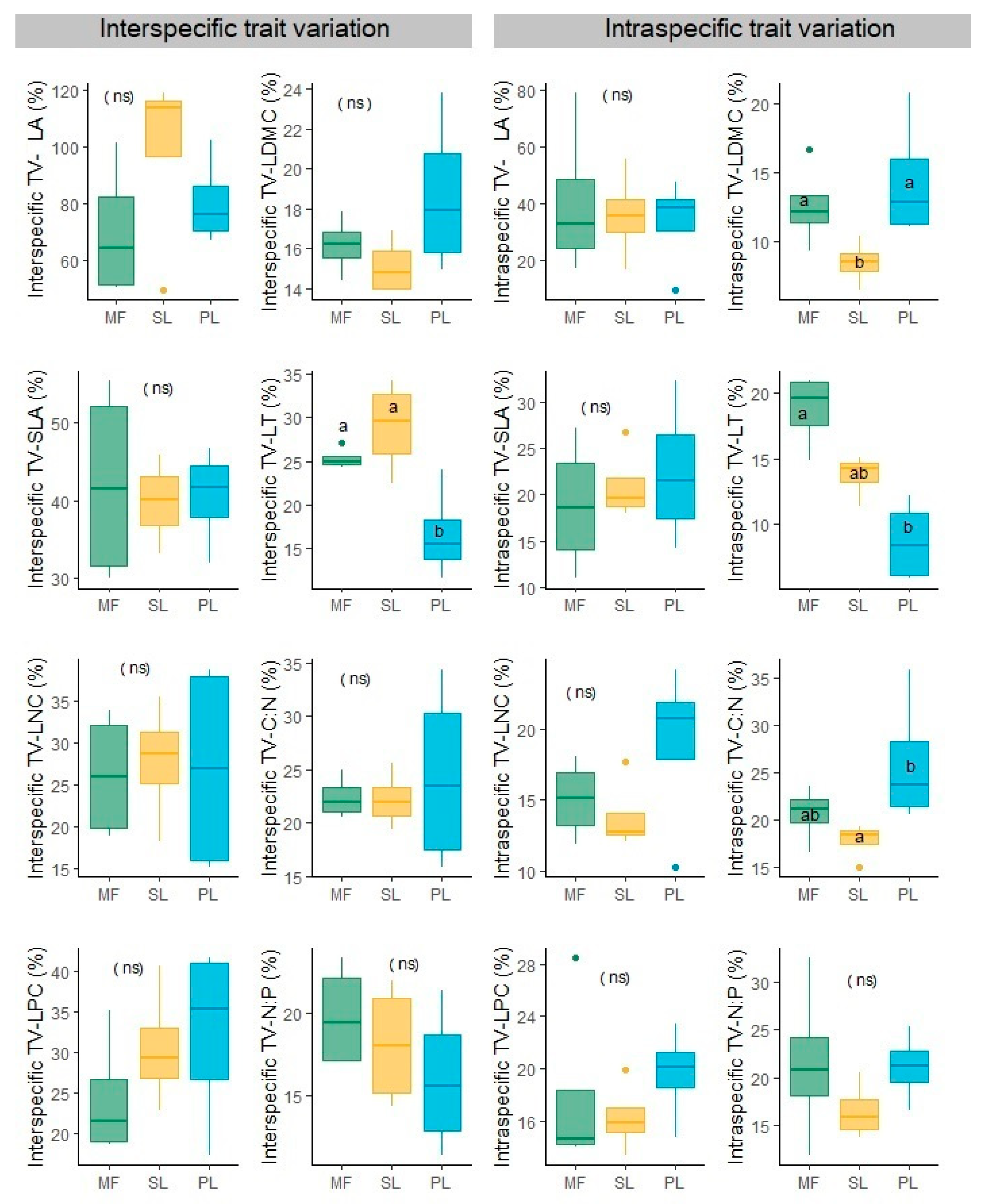
3.2. Community-Level Inter and Intraspecific Trait Variations Vary among Intact Mature Forest versus Post-Clearcut Secondary Forests

Multivariate inter and intraspecific trait variations across forest communities accounted for 67.8% and 32.2% of the variance, respectively. Such a pattern of inter- versus intraspecific trait variation held for individual traits (

Table 1. Patterns of interspecific versus intraspecific trait variations in the studied traits.

Traits	Interspecific Trait Variation (%)	Intraspecific Trait Variation (%)
LA	68.3	31.7
SLA	68.3	31.7
LDMC	60.5	39.5
LT	61.6	38.4
LNC	69.6	30.4
LPC	62	38
C:N	47.5	52.5
N:P	34.2	65.8

). However, mature forests and shrublands had slightly higher interspecific trait variations in leaf thickness (Kruskal–Wallis chi-squared_df=2 = 6.73; N = 12, p = 0.03) than in the plantation (Figure 5; Supporting Information, Section S5). In contrast, the plantation had slightly higher intraspecific trait variations in leaf dry matter content (KW chi-squared_df=2 = 6.58; N = 12; p = 0.03) and leaf C:N (KW chi-squared_df=2 = 6.03; N = 12; p < 0.05) than in shrublands (Figure 5). Compared to plantation or shrubland, the intraspecific trait variation in leaf thickness was also significantly higher at mature forests (KW chi-squared_df=2 = 8.65; N = 12; p = 0.01). While the differences in trait mean among mature forest and shrublands were somewhat apparent, those differences were negligible in their trait variations.

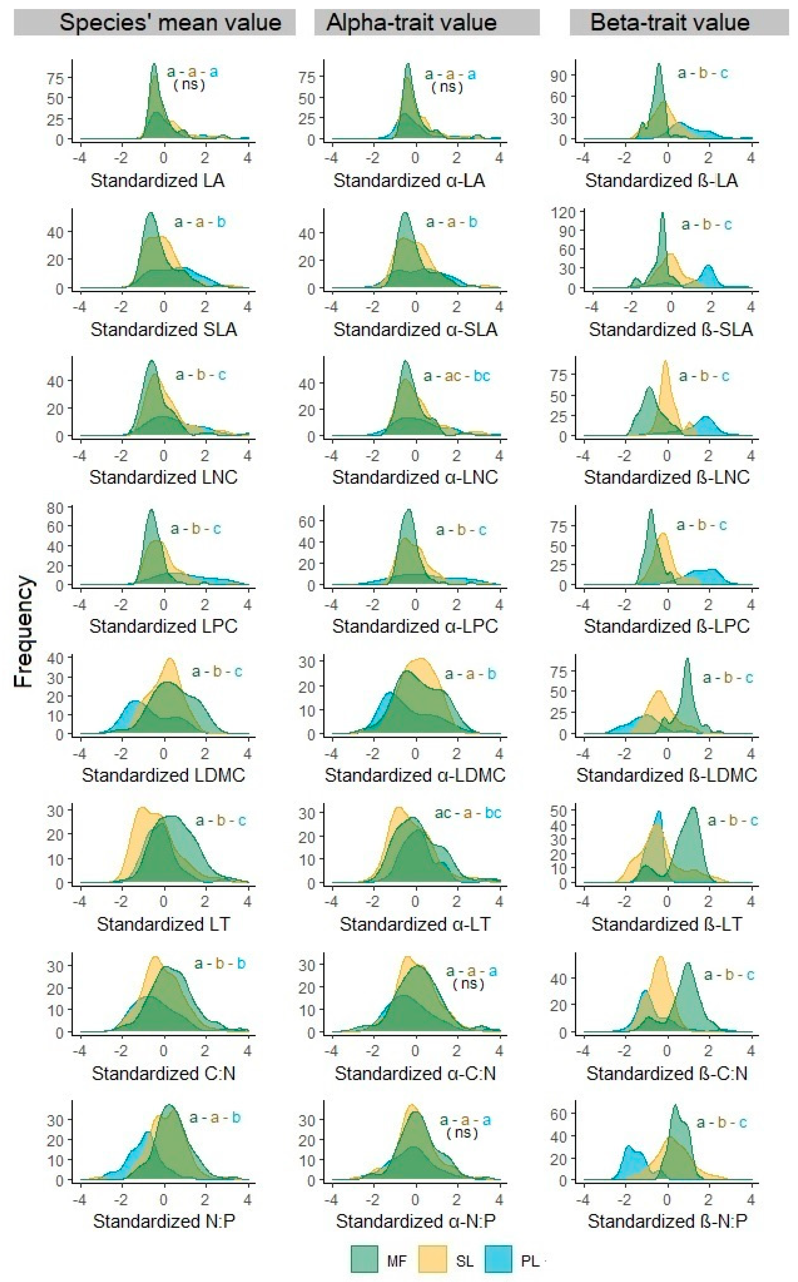
3.3. Species-Level Trait Mean, Alpha-Trait and Beta-Trait, and Niche-Breadth Vary among Intact Mature Forests versus Post-Clearcut Secondary Forests

The empirical distribution of species’ trait mean, alpha-trait and beta-trait values differed markedly among forest communities (Figure 6; Supporting Information, Section S6). More specifically, the frequency of species with higher mean trait values for resource acquisitive traits (SLA, LNC, and LPC) was substantially higher at plantations than the shrubland or mature forest (Supporting Information, Section S7). By contrast, the frequency of species with higher mean trait values for resource conservative traits (LT, LDMC, C:N, and N:P) was substantially higher at mature forests than at the plantation. However, when looking into the component of species’ beta-trait value that is reflective of environmental filtering, the overall pattern of resource acquisitive versus conservative traits was similar, but the differences among forest communities were more striking (Supporting Information, Section S7). By contrast, when looking into the component of species’ alpha-trait value reflective of competition, the overall pattern blurred, and the differences among forest communities were unclear.

Consistent across traits (except for LA and LPC), the frequency of species having higher niche breadth was substantially higher at mature forests than at the plantation, confirming that a less stressful environment provides greater niche breadth (Figure 7; Supporting Information, Sections S8 and S9). Conversely, the higher frequency of species with lower niche breadth may point towards stringent environmental filtering at the plantation. While the differences in species niche breadth among mature forest versus plantation were somewhat apparent, those differences were negligible for mature forest versus shrublands.

4. Discussion

Our study demonstrates the shifting importance of site condition-mediated environmental filtering and inter and intraspecific competition-mediated biotic filtering from undisturbed mature forests to post-disturbance secondary forests. Our study also validates a commonly held assumption that ecological processes leave their signatures on plant functional traits; hence, analysis of community and species-level trait structures can help disentangle processes from a pattern. These results, as discussed below, will contribute towards an improved understanding of forest biodiversity maintenance processes and, thereby, help conserve and manage forested ecosystems effectively.

4.1. Shifting Ecological Strategies along a Disturbance Gradient

Consistent with Garnier et al. [64] and many other earlier studies [65,66,67,68], our results indicate that high LA, SLA, LNC, and LNP are the hallmarks of plantation with a severe disturbance history, while intact mature forests communities were characterized by high LT, LDMC, C:N, and N:P (Figure 3 and Figure 6). This means that plantations are represented by species with faster growth, thinner and softer leaves with limited nutrients, while mature forests are marked by the slower growth rate, thicker leaves, and more nutrients in leaves. A fast-growing species acquires and consumes resources instead of preserving them and thus can quickly occupy the vacant niche in a post-disturbance early successional community. A slow-growing species in a mature forest, by contrast, conserves resources and thus survives along with coexisting species through competition [26]. Hence, the shifting importance of resource acquisition to conservation strategy for disturbed versus undisturbed forests is consistent with the concept of the leaf economic spectrum [69]. Additionally, our results of higher leaf nitrogen to phosphorus ratio (N:P) from disturbed to undisturbed control sites may indicate phosphorus limitation in intact primary forests [70]. Nevertheless, community functional structures of shrublands seem to resemble those of mature forests, suggesting their efficient recovery following clearcutting through successional processes.

4.2. Shifting Importance of Assembly Processes along a Disturbance Gradient

Our community-level analyses revealed a relatively narrow trait range and a more substantial degree of trait integration at the plantation, suggesting stringent environmental filtering in the post-clearcut plantation. Conversely, a comprehensive trait range coupled with a weaker trait integration may mean a slightly softer degree of environmental filtering in the mature forest (control) or post-clearcut shrubland. In complementary species-level analyses, we found the consistent dominance of species with broader niche breadths and lower beta-trait values for resource-acquisitive traits in mature forests; both indicate weaker environmental filtering. Hence, by taking the results of community and species-level analyses together, it is very likely that the strength of abiotic filtering increases with increasing disturbance.

Mechanistically, resource-conservative traits’ values (mean and ranges) are positively associated with site productivity, while trait ranges decrease with soil disturbance. Hence, disturbance-mediated reduced site productivity (Figure 2) may contribute towards the reduced values of LDMC, LT, C:N, and N:P in plantations (Figure 3). Alternatively, increased soil disturbance attributed to clearcutting and soil preparation (Figure 2) may filter out resource-conservative species and allow species with only resource acquisitive traits. That being said, environmental filtering can be stabilizing (i.e., unimodal trait response along environmental gradient), disruptive (i.e., bimodal trait response), or directional (i.e., linearly increasing or decreasing trait response) [71]. Results of our species’ niche breaths indicate that most of the traits showed a bimodal response (Figure 7), suggesting the play of disruptive environmental filtering structuring subtropical forest communities.

Meanwhile, species trait variations reflective of biotic filtering varied somewhat weakly among post-clearcut secondary forests versus intact mature forests. Yet, interspecific variation in leaf thickness was strikingly higher in the mature forest than in a plantation. In contrast, intraspecific variations in LDMC and C:N were higher in the plantation. It is, thus, likely that interspecific competition is somewhat essential for structuring mature forests and shrubland communities, while intraspecific competition may be necessary for structuring plantation communities.

Nevertheless, inter and intraspecific trait variation can be driven by multiple factors such as taxonomic differences in phylogeny, genetic differences, and phenotypic plasticity [72]. The trait variation among individuals of the same species (i.e., intraspecific trait variation) or different species (interspecific trait variation) provides some individuals within populations or some species with specialized behavior or form that could provide advantages when obtaining resources or competing with co-occurring individuals and species [73,74]. However, constrained by trait plasticity or heritable trait difference [75], both environmental filtering and biotic competition will constrain or enhance inter- as well as intra-specific trait variation [76], which make it hard to detect the association among environmental factors and trait variation, or disturbance effects on the patterns and determinants of trait variation. Additionally, due to logistical constraints, we could sample intraspecific trait variation at the site level instead of plot-level and focus on only three individuals from a species instead of all individuals, potentially making it difficult to detect the localized effects of disturbance on trait variation patterns, unlike a clear signal on trait mean, range of covariation. Sampling species traits from all individuals at the plot level and along a disturbance gradient may be a worthy topic to explore in the future.

4.3. Implications for Management

The most notorious factor contributing to the ongoing loss of biodiversity and the concomitant loss of ecosystem functions and services is anthropogenic habitat modification [77,78,79,80], and the most dominant form of habitat modification is forest conversion. According to the latest assessment by the Food and Agricultural Organization of the United Nations [81], the area of relatively intact mature forests has been shrinking at about eight million hectares per year between 1990 and 2020. Clearcutting is a reasonably common forestry practice in the subtropics [8]; forest managers are tasked with raising and managing post-clearcut secondary forests that can structurally and functionally resemble a pre-disturbance intact mature forest. Therefore, a detailed understanding of biodiversity maintenance processes in natural versus human-modified habitats is crucial for forest conservation planning. To that end, our study suggests that the relative importance of external versus internal filters could vary among undisturbed versus post-disturbance secondary forests. More specifically, we show a clear dominance of resource acquisition strategy in plantation versus resource conservation strategy in the mature forests. Those plantations had significantly lower trait ranges than mature forest or shrubland, suggesting the play of stringent environmental filtering in the plantation. However, intraspecific trait variation in some traits was high in plantation communities, while interspecific trait variation in other traits was high in intact mature forests, suggesting the importance of intra- versus inter-specific competition in plantation versus mature forests. Such shifting importance of site condition-mediated environmental filtering and intraspecific competition-mediated biotic filtering in the plantation to interspecific competition-mediated biotic filtering in the intact mature forests and shrublands can help inform forest management. For instance, plantation forestry can benefit from thinning operations to reduce intraspecific competition and minimize soil disturbance to improve site productivity and diversity.

References

1. Cornwell, W.K.; Ackerly, D.D. Community assembly and shifts in plant trait distributions across an environmental gradient in coastal California. Ecol. Monogr. 2009, 79, 109–126. [Google Scholar] [CrossRef] [Green Version]
2. Spasojevic, M.J.; Suding, K.N. Inferring community assembly mechanisms from functional diversity patterns: The importance of multiple assembly processes. J. Ecol. 2012, 100, 652–661. [Google Scholar] [CrossRef]
3. Kraft, N.J.B.; Adler, P.B.; Godoy, O.; James, E.C.; Fuller, S.; Levine, J.M. Community assembly, coexistence and the environmental filtering metaphor. Funct. Ecol. 2015, 29, 592–599. [Google Scholar] [CrossRef]
4. Ottaviani, G.; Tsakalos, J.L.; Keppel, G.; Mucina, L. Quantifying the effects of ecological constraints on trait expression using novel trait-gradient analysis parameters. Ecol. Evol. 2018, 8, 435–440. [Google Scholar] [CrossRef] [PubMed] [Green Version]
5. Cadotte, M.W.; Tucker, C.M. Should Environmental Filtering be Abandoned? Trends Ecol. Evol. 2017, 32, 429–437. [Google Scholar] [CrossRef]
6. Violle, C.; Enquist, B.J.; Mcgill, B.J.; Jiang, L.; Albert, C.H.; Hulshof, C.; Jung, V.; Messier, J. The return of the variance: Intraspecific variability in community ecology. Trends Ecol. Evol. 2012, 27, 244–252. [Google Scholar] [CrossRef]
7. Han, X.; Huang, J.; Yao, J.; Xu, Y.; Ding, Y.; Zang, R. Effects of logging on the ecological strategy spectrum of a tropical montane rain forest. Ecol. Indic. 2021, 128, 107812. [Google Scholar] [CrossRef]
8. Chazdon, R.L. Second Growth: The Promise of Tropical Forest Regeneration in an Age of Deforestation; University of Chicago Press: Chicago, IL, USA, 2014. [Google Scholar]
9. Ding, Y.; Zang, R.; Lu, X.; Huang, J. The impacts of selective logging and clear-cutting on woody plant diversity after 40 years of natural recovery in a tropical montane rain forest, south China. Sci. Total Environ. 2017, 579, 1683–1691. [Google Scholar] [CrossRef]
10. Chazdon, R.L. Tropical forest recovery: Legacies of human impact and natural disturbances. Perspect. Plant Ecol. Evol. Syst. 2003, 6, 51–71. [Google Scholar] [CrossRef] [Green Version]
11. Yan, E.-R.; Wang, X.-H.; Huang, J.-J. Shifts in plant nutrient use strategies under secondary forest succession. Plant Soil 2006, 289, 187–197. [Google Scholar] [CrossRef]
12. Wang, X.-H.; Kent, M.; Fang, X.-F. Evergreen broad-leaved forest in Eastern China: Its ecology and conservation and the importance of resprouting in forest restoration. For. Ecol. Manag. 2007, 245, 76–87. [Google Scholar] [CrossRef]
13. Guariguata, M.R.; Ostertag, R. Neotropical secondary forest succession: Changes in structural and functional characteristics. For. Ecol. Manag. 2001, 148, 185–206. [Google Scholar] [CrossRef]
14. Biswas, S.R.; Mallik, A.U. Disturbance effects on species diversity and functional diversity in riparian and upland plant communities. Ecology 2010, 91, 28–35. [Google Scholar] [CrossRef] [PubMed]
15. Clements, F.E. Plant Succession: An Analysis of the Development of Vegetation; Carnegie Institution of Washington: Washington, DC, USA, 1916; Volume 242. [Google Scholar]
16. Odum, E.P. The Strategy of Ecosystem Development. Science 1969, 164, 262–270. [Google Scholar] [CrossRef] [PubMed] [Green Version]
17. Ackerly, D.D.; Cornwell, W.K. A trait-based approach to community assembly: Partitioning of species trait values into within- and among-community components. Ecol. Lett. 2007, 10, 135–145. [Google Scholar] [CrossRef] [PubMed]
18. Weiher, E.; Keddy, P.A. Assembly Rules, Null Models, and Trait Dispersion: New Questions from Old Patterns. Oikos 1995, 74, 159–164. [Google Scholar] [CrossRef] [Green Version]
19. Cornwell, W.K.; Schwilk, D.W.; Ackerly, D.D. A trait-based test for habitat filtering: Convex hull volume. Ecology 2006, 87, 1465–1471. [Google Scholar] [CrossRef]
20. Dwyer, J.M.; Laughlin, D.C. Constraints on trait combinations explain climatic drivers of biodiversity: The importance of trait covariance in community assembly. Ecol. Lett. 2017, 20, 872–882. [Google Scholar] [CrossRef]
21. He, D.; Biswas, S.R.; Xu, M.S.; Yang, T.H.; You, W.H.; Yan, E.R. The importance of intraspecific trait variability in promoting functional niche dimensionality. Ecography 2021, 44, 380–390. [Google Scholar] [CrossRef]
22. MacArthur, R.; Levins, R. The limiting similarity, convergence, and divergence of coexisting species. Am. Nat. 1967, 101, 377–385. [Google Scholar] [CrossRef]
23. Spasojevic, M.J.; Turner, B.L.; Myers, J.A. When does intraspecific trait variation contribute to functional beta-diversity? J. Ecol. 2016, 104, 487–496. [Google Scholar] [CrossRef] [Green Version]
24. Gross, N.; Kunstler, G.; Liancourt, P.; De Bello, F.; Suding, K.N.; Lavorel, S. Linking individual response to biotic interactions with community structure: A trait-based framework. Funct. Ecol. 2009, 23, 1167–1178. [Google Scholar] [CrossRef]
25. Westerband, A.C.; Funk, J.L.; Barton, K.E. Intraspecific trait variation in plants: A renewed focus on its role in ecological processes. Ann. Bot. 2021, 127, 397–410. [Google Scholar] [CrossRef] [PubMed]
26. Yao, L.; Ding, Y.; Yao, L.; Ai, X.; Zang, R. Trait Gradient Analysis for Evergreen and Deciduous Species in a Subtropical Forest. Forests 2020, 11, 364. [Google Scholar] [CrossRef] [Green Version]
27. Xiang, J. Effects of Forest Conversion on Spatial Aotocorrelation in Plant Species and Functional Diversity in Tiantong National Forest Park. Master’s Thesis, East China Normal University, Shanghai, China, 2021. [Google Scholar]
28. Lu, H.P.; Wagner, H.H.; Chen, X.Y. A contribution diversity approach to evaluate species diversity. Basic Appl. Ecol. 2007, 8, 1–12. [Google Scholar] [CrossRef]
29. Da, L.; Yang, Y.; Song, Y. Poplation structure and regneration types of dominant speies in evergreen broadleaved forest in tiantong national forest park, Zhejiang province, eastern china. Acta Phytoecol. Sin. 2004, 28, 376–384. [Google Scholar]
30. Li, H. Scale-Dependent Effects of Forest Conversion on Species and Functional Diversity in Zhejiang Tiantong National Forest Park. Master’s Thesis, East China Normal University, Shanghai, China, 2021. [Google Scholar]
31. Yang, Q.; Ma, Z.; Xie, Y.; Zhang, Z.; Wang, Z.; Liu, H.; Li, P.; Zhang, N.; Wang, D.; Yang, H.; et al. Community structure and species composition of an evergreen broad-leaved forest in Tiantong’s 20 ha dynamic plot, Zhejiang Province, eastern China. Biodivers. Sci. 2011, 19, 215–223. [Google Scholar]
32. Zhejiang Provincial Bureau of Statistics. Zhejiang Statistical Yearbook; Zhejiang Provincial Bureau of Statistics: Hangzhou, China, 2020.
33. Ding, S.; Song, Y. Study on the synecological characteristics of the early successional stage of an evergreen broadleaved forest on Tiantong National Forest Park, Zhejiang province. Acta Phytoecol. Sin. 1999, 23, 97–107. [Google Scholar]
34. Adler, P.B.; Salguero-Gomez, R.; Compagnoni, A.; Hsu, J.S.; Ray-Mukherjee, J.; Mbeau-Ache, C.; Franco, M. Functional traits explain variation in plant life history strategies. Proc. Natl. Acad. Sci. USA 2014, 111, 740–745. [Google Scholar] [CrossRef] [Green Version]
35. Reich, P.B.; Walters, M.B.; Ellsworth, D.S. From tropics to tundra: Global convergence in plant functioning. Proc. Natl. Acad. Sci. USA 1997, 94, 13730–13734. [Google Scholar] [CrossRef] [Green Version]
36. Garnier, E.; Cortez, J.; Billes, G.; Navas, M.L.; Roumet, C.; Debussche, M.; Laurent, G.; Blanchard, A.; Aubry, D.; Bellmann, A.; et al. Plant functional markers capture ecosystem properties during secondary succession. Ecology 2004, 85, 2630–2637. [Google Scholar] [CrossRef]
37. Gratani, L.; Varone, L.; Crescente, M.F.; Catoni, R.; Ricotta, C.; Puglielli, G. Leaf thickness and density drive the responsiveness of photosynthesis to air temperature in Mediterranean species according to their leaf habitus. J. Arid. Environ. 2018, 150, 9–14. [Google Scholar] [CrossRef]
38. Bakker, M.A.; Carreno-Rocabado, G.; Poorter, L. Leaf economics traits predict litter decomposition of tropical plants and differ among land use types. Funct. Ecol. 2011, 25, 473–483. [Google Scholar] [CrossRef]
39. Carreno-Rocabado, G.; Pena-Claros, M.; Bongers, F.; Diaz, S.; Quetier, F.; Chuvina, J.; Poorter, L. Land-use intensification effects on functional properties in tropical plant communities. Ecol. Appl. 2016, 26, 174–189. [Google Scholar] [CrossRef] [PubMed] [Green Version]
40. Pauli, D.; White, J.W.; Andrade-Sanchez, P.; Conley, M.M.; Heun, J.; Thorp, K.R.; French, A.N.; Hunsaker, D.J.; Carmo-Silva, E.; Wang, G.; et al. Investigation of the Influence of Leaf Thickness on Canopy Reflectance and Physiological Traits in Upland and Pima Cotton Populations. Front. Plant Sci. 2017, 8, 1405. [Google Scholar] [CrossRef] [PubMed] [Green Version]
41. Gillison, A.N. Plant functional indicators of vegetation response to climate change, past present and future: I. Trends, emerging hypotheses and plant functional modality. Flora 2019, 254, 12–30. [Google Scholar] [CrossRef]
42. Hunt, E.R.; Weber, J.A.; Gates, D.M. Effects of Nitrate Application on Amaranthus powellii Wats. III. Optimal Allocation of Leaf Nitrogen for Photosynthesis and Stomatal Conductance. Plant Physiol. 1985, 79, 619–624. [Google Scholar] [CrossRef]
43. Reich, P.B.; Oleksyn, J. Global patterns of plant leaf N and P in relation to temperature and latitude. Proc. Natl. Acad. Sci. USA 2004, 101, 11001–11006. [Google Scholar] [CrossRef] [Green Version]
44. Zhang, J.; He, N.; Liu, C.; Xu, L.; Chen, Z.; Li, Y.; Wang, R.; Yu, G.; Sun, W.; Xiao, C.; et al. Variation and evolution of C:N ratio among different organs enable plants to adapt to N-limited environments. Glob. Chang. Biol. 2020, 26, 2534–2543. [Google Scholar] [CrossRef]
45. Güsewell, S. N:P ratios in terrestrial plants: Variation and functional significance. New Phytol. 2004, 164, 243–266. [Google Scholar] [CrossRef]
46. Chen, X.; Chen, H.Y.H. Plant mixture balances terrestrial ecosystem C:N:P stoichiometry. Nat. Commun. 2021, 12, 4562. [Google Scholar] [CrossRef] [PubMed]
47. Cornelissen, J.H.C.; Lavorel, S.; Garnier, E.; Díaz, S.; Buchmann, N.; Gurvich, D.E.; Reich, P.B.; Steege, H.T.; Morgan, H.D.; van der Heijden, M.G.A.; et al. A handbook of protocols for standardised and easy measurement of plant functional traits worldwide. Aust. J. Bot. 2003, 51, 335–380. [Google Scholar] [CrossRef] [Green Version]
48. Pérez-Harguindeguy, N.; Díaz, S.; Garnier, E.; Lavorel, S.; Poorter, H.; Jaureguiberry, P.; Bret-Harte, M.S.; Cornwell, W.K.; Craine, J.M.; Gurvich, D.E.; et al. New handbook for standardised measurement of plant functional traits worldwide. Aust. J. Bot. 2013, 61, 167–234. [Google Scholar] [CrossRef]
49. Licon, C. Proximate and Other Chemical Analyses. In Encyclopedia of Dairy Sciences, 3rd ed.; McSweeney, P.L.H., McNamara, J.P., Eds.; Academic Press: Oxford, MA, USA, 2022; pp. 521–529. [Google Scholar] [CrossRef]
50. Guo, H.-N.; Wang, L.-X.; Liu, H.-T. Potential mechanisms involving the immobilization of Cd, As and Cr during swine manure composting. Sci. Rep. 2020, 10, 16632. [Google Scholar] [CrossRef] [PubMed]
51. Nelson, D.W.; Sommers, L. A rapid and accurate procedure for estimation of organic carbon in soils. In Proceedings of the Indiana Academy of Science; Springer: Berlin/Heidelberg, Germany, 1974; pp. 456–462. [Google Scholar]
52. Widjaja, A.; Morris, R.J.; Levy, J.C.; Frayn, K.N.; Manley, S.E.; Turner, R.C. Within- and Between-Subject Variation in Commonly Measured Anthropometric and Biochemical Variables. Clin. Chem. 1999, 45, 561–566. [Google Scholar] [CrossRef] [PubMed]
53. Bivand, R.; Pebesma, E.; Gomez-Rubio, V. Applied Spatial Data Analysis with R, 2nd ed.; Springer: New York, NY, USA, 2013. [Google Scholar]
54. Pinheiro, J.; Bates, D.; DebRoy, S.; Sarkar, D.; R Core Team. nlme: Linear and Nonlinear Mixed Effects Models, R package version 3.1-153; 2021. Available online: https://cran.r-project.org/web/packages/nlme/nlme.pdf (accessed on 25 February 2022).
55. Lenth, R.V. Least-Squares Means: The R Package lsmeans. J. Stat. Softw. 2016, 69, 1–33. [Google Scholar] [CrossRef] [Green Version]
56. Fox, J.; Weisberg, S. An R Companion to Applied Regression, 3rd ed.; Sage Publications: Thousand Oaks, CA, USA, 2019. [Google Scholar]
57. Kassambara, A. rstatix: Pipe-Friendly Framework for Basic Statistical Tests, R package version 0.6.0.; 2020. Available online: https://cran.r-project.org/web/packages/rstatix/index.html (accessed on 25 February 2022).
58. Dunn, O.J. Multiple comparisons among means. JASA 1961, 56, 54–64. [Google Scholar] [CrossRef]
59. Dinno, A. Dunn. Test: Dunn’s Test of Multiple Comparisons Using Rank Sums, R package version 1.3.5.; 2017. Available online: https://cran.r-project.org/web/packages/dunn.test/dunn.test.pdf (accessed on 25 February 2022).
60. R Core Team. R: A Language and Environment for Statistical Computing; Foundation for Statistical Computing: Vienna, Austria, 2020. [Google Scholar]
61. Wickham, H. ggplot2: Elegant Graphics for Data Analysis; Springer: New York, NY, USA, 2016. [Google Scholar]
62. Bryan, J. gapminder: Data from Gapminder, R package version 0.3.0.; 2017. Available online: https://cran.r-project.org/web/packages/gapminder/gapminder.pdf (accessed on 25 February 2022).
63. Kassambara, A. ggpubr: ‘ggplot2’ Based Publication Ready Plots, R package version 0.4.0.; 2020. Available online: https://cran.r-project.org/web/packages/ggpubr/index.html (accessed on 25 February 2022).
64. Garnier, E.; Lavorel, S.; Ansquer, P.; Castro, H.; Cruz, P.; Dolezal, J.; Eriksson, O.; Fortunel, C.; Freitas, H.; Golodets, C.; et al. Assessing the Effects of Land-use Change on Plant Traits, Communities and Ecosystem Functioning in Grasslands: A Standardized Methodology and Lessons from an Application to 11 European Sites. Ann. Bot. 2006, 99, 967–985. [Google Scholar] [CrossRef] [Green Version]
65. Poorter, L.; Rozendaal, D.M.A.; Bongers, F.; De Almeida-Cortez, J.S.; Almeyda Zambrano, A.M.; Álvarez, F.S.; Andrade, J.L.; Villa, L.F.A.; Balvanera, P.; Becknell, J.M.; et al. Wet and dry tropical forests show opposite successional pathways in wood density but converge over time. Nat. Ecol. Evol. 2019, 3, 928–934. [Google Scholar] [CrossRef]
66. Lohbeck, M.; Poorter, L.; Lebrija-Trejos, E.; Martínez-Ramos, M.; Meave, J.A.; Paz, H.; Pérez-García, E.A.; Romero-Pérez, I.E.; Tauro, A.; Bongers, F. Successional changes in functional composition contrast for dry and wet tropical forest. Ecology 2013, 94, 1211–1216. [Google Scholar] [CrossRef]
67. Aiba, M.; Kurokawa, H.; Onoda, Y.; Oguro, M.; Nakashizuka, T.; Masaki, T. Context-dependent changes in the functional composition of tree communities along successional gradients after land-use change. J. Ecol. 2016, 104, 1347–1356. [Google Scholar] [CrossRef] [Green Version]
68. Kang, M.; Chang, S.X.; Yan, E.-R.; Wang, X.-H. Trait variability differs between leaf and wood tissues across ecological scales in subtropical forests. J. Veg. Sci. 2014, 25, 703–714. [Google Scholar] [CrossRef]
69. Wright, I.J.; Reich, P.B.; Westoby, M.; Ackerly, D.D.; Baruch, Z.; Bongers, F.; Cavender-Bares, J.; Chapin, T.; Cornelissen, J.H.C.; Diemer, M.; et al. The worldwide leaf economics spectrum. Nature 2004, 428, 821–827. [Google Scholar] [CrossRef] [PubMed]
70. Yan, E.-R.; Zhou, W.; Wang, X.-H. N:P stoichiometry in secondary succession in evergreen broad-leaved forest, Tiantong, East China. Chin. J. Plant Ecol. 2008, 32, 13–22. [Google Scholar] [CrossRef]
71. Munoz, F.; Grenié, M.; Denelle, P.; Taudière, A.; Laroche, F.; Tucker, C.; Violle, C. ecolottery: Simulating and assessing community assembly with environmental filtering and neutral dynamics in R. Methods Ecol. Evol. 2018, 9, 693–703. [Google Scholar] [CrossRef]
72. Hofhansl, F.; Chacon-Madrigal, E.; Brannstrom, A.; Dieckmann, U.; Franklin, O. Mechanisms driving plant functional trait variation in a tropical forest. Ecol. Evol. 2021, 11, 3856–3870. [Google Scholar] [CrossRef]
73. Bolnick, D.I.; Svanbäck, R.; Fordyce, J.A.; Yang, L.H.; Davis, J.M.; Hulsey, C.D.; Forister, M.L. The Ecology of Individuals: Incidence and Implications of Individual Specialization. Am. Nat. 2003, 161, 1–28. [Google Scholar] [CrossRef]
74. Araújo, M.S.; Bolnick, D.I.; Layman, C.A. The ecological causes of individual specialisation. Ecol. Lett. 2011, 14, 948–958. [Google Scholar] [CrossRef]
75. Carvajal, D.E.; Loayza, A.P.; Rios, R.S.; Delpiano, C.A.; Squeo, F.A. A hyper-arid environment shapes an inverse pattern of the fast-slow plant economics spectrum for above-, but not below-ground resource acquisition strategies. J. Ecol. 2019, 107, 1079–1092. [Google Scholar] [CrossRef]
76. Kuppler, J.; Albert, C.H.; Ames, G.M.; Armbruster, W.S.; Boenisch, G.; Boucher, F.C.; Campbell, D.R.; Carneiro, L.T.; Chacon-Madrigal, E.; Enquist, B.J.; et al. Global gradients in intraspecific variation in vegetative and floral traits are partially associated with climate and species richness. Glob. Ecol. Biogeogr. 2020, 29, 992–1007. [Google Scholar] [CrossRef]
77. Sala, O.E.; Chapin III, S.F.; Armesto, J.J.; Berlow, E.; Bloomfield, J.; Dirzo, R.; Huber-Sanwald, E.; Huenneke, L.F.; Jackson, R.B.; Kinzig, A.; et al. Global Biodiversity Scenarios for the Year 2100. Science 2000, 287, 1770–1774. [Google Scholar] [CrossRef] [PubMed]
78. Pereira, H.M.; Leadley, P.W.; Proença, V.; Alkemade, R.; Scharlemann, J.P.W.; Fernandez-Manjarrés, J.F.; Araújo, M.B.; Balvanera, P.; Biggs, R.; Cheung, W.W.L.; et al. Scenarios for Global Biodiversity in the 21st Century. Science 2010, 330, 1496–1501. [Google Scholar] [CrossRef] [PubMed] [Green Version]
79. Newbold, T.; Hudson, L.N.; Hill, S.L.L.; Contu, S.; Lysenko, I.; Senior, R.A.; Börger, L.; Bennett, D.J.; Choimes, A.; Collen, B.; et al. Global effects of land use on local terrestrial biodiversity. Nature 2015, 520, 45. [Google Scholar] [CrossRef] [PubMed] [Green Version]
80. Edwards, D.P.; Socolar, J.B.; Mills, S.C.; Burivalova, Z.; Koh, L.P.; Wilcove, D.S. Conservation of Tropical Forests in the Anthropocene. Curr. Biol. 2019, 29, R1008–R1020. [Google Scholar] [CrossRef]
81. FAO; UNEP. The State of the World’s Forests 2020. Forests, Biodiversity and People; FAO: Rome, Italy, 2020. [Google Scholar] [CrossRef]
Figure 1. Location of study sites with representative figures of control versus treatment (shrubland and plantation).
Forests 13 00672 g001
Figure 2. Summarized representation of site abiotic (soil moisture, organic matter depth, canopy exposure, and soil compaction) and biotic conditions (richness, number of individuals, and species composition) for control (mature forest, MF) versus treatment (shrubland, SL and plantation, PL). Within a figure, boxes marked with the same letter do not differ significantly at α = 0.05 as identified by Tukey’s HSD test.
Forests 13 00672 g002
Figure 3. Plot-level trait mean and trait ranges for control (mature forest = MF) versus treatment (shrubland = SL and plantation = PL). Within a figure, boxes marked with the same letter do not differ significantly at α = 0.05 as identified by Tukey’s HSD test.
Forests 13 00672 g003
Figure 4. Plot-level trait–trait covariation for control (mature forest = MF) versus treatment (shrubland = SL and plantation = PL). Within a figure, boxes marked with the same letter do not differ significantly at α = 0.05 as identified by Tukey’s HSD test.
Forests 13 00672 g004
Figure 5. Site-level inter and intraspecific trait variations for control (mature forest = MF) versus treatment (shrubland = SL and plantation = PL). Within a figure, boxes marked with the same letter do not differ significantly at α = 0.05 as identified by Tukey’s HSD test.
Forests 13 00672 g005
Figure 6. Frequency distributions of species-level trait mean, alpha-trait, and beta-trait values for control (mature forest = MF) versus treatment (shrubland = SL and plantation = PL). Letter colored in sea green, goldenrod, and deep sky blue within each figure represent MF, SL, and PL sequentially, and having the same letter within a color refers to a non-significant difference α = 0.05 as identified by Kolmogorov–Smirnov tests.
Forests 13 00672 g006
Figure 7. Frequency distributions of species-level niche breadths for control (mature forest = MF) versus treatment (shrubland = SL and plantation = PL). Letter colored in sea green, goldenrod, and deep sky blue within each figure represent MF, SL, and PL sequentially, and having the same letter within a color refers to a non-significant difference α = 0.05 as identified by Kolmogorov–Smirnov tests.
Forests 13 00672 g007