Article

Application of the Reformulated Gash Analytical Model for Rainfall Interception Loss to Unmanaged High-Density Coniferous Plantations Laden with Dead Branches

1
Kasuya Research Forest, Kyushu University, Fukuoka 811-2415, Japan
2
Key Laboratory of Agricultural Water Resources, Center for Agricultural Resources Research, Institute of Genetics and Developmental Biology, Chinese Academy of Sciences, Shijiazhuang 050021, China
3
Shiiba Research Forest, Kyushu University, Shiiba, Miyazaki 761-0312, Japan
4
Faculty of Agriculture, University of Miyazaki, Miyazaki 889-2192, Japan
5
Ecohydrology Research Institute, The University of Tokyo Forests, Graduate School of Agricultural and Life Sciences, The University of Tokyo, Seto, Aichi 489-0031, Japan
*
Author to whom correspondence should be addressed.
Forests 2022, 13(5), 657; https://doi.org/10.3390/f13050657
Submission received: 3 March 2022 / Revised: 4 April 2022 / Accepted: 21 April 2022 / Published: 23 April 2022
(This article belongs to the Section Forest Hydrology)

Abstract

:
Interception loss (IL) by the forest canopy removes a substantial quantity of rainwater within forested ecosystems. The large-scale unmanaged Japanese coniferous plantations with high stand density (SD) in Japan raise concerns about an additional increasing IL as a result of a new influential factor of dead branches under canopies. Thus, evaluating the usage of IL estimation models is vital to regulating the water and environment in such coniferous plantations. This study aimed to examine the applicability of the reformulated Gash analytical model (RGAM) to unmanaged coniferous plantations with high SD laden with dead branches. We established two plots (P1 and P2) laden with dead branches under the same SD of 2250 stems ha−1 but with different numbers of dead branches (56 vs. 47 branches per tree) in an unmanaged Japanese coniferous plantation. Results demonstrated that a large difference was found in canopy storage capacity (S) in P1 and P2 (3.94 vs. 3.25 mm), which was influenced by the different number of dead branches; therefore, the IL ratio to gross rainfall differed considerably (32.7% in P1 and 26.7% in P2) regardless of the SD being the same. The difference in S enables the RGAM to reflect the influence of dead branch structures on IL, leading to an acceptable RGAM performance for both P1 and P2 (“fair” IL relative errors: −20.2% vs. −16.1%) in the present study of unmanaged coniferous plantations with high SD laden with dead branches.

1. Introduction

The forest canopy is the first contact surface for rainwater. When gross rainfall (GR) encounters forest canopies, it is partitioned into net rainfall (throughfall (TF): the portion falling to the forest floor through the canopy; stemflow (SF): the portion draining through the canopy along the branches and stem surfaces) and rainfall loss (interception loss (IL): the portion evaporating back to the atmosphere). The IL from trees is a primary component of evapotranspiration [1,2,3] and exerts a strong influence on the forest water resources and the environment in forest ecosystems [4,5,6,7,8,9]. The IL as a proportion of GR (IL/GR, %) is as much as 30% in mature coniferous plantations and is strongly influenced by forest stand structure parameters, such as stand density (SD), and canopy structure factors (plant area index, PAI; canopy cover, c) [2,4,6,8,10,11]. Therefore, understanding the effect of forest stand structure on IL is essential to regulating the water and environment in forest ecosystems.
Numerous studies of IL have been conducted in diverse forest types worldwide (e.g., [5,9,12,13]). Previous studies of IL conducted in different forest types determined the influence of forest stand structure factors, such as SD [4,11], c [6], PAI [14], and water storage capacity on the tree surface (S, [15]). These findings demonstrate that factors influential on IL depend on tree traits and climate conditions. Thus, studies of IL for the same species with different forest stand structures under the same climate condition help to give a better understanding of the changes in IL due to changes in forest stand structures, which would contribute to the assessment of local water and environmental management in forest ecosystems [2,4,11,16,17].
In Japan, forested areas account for 67% of the total land area, with plantations constituting 41% of the forested area [18]. The dominant plantation species are Japanese cedar (Cryptomeria japonica D.Don) and Japanese cypress (Chamaecyparis obtusa Endl.) with a typical planting density of ≥2500 stems ha−1 [18]. Many plantations, however, have not been managed adequately because of the impacts of economic recession on forestry since the 1980s [19]. Unmanaged plantations, compared with managed plantations, generally feature high SD, high c, and sparse understory vegetation (Figure 1). In addition, unmanaged plantations with high SD have a complex stand structure, such as dead branches under canopies (see Figure 1b, [17,20,21]).
Nanko et al. [22] examined TF drop velocity in an unmanaged Japanese cypress plantation. The authors reported that some drips of TF had a lower velocity than expected probably due to the influences of dead branches around the stem as well as leaves on live branches on TF partitioning. Shinohara et al. [23] pruned some of the many dead branches under canopies in Japanese cypress plantations and observed that dead branches influence raindrop erosivity induced by TF. Jeong et al. [17] detected strong correlations between TF and dead branch structures (a negative relationship between TF and number of dead branches and a positive relationship between TF and vertical distance of dead branches; see Figure 6 of [17]). These findings imply that IL, which is the difference between GR and the sum of TF and SF, may differ between upper-canopy structure and under-canopy structure with dead branches. Thus, evaluation of the accuracy of IL estimation models is vital for their potential application to unmanaged coniferous plantations laden with dead branches.
Various IL estimation models have been developed [13]: empirical models (e.g., [24,25]) and physically based models, such as numerical models (e.g., [26,27]), analytical models (e.g., [28,29]), and stochastic models (e.g., [30]).
Komatsu et al. [11] targeted the dominant plantation species in Japan growing in similar climates for estimation of IL in response to forest management practices, such as thinning. The authors developed an empirical regression IL estimation model based on the relationship between IL/GR and SD using 46 data sets for two dominant plantation species in regions without heavy snowfall. The authors found that none of the other parameters (canopy height, species, and annual precipitation) improved the predictability of IL. Nagano et al. [31] included three additional data sets for sparse Japanese coniferous plantations (i.e., n = 49, SD range: 356 to 3864 stems ha−1 with a mean of 1506 stems ha−1). The equation is formulated as follows:
IL/GR = 0.290 {1 − exp (−0.00110 ∗ SD)} × 100
Komatsu et al. [11] reported that the estimation error of IL using Equation (1), i.e., the absolute value of ILmodeled/GRILmeasured/GR, was as small as 4%. Komatsu et al. [11] did not explicitly state that unmanaged plantations laden with dead branches were included in the 49 datasets. Moreover, no previous studies have examined the applicability of Equation (1) to unmanaged coniferous plantations laden with dead branches.
The Gash analytical model was originally developed as a physically based IL estimation model in 1979 [28]. It was modified due to its failure to estimate IL in sparse forests [29], which is generally called the reformulated Gash analytical model (hereafter RGAM). Among physically based IL estimation models, RGAM is the most commonly used IL estimation model for various forest types worldwide (111 previous studies reviewed by Muzylo et al. [13]) because it requires relatively few parameters and variables that can be derived from observation data of forest stand structure, rainfall partitioning (RP), and meteorology [13]. The RGAM has been applied to unmanaged Japanese coniferous plantations before thinning [1] and after thinning [6], which showed that the RGAM is sufficiently robust and reliable for the estimation of IL for unmanaged Japanese coniferous plantations regardless of thinning practice. Although the presence of dead branches is known as the typical under-canopy characteristic in unmanaged Japanese coniferous plantations [20], the characteristics of dead branch structures (e.g., the number of dead branches [17,21]) has been poorly studied. Moreover, to the authors’ knowledge, no study has attempted to apply the RGAM to unmanaged Japanese coniferous plantations with high SD laden with dead branches almost fully distributed on the stems, although some previous studies may have implicitly tested the applicability of the RGAM in high-density coniferous plantations probably with dead branches.
This study aimed to examine the applicability of the RGAM to unmanaged coniferous plantations with high SD laden with dead branches. To do this, (1) we applied the RGAM to two Japanese coniferous plantation plots with the same high SD laden with dead branches but with different numbers of dead branches; (2) we performed a sensitivity analysis to detect essential parameters for RGAM IL estimation; and (3) we assessed the applicability of the RGAM together with Equation (1) to such coniferous plantations.

2. Materials and Methods
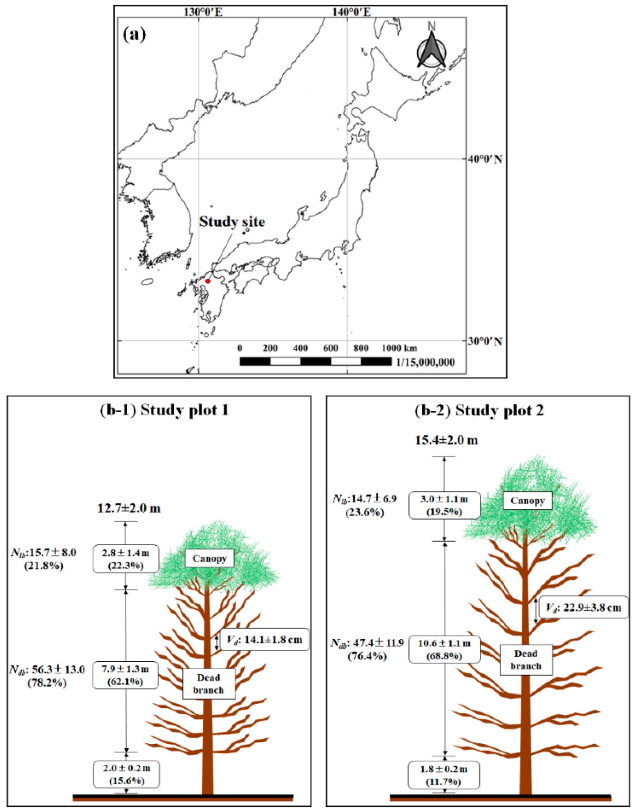
2.1. Study Site

The study site is located at the Takada experimental site of Kasuya Research Forest, Kyushu University, Fukuoka, Japan (33°37′58″ N, 130°31′48″ E, 100 m a.s.l.; Figure 2a). The study site is covered with Japanese cypress (Chamaecyparis obtusa Endl.) trees planted in 1985. The plantation has not been managed. The mean annual temperature and mean annual precipitation are 17.2 ± 0.5 (S.D.) °C and 1649.0 ± 337.6 (S.D.) mm, respectively, based on the Fukuoka meteorological observatory’s data for 1986−2017 measured at the nearest long-term meteorological station. The rainy and snowy seasons are from June to September and December to February, respectively [23].
Two 20 m × 10 m plots (hereafter P1 and P2, respectively) were established at the study site. P1 and P2 each contained 50 trees (i.e., 2500 stems ha−1), among which five standing trees were dead in each plot (i.e., in the process of self-thinning). Jeong and Otsuki [21] reported that the stand-scale SF/GR can be overestimated when standing-dead trees are considered alive and included for the calculation of the stand-scale SF/GR. The authors suggested that the stand-scale SF/GR would be reliably estimated with only standing-live trees, and the standing-dead trees should not be included in standing trees for stand-scale SF/GR estimation. Thus, the standing-dead trees were excluded from the SD calculation (i.e., 45 trees in each plot, equal to 2250 stems ha−1) to avoid errors in IL estimation through SF [21]. The plot slopes were relatively steep (26°). The forest structure was categorized into (1) stand structure, (2) upper-canopy structure, and (3) under-canopy structure (i.e., dead branch structure) (Figure 2b and Table 1). Stand structures and under-canopy structures were statistically different, whereas no statistical difference in upper-canopy structures was observed (Table 1). Specifically, stand structure parameters (diameter at breast height (DBH), h, basal area (BA), and PAI) were larger in P2 than those in P1 (t-test, p < 0.001). For under-canopy structures (number of dead branches (Ndb) and vertical distance of dead branches (Vd)), Ndb in P1 was larger than that in P2, and Vd in P1 was shorter than that in P2 (t-test, p ≤ 0.001). Upper-canopy structure parameters (number of live branches (Nlb), crown length (CL), and crown projection area (CPA)) were almost identical between P1 and P2 (t-test, p > 0.05).

2.2. Measurement of Throughfall and Stemflow

TF was monitored using 30 storage-type TF rain collectors (210-mm-diameter funnel) in P1 and 28 counterparts in P2. The TF rain collectors were randomly arranged and maintained throughout the study period. Note that the relative standard errors of the mean stand-scale TF between the two plots, assessed using the following Student’s t-value analysis at the significance level of 0.05, were almost identical (5.0% vs. 5.4%, [17,32]).
ε = ( t 0.05 , n 1 × C V ) n
where ε is the error of the mean, t0.05,n−1 is the Student’s t-value, CV is the coefficient of variation, and n is the number of TF rain collectors.
Nine standing live trees were selected to measure SF according to the DBH classes in each plot. SF was collected using a hose, plastic seat, and silicon sealant at the height of 1.5 m, which drained into two 90 L connected bins to prevent overflow. The stand-scale SF (mm) was estimated with the following equation [16,17,21,33]:
S F = S F V i n t r e e × N a l l P A
where SFVi is the sum of the SF volume (L) of the observed trees, ntree and Nall are the number of observed trees (n = 9) and all standing-live trees (n = 45) in each plot, respectively, and PA is the plot area (200 m2).
TF and SF were collected on a weekly basis but on a day with no rain during the growing season from April to October 2017. The range of the periods was 5 to 9 days, with an average of 7 days, and thus we call the period “weekly” hereafter. We obtained 25 weekly RP data and used them for the analysis. IL was calculated as the difference between GR and the sum of TF and SF as follows:
I L = G R ( T F + S F )
More detailed descriptions of the study site and measurement of RP are reported in our previous study [17].
The growing season from April to October is coincident with the rainy season in this region. The precipitation at the Fukuoka meteorological observatory from April to October during 1986−2017 was 621.5−1879.0 mm with a mean of 1244.0 ± 300.1 (S.D.) mm, accounting for 75.4% of the mean annual precipitation. During the study period from April to October 2017, total GR was 1068.4 mm, which accounted for 85.9% of the mean precipitation for the same period, which implies that the measurement period was under the normal meteorological condition of this region. Two previous studies reported no relation between annual GR and IL/GR for Japanese coniferous plantations in Japan [11,16] and also support this assumption that our measurements for IL estimation could be representative of general meteorological conditions in this region.

2.3. Measurement of Meteorological Data

Meteorological conditions were measured on a 2 m tower installed in an opening 50 m from P1 and P2. Before measuring meteorological conditions in the opening, we removed all obstructions such as trees and shrubs within 45° around the 2 m tower for similar meteorological conditions to the above-canopy conditions. We continuously managed the opening area during the study period. GR was measured using a tipping bucket with a resolution of 0.2 mm (HOBO RG3-M rain gauge, Onset Computer, Bourne, MA, USA) with a data logger (HOBO Event, Onset Computer, Bourne, MA, USA). There were missing data for 1 week from the 0.2 mm rain gauge (GR0.2), which were substituted with data from a tipping bucket with a resolution of 0.5 mm (GR0.5) measured in the opening (Ota Keiki Seisakusho Co. Ltd., Tokyo, Japan) (GR0.5 = 1.00 × GR0.2; R2 > 0.97). Air temperature (T, °C) and relative humidity (RH, %) were measured with a temperature/humidity probe (S-THB-M002, Onset Computer, Bourne, MA, USA). The data were recorded at 10 min intervals with a data logger (HOBO U30 Weather Station; Onset Computer, Bourne, MA, USA). Solar radiation (Rs) was measured in an opening site approximately 1 km away from the study site using a solar radiometer (ML-020VM, EKO Instruments, Tokyo, Japan). Wind speed (WS) was measured at Fukuoka airport, located approximately 7 km southwest of the study site, by the Japan Meteorological Agency.

2.4. Application of RGAM

In the RGAM, GR is deemed to occur as a series of discrete events and is separately analyzed using the threshold gross rainfall (GR′) to determine whether the canopy is saturated or not. Based on the rainfall and canopy structure, GR′ was determined as follows:
G R = R ¯ E c ¯ s c l n ( 1 E c ¯ R ¯ )
S c = S c
where R ¯ is mean GR rate during the saturated canopy conditions (mm h−1), E ¯ is mean wet canopy evaporation rate under saturated canopy conditions per unit ground area (mm h−1), E c ¯ is mean wet canopy evaporation rate under saturated canopy conditions from the canopy covered area (mm h−1), S is canopy storage capacity (mm), and Sc is canopy storage capacity per canopy cover (mm). Based on the assumption of Gash [28], R ¯ and E c ¯ were calculated for all the hourly periods with GR greater than 0.5 mm h−1, which could represent the average rainfall and evaporation rates under saturated canopy conditions, respectively.
For a given rainfall event, the components of IL were calculated as follows:
I L = {   I L i n s u f ,    G R < G R I L s u f ,    G R G R
where ILinsuf is the interception (mm) during a small rainfall event that was insufficient to saturate the canopy and ILsuf is the interception (mm) during a large rainfall event that was sufficient to saturate the canopy.
ILinsuf was calculated as follows:
I L i n s u f = c   j = 1 m G R j
where m is the number of storms that are insufficient to saturate the canopy.
ILsuf consists of four IL components and was calculated as follows:
I L s u f = I L w + I L s + I L d + I L t
I L w = n c ( G R S c )
I L s = c E c ¯ R ¯   j = 1 n ( G R j G R )
I L d = n c S c
I L t = q S t + p t   j = 1 n q G R j ( G R j > P t )
P t = S t / p t
where ILw is IL for wetting the canopy (mm), n is the number of storms sufficient to saturate the canopy, ILs is IL for wet canopy evaporation during storms (mm), ILd is IL for wet canopy evaporation after storms cease (mm), ILt is IL for evaporation from trunks (mm) for q storms that saturate the trunks, q is the number of storms sufficient to saturate the trunks, St is the trunk storage capacity (mm), pt is the proportion of rainfall diverted to SF, nq is the number of storms insufficient to saturate the trunks, and Pt′ is the threshold gross rainfall sufficient to saturate trunks (mm).
For calculation of the wet canopy evaporation rate under saturation canopy condition Ec (mm per unit of covered area, and assumed to be equal for the whole plot area), the Penman–Monteith equation setting canopy resistance (rs) to zero was used as follows:
E c = ( Δ R n + ρ c p D r a ) / λ ( Δ + γ )
where Δ is the rate of change of saturated vapor pressure with temperature (Pa K−1), Rn is the net radiation on the canopy (W m−2), ρ is the density of dry air (kg m−3), cp is the specific heat of air at constant temperature (J kg−1 K−1), D is the vapor pressure deficit (Pa), ra is the aerodynamic resistance (s m−1), λ is the latent heat of vaporization of water (J kg−1), and γ is the psychometric constant (Pa K−1). Given that we did not measure net radiation, Rn was assumed to be 0.8 times Rs [4,8], where Rs is the incident solar radiation (W m−2).
The RGAM can be run both on an event basis (e.g., [6,8]) and on a daily basis assuming one storm per rain day [29]. In this study, the RGAM was run on an event basis. The drying time for canopy wetting in Japanese coniferous plantations was assumed to be 6−8 h in the humid temperate climate of Japan (e.g., [6,8,16]). Consequently, a rainfall event was classified as a separate event when the period without rainfall after its cessation exceeded 8 h. Among 25 weekly data sets, 6 data sets included a single rainfall event in each event, and 19 data sets included 2–5 rainfall events. The event-based IL estimates derived from the RGAM were added up for the period of weekly RP measurement to obtain the estimated weekly IL. We then compare it with the measured weekly IL.

2.5. Parameter Estimation for RGAM

Weekly RGAM parameters (S, St, and pt) were derived from our weekly RP measurement as in [8]. S is a crucial parameter for determining IL [14,34,35,36,37,38,39]. We calculated the values of S as the negative intercept of the linear regression of the sum of TF and SF against GR [38], instead of using the minimum method [17,40], because the latter may provide unrealistically low values [38]. We calculated the values of St and pt as the negative intercept and slope of the linear regression of SF against GR [28].
Hourly RGAM parameter ra was estimated from the hourly wind speed and stand structure, employing the momentum method as follows:
r a = ( k 2 u ) 1 ln [ z d z o ] 2
z = h + 2
z o = { 0.264   ( 1.0 d h ) } × h
d = ( 1.0 1.0 exp ( α S D ) α S D   1.0 exp ( β P A I ) β P A I ) × h
where k is the von Kármán constant (0.41), u is the wind speed (m s−1), z is the reference height (m), h is tree height (m). zo is the roughness length (m), d is the zero-plane displacement (m), and α and β are empirical coefficients (α = 0.000714 and β = 0.273), respectively. The value of z was taken as 2 m higher than tree height. The values of zo and d were calculated using SD, PAI, and h in accordance with [41].
The above-mentioned parameters derived in this study were compared with those from previous studies of Japanese coniferous plantations with different forest stand structures.

2.6. Model Evaluation

To evaluate the RGAM, the root mean square error (RMSE) was employed as follows:
RMSE = ( P j O j ) 2 w
where Pj is the estimated IL (mm), Oj is the measured IL (mm), and w is the number of testing data (dimensionless). The RMSE value of zero indicates a perfect model.
In addition, we classified RGAM accuracy using the cumulative IL relative error consistent with the criteria of [13]:
  • extremely good (error ≤ 1%)
  • very good (1% < error ≤ 5%)
  • good (5% < error ≤ 10%)
  • fair (10% < error ≤ 30%)
  • bad (error > 30%).
Acceptable relative errors for IL estimation can be as high as 20% [13]. This classification for IL estimation model evaluation has been widely employed (e.g., [6,35,36]). In this study, model parameter calibration and validation were performed in each stand (P1 and P2) using all the data derived from each stand to independently test the applicability of the RGAM in the two stands with different under-canopy structures under the same SD.

2.7. Sensitivity Analysis

To detect the essential parameters in the RGAM for IL estimation, we performed sensitivity analysis by specifically categorizing parameters into:
(1)
forest structure parameters
stand-related: zo, canopy-related: c, trunk-related: pt
canopy storage-related: S, trunk storage-related: St
evaporation-related: E c ¯
(2)
climate parameter: R ¯ .
We increased or decreased these parameter values by as much as 40% of their initial value except for c, which we decreased by as much as 40% and did not increase owing to its almost complete canopy coverage of ≈1 (0.993 for P1, 0.996 for P2; Table 1).

3. Results

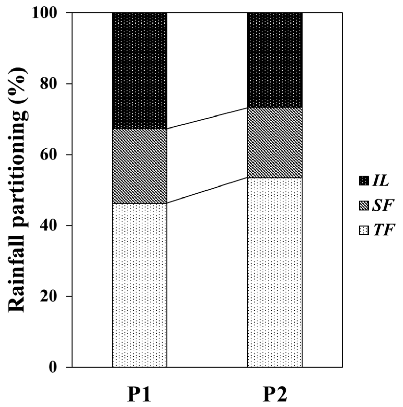
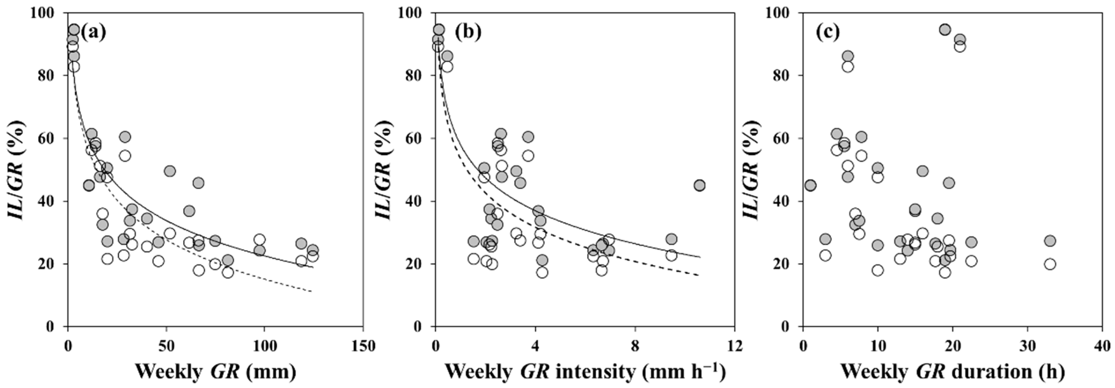
3.1. Interception Loss

During the study period (total GR: 1068.4 mm), RP of P1 and P2 differed considerably under the same SD of 2250 stems ha−1, resulting in a difference in IL/GR of 6.0% (Figure 3). For P1, TF and SF were 493.0 mm (46.1%) and 226.0 mm (21.2%), respectively, resulting in IL of 349.4 mm (32.7%). For P2, TF and SF were 570.4 mm (53.4%) and 212.5 mm (19.9%), respectively, resulting in IL of 285.5 mm (26.7%).
Weekly IL/GR of P1 ranged from 21.2% to 94.6% with a mean of 43.9% and P2 ranged from 17.2% to 94.7% with a mean of 38.9% (Figure 4). The value logarithmically decreased with the increase in weekly GR amount (mm) for P1 (R2 = 0.75) and P2 (R2 = 0.82) (Figure 4a). The value also logarithmically decreased with weekly mean GR intensity (mm h−1) for P1 (R2 = 0.63) and P2 (R2 = 0.60) (Figure 4b). However, a weak relationship was observed between weekly IL/GR and weekly GR duration (h) for P1 and P2 (R2 < 0.05) (Figure 4c). The difference in weekly IL/GR between P1 and P2 was greater with increase in weekly GR amount and weekly mean GR intensity (Figure 4a,b).

3.2. Parameters for RGAM

In the comparison of the model parameters with those of previous studies for sensitivity analysis of RGAM IL estimation [6,8], zo (stand-related parameter), pt (trunk-related parameter) and S (canopy storage-related parameter) in the present study differed from those of the previous studies, whereas the other parameters were compatible (Table 2). The value of zo was smaller because tree height was lower, pt was larger because SF/GR was larger, and S was larger because SD was larger compared with those of the previous studies.
In the comparison of the parameters between the two study plots, S and St (trunk storage-related parameter) distinctly differed, whereas the other parameters were almost identical. The parameters of P1 were larger than those of P2 (Table 2).

3.3. Performance of RGAM

The predominant component of IL estimated using the RGAM for both P1 and P2 was wet canopy evaporation after storms ceased (Id) (48.1% for P1 and 47.4% for P2), followed by wet canopy evaporation during the storms (Is) (26.2% for P1 and 32.7% for P2) (Table 3). These components accounted for 75.1% and 80.7% of the estimated IL for P1 and P2, respectively.
The RGAM underestimated cumulative IL for both P1 and P2 (Figure 5), in which the accuracy of the RGAM for P1 was lower than that for P2. For P1, the cumulative measured and estimated IL was 349.4 mm (IL/GR = 32.7%) and 278.7 mm (IL/GR = 26.1%), respectively, which resulted in a 6.6% underestimate with a cumulative IL relative error of 20.2%. For P2, the corresponding values were 285.5 mm (IL/GR = 26.7%) and 239.6 mm (IL/GR = 22.4%), respectively, which resulted in a 4.3% underestimate with a cumulative IL relative error of 16.1%. Although the estimation error of P1 was larger than that of P2, the performance of the RGAMs for P1 and P2 based on their cumulative IL relative errors were both classified as “fair” (10% < error ≤ 30%).
Lower reproducibility in P1 than P2 was observed on a weekly basis in RGAM IL estimation (Figure 6). The coefficient of determination (R2) derived from the relationship between the measured and estimated IL was 0.737 for P1 and 0.833 for P2, and the RMSE was 5.72 mm for P1 and 3.73 mm for P2.

3.4. Sensitivity Analysis

Sensitivity analysis confirmed that R ¯ (a climate parameter) showed nonlinear negative sensitivity for RGAM IL estimation, as reported previously (Table 2 [1]). In contrast, all forest structure parameters produced almost linear positive sensitivities, and the changes for both P1 and P2 were similar (Table 2 and Figure 7). Among the model parameters, zo (stand-related parameter), S (canopy storage-related parameter), and E c ¯ (evaporation-related parameter) were sensitive to RGAM IL estimation.
Among the above-mentioned three dominant parameters for IL estimation, S showed the greatest difference in sensitivity between the two study plots: when the value of S was reduced by 20%, the difference in the sensitivity of IL is 4.0% (Figure 7). In contrast, the differences in sensitivities of the parameters zo and E c ¯ were negligible between the two study plots: when the values of zo and E c ¯ were reduced by 20%, the differences in sensitivity were 1.3% and 1.3%, respectively.

4. Discussion

4.1. Applicability of RGAM IL Estimation

This study examined the applicability of the RGAM, the most commonly used IL estimation model across various forest types worldwide (as revealed in a literature review of 111 studies [13]), to unmanaged Japanese coniferous plantations with high SD laden with dead branches almost fully distributed on the stems. In the current study, “fair” performances of the RGAM were confirmed with IL relative errors of −20.2% for P1 and −16.1% for P2.
Previously, several studies applied the RGAM to Japanese coniferous plantations. Shinohara et al. [8] reported that the RGAM performed well for IL estimation in Japanese cedar plantations before thinning but may not be applicable after high-intensity selective thinning (reduction of SD by 54% and BA by 50%). However, Sun et al. [6] successfully estimated IL using the RGAM for unmanaged Japanese cypress plantations before and after high-intensity strip thinning (reduction of SD by 50% and BA by 48%) and reported “good” performances with IL relative errors of −5.7% (before thinning) and 6.8% (after thinning). Although neither the presence nor features of dead branches are described in [6], the performance could be partly underestimated by the dead branches influential on IL, which is the typical under-canopy characteristic of unmanaged Japanese cypress plantations with high SD [17,20,21].
To compare the applicability of the RGAM with the empirical model, Equation (1) was applied to P1 and P2. Komatsu et al. [11] reported that SD was the predominant parameter in IL estimation for Japanese coniferous plantations and introduced Equation (1) with a typical IL estimation error of 4.0%. Based on Equation (1), we estimated the IL/GR in P1 and P2 under the same SD of 2250 stems ha−1 in both plots to be 26.6%. The IL/GR estimate for P1 was 5.3% underestimated with a cumulative IL relative error of 18.8%, which was classified as “fair” performance. By contrast, the IL/GR estimate for P2 was only approximately 0.2% underestimated with a cumulative IL relative error of 0.6% and thus was classified as “extremely good” performance.
Although the accuracy of RGAM IL estimation in P1 and P2 was lower than that reported by Sun et al. [6], and almost the same in P2 and lower in P1 than those estimated by Equation (1), the IL estimation errors in this study could be considered acceptable because the errors lay within the “fair” performance class (10% < error ≤ 30%) [13]. The empirical model of Equation (1) showed “fair” and “extremely good” performances for IL estimation for Japanese coniferous plantations with high SD laden with dead branches, and implied high practicality with a single parameter of SD for the assessment of IL in response to forest management practices such as thinning [2,11]. This high practicality might not be surprising because of the dataset of Komatsu et al. [11]. The dataset includes several data of unmanaged Japanese cypress plantations laden with dead branches (data number 42–45 of Table 1 in [11]), which is a typical characteristic of unmanaged Japanese cypress plantations [17,20,21]. However, the relatively larger error in P1 than that in P2 using Equation (1) could occur for instances of different dead-branch structures (e.g., the number and vertical distance of dead branches [17]. The physically based RGAM showed similar accuracy as Equation (1) and could be applied for the assessment of IL in response to forest management practices affecting not only SD but also other forest stand structure parameters.
However, relatively larger errors compared with that of Sun et al. [6] were observed for RGAM IL estimation on a weekly basis in P1 and P2 where the dead branches were densely distributed (Figure 6). Measurement error can be derived from the non-above canopy meteorological data [42] and the accuracy of a relative humidity (RH) sensor [43,44]. In this study, our meteorological conditions were measured in an opening, the RH accuracy is within ±5% for RH ≥ 90%, and the wind speed was measured 7 km away from our study site. This could have partly caused our relatively larger errors. Therefore, further research is required (1) to parameterize the dead branch characteristic and (2) to measure RP on an event basis and meteorological conditions above canopies with high accurate instruments for more accurate parameters (e.g., vapor pressure deficit and aerodynamic resistance) sensitive to the Penman-Monteith equation and RGAM [45,46]. This could enable us to develop a model for a more precise estimation of IL. In this regard, we recommend TF partitioning studies (free TF, splash TF, and drip TF) measured using a disdrometer [47,48,49], and precise above-canopy measurements with calibrated instruments (e.g., rain gauges, [50]; humidity sensors, [43,44]).

4.2. Characteristics of IL Processes in the Unmanaged Plantations

The contribution of Id (IL after rainfall cessation) to the total estimated IL was predominant in both P1 and P2, accounting for approximately half of the total IL estimates (48.1% for P1 and 47.4% for P2; Table 3). This indicates that the trees store a large volume of rainwater and then evaporation of the stored rainwater is favored. This result was inconsistent with a previous study of an unmanaged Japanese cypress plantation that reported the main component of the estimated IL to be Is (Is = 62.9% [1]). Note that we assume that rainfall characteristics, such as storm size, duration, and frequency, were no different between this study and previous studies conducted in humid temperate regions.
The large S observed in the present study (Table 2) could be the reason for the predominant Id because S is the primary controller of Id in the RGAM [15,34,35]. As expected, S was the most influential sensitive parameter for IL estimation in the current study (Figure 7). Previous studies similarly reported that S is among the most sensitive parameters in the RGAM (e.g., [1,8,29,35,51]).
Compared with previous studies of Japanese coniferous plantations, the values of S observed in the present study were considerably higher (Table 2) and within the upper range of S compared with other coniferous forests (1.2–4.3 mm in Douglas fir, 0.5–1.0 mm in Pinus spp., and 1.2–2.0 mm in Picea sitchensis [37]). The substantially higher S values in the present study were possibly due to the densely distributed dead branches under canopies accounting for a considerable proportion of S [52]. The regression method used in this study has been widely used for an S estimate in diverse forest types worldwide (e.g., [8,35,38,52]). However, it might not be optimal because of the following reasons. First, it often involves a subjective selection of rain events and dry interval durations, leading to different model parameter value sets [53]. Second, the regression method does not separate S from St, resulting in higher values of S than expected if SF is not negligible [54]. Thus, further S derivation approaches for a more accurate S estimate such as automatic model parameterization procedures with optimization of S (e.g., [53]) and a new procedure to estimate S, St, and pt separately for any rain event [54] would reduce the estimated error using RGAM and improve our understanding of the impact of under-canopy structure with dead branches on S in unmanaged Japanese coniferous plantations.
Between the two study plots, IL in P1 was larger than that in P2 (Figure 3). The upper-canopy structures in P1 and P2 were statistically identical (see Section 2.1) and thus were unlikely to account for the difference in IL between the two plots. Although stand structure parameters (i.e., DBH, h, BA, and PAI) differed between the two study plots (see Section 2.1), zo (a stand-related parameter) and E c ¯ (an evaporation-related parameter), which are affected by stand structure through aerodynamic controls, did not differ between P1 and P2. Although these parameters were sensitive for RGAM IL estimation, the difference in sensitivity of these parameters between P1 and P2 was negligible. A possible reason for this result is that the difference in stand structure between P1 and P2 was insufficient for differentiation of the aerodynamic controls on IL.
The under-canopy structures of P1 and P2 were statistically different (see Section 2.1). The values of S (a canopy storage-related parameter) affected by both upper-canopy and under-canopy structures were larger in P1 than in P2 (Table 2). Although S was the dominant parameter sensitive for RGAM IL estimation together with zo and E c ¯ , S alone showed a difference in sensitivity for RGAM IL estimation between P1 and P2: when the value of S was reduced by 20%, the difference in sensitivity is 4.0% (Figure 7). The higher S in P1 than in P2 was probably due to the difference in number (56 and 47 branches per tree, respectively) and narrower vertical space (14.1 and 22.9 cm, respectively) of dead branches (Table 1 and Figure 2b). S was estimated separately from RGAM in this study. It was obtained from the measured RP data influenced by forest stand structures during rainstorms (i.e., stand structure, upper-canopy structure, and under-canopy structure with dead branches) [17,52]. Since the RGAM has no direct parameter quantifying dead branch structures, another approach such as adding new parameters of dead branch structures to the RGAM formula is needed to improve the RGAM performance for forests laden with dead branches.
Microtopography could result in differences in IL between flat areas and mountainous areas [8]. For example, Saito et al. [33] estimated IL/GR at 26% under SD of 1107 stems ha−1 in a mountainous area in a mature Japanese cedar plantation. Shinohara et al. [8] estimated IL/GR under SD of 1300 stems ha−1 in a plain area in a mature Japanese cedar plantation. The authors reported approximately half of the IL/GR of Saito et al. [33] although the two study sites were 15 km away. These results imply that IL could be different in unmanaged Japanese coniferous plantations laden with dead branches under different microtopography. Future studies examining differences in IL processes and modeling are required for evaluating the potential impacts of microtopography in unmanaged Japanese coniferous plantations laden with dead branches on forest water resources and the environment.

5. Conclusions

This study fills a knowledge gap in quantifying and estimating IL using the RGAM for Japanese coniferous plantations with high SD laden with dead branches. Although SD is a predictable parameter for IL estimation in response to forest management practices, such as thinning, for Japanese coniferous plantations, the total IL/GR between P1 and P2 differed by 6.0% (32.7% for P1 vs. 26.7% for P2) despite the same SD in the two plots. The S values in P1 and P2 were extremely high compared with those of previous studies but differed between the plots (3.94 and 3.25 mm, respectively), which were influenced by the different number of dead branches (56 and 47 branches per tree, respectively). The difference in S enables the RGAM to reflect the influence of dead branch structure on IL, leading to an acceptable RGAM performance for both P1 and P2 (“fair” IL relative errors: −20.2% vs. −16.1%) in the present study of unmanaged coniferous plantations with high SD laden with dead branches.

Author Contributions

Conceptualization, S.J., T.K., and K.O.; methodology, S.J.; formal analysis, S.J.; investigation, S.J., M.F., and K.O.; data curation, S.J.; writing—original draft preparation, S.J.; writing—review and editing, T.K., Y.S., M.F., and K.O.; supervision, K.O.; project administration, K.O.; funding acquisition, K.O. All authors have read and agreed to the published version of the manuscript.

Funding

This work is partly supported by the Japan Society for the Promotion of Science, grant numbers KAKENHI 18H04152 and KAKENHI 19H03088.

Data Availability Statement

Data sharing not applicable.

Acknowledgments

We are grateful to Kasuya Research Forest, Kyushu University, for installing a meteorological station in the study area.

Conflicts of Interest

The authors declare no conflict of interest.

References

  1. Sun, X.; Onda, Y.; Kato, H. Incident rainfall partitioning and canopy interception modeling for an abandoned Japanese cypress stand. J. For. Res. 2014, 19, 317–328. [Google Scholar] [CrossRef]
  2. Komatsu, H. Modeling evapotranspiration changes with managing Japanese cedar and cypress plantations. For. Ecol. Manag. 2020, 475, 118395. [Google Scholar] [CrossRef]
  3. Oda, T.; Egusa, T.; Ohte, N.; Hotta, N.; Tanaka, N.; Green, M.B.; Suzuki, M. Effects of changes in canopy interception on stream runoff response and recovery following clear-cutting of a Japanese coniferous forest in Fukuroyamasawa Experimental Watershed in Japan. Hydrol. Process. 2021, 35, e14177. [Google Scholar] [CrossRef]
  4. Komatsu, H.; Tanaka, N.; Kume, T. Do coniferous forests evaporate more water than broad-leaved forests in Japan? J. Hydrol. 2007, 336, 361–375. [Google Scholar] [CrossRef]
  5. Llorens, P.; Domingo, F. Rainfall partitioning by vegetation under Mediterranean conditions. A review of studies in Europe. J. Hydrol. 2007, 335, 37–54. [Google Scholar] [CrossRef]
  6. Sun, X.; Onda, Y.; Kato, H.; Gomi, K.; Komatsu, H. Effect of strip thinning on rainfall interception in a Japanese cypress plantation. J. Hydrol. 2015, 525, 607–618. [Google Scholar] [CrossRef] [Green Version]
  7. Sun, X.; Onda, Y.; Otsuki, K.; Kato, H.; Gomi, T.; Liu, X. Change in evapotranspiration partitioning after thinning in a Japanese cypress plantation. Trees 2017, 31, 1411–1421. [Google Scholar] [CrossRef]
  8. Shinohara, Y.; Levia, D.F.; Komatsu, H.; Nogata, M.; Otsuki, K. Comparative modeling of the effects of intensive thinning on canopy interception loss in a Japanese cedar (Cryptomeria japonica D. Don) forest of western Japan. Agric. For. Meteorol. 2015, 214–215, 148–156. [Google Scholar] [CrossRef]
  9. Yue, K.; De Frenne, P.; Fornara, D.A.; Van Meerbeek, K.; Li, W.; Peng, X.; Ni, X.; Peng, Y.; Wu, F.; Yang, Y.; et al. Global patterns and drivers of rainfall partitioning by trees and shrubs. Glob. Change Biol. 2021, 27, 3350–3357. [Google Scholar] [CrossRef]
  10. Teklehaimanot, Z.; Jarvis, P.G.; Ledger, D.C. Rainfall interception and boundary layer conductance in relation to tree spacing. J. Hydrol. 1991, 123, 261–278. [Google Scholar] [CrossRef]
  11. Komatsu, H.; Shinohara, Y.; Otsuki, K. Models to predict changes in annual runoff with thinning and clearcutting of Japanese cedar and cypress plantations in Japan. Hydrol. Process. 2015, 29, 5120–5134. [Google Scholar] [CrossRef] [Green Version]
  12. Crockford, R.H.; Richardson, D.P. Partitioning of rainfall into throughfall, stemflow and interception: Effect of forest type, ground cover and climate. Hydrol. Process. 2000, 14, 2903–2920. [Google Scholar] [CrossRef]
  13. Muzylo, A.; Llorens, P.; Valente, F.; Keizer, J.J.; Domingo, F.; Gash, J.H.C. A review of rainfall interception modelling. J. Hydrol. 2009, 370, 191–206. [Google Scholar] [CrossRef] [Green Version]
  14. Deguchi, A.; Hattori, S.; Park, H.T. The influence of seasonal changes in canopy structure on interception loss: Application of the revised Gash model. J. Hydrol. 2006, 318, 80–102. [Google Scholar] [CrossRef]
  15. Iida, S.; Levia, D.F.; Shimizu, A.; Shimizu, T.; Tamai, K.; Nobuhiro, T.; Kebeya, N.; Noguchi, S.; Sawano, S.; Araki, M. Intrastorm scale rainfall interception dynamics in a mature coniferous forest stand. J. Hydrol. 2017, 548, 770–783. [Google Scholar] [CrossRef]
  16. Jeong, S.; Otsuki, K.; Inoue, A.; Shinohara, Y. Marked difference of rainfall partitioning in an unmanaged coniferous plantation with high stand density. J. For. Res. 2019, 24, 107–114. [Google Scholar] [CrossRef]
  17. Jeong, S.; Otsuki, K.; Farahnak, M. Relationship between stand structures and rainfall partitioning in dense unmanaged Japanese cypress plantations. J. Agric. Meteorol. 2019, 75, 92–102. [Google Scholar] [CrossRef] [Green Version]
  18. Japan Forestry Agency. Annual Report on Trends in Forest and Forestry Fiscal Year 2017; Summary; Ministry of Agriculture, Forestry and Fisheries: Japan, Tokyo, 2018; p. 30. Available online: https://www.rinya.maff.go.jp/j/kikaku/hakusyo/29hakusyo/attach/pdf/index-1.pdf (accessed on 22 February 2022).
  19. Onda, Y.; Gomi, T.; Mizugaki, S.; Nonoda, T.; Sidle, R.C. An overview of the field and modeling studies on the effect of forest devastation on flooding and environmental issues. Hydrol. Process. 2010, 24, 527–534. [Google Scholar] [CrossRef]
  20. Fujimori, T. Dynamics of crown structure and stem growth based on knot analysis of a hinoki cypress. For. Ecol. Manag. 1993, 56, 57–68. [Google Scholar] [CrossRef]
  21. Jeong, S.; Otsuki, K. Effects of tree mortality on the estimation of stemflow yield in a self-thinning coniferous plantations. Ecohydrology 2021, 14, e2327. [Google Scholar] [CrossRef]
  22. Nanko, K.; Mizugaki, S.; Onda, Y. Estimation of soil splash detachment rates on the forest floor of an unmanaged Japanese cypress plantation based on field measurements of throughfall drop size and velocities. Catena 2008, 72, 348–361. [Google Scholar] [CrossRef] [Green Version]
  23. Shinohara, Y.; Ichinose, K.; Morimoto, M.; Kubota, T.; Nanko, K. Factors influencing the erosivity indices of raindrops in Japanese cypress plantations. Catena 2018, 171, 54–61. [Google Scholar] [CrossRef]
  24. Merriam, R. A note on the interception loss equation. J. Geophys. Res. 1960, 65, 3850–3851. [Google Scholar] [CrossRef]
  25. Zinke, P.J. Forest interception studies in the United States. In Forest Hydrology; Sopper, W.E., Lull, H.W., Eds.; Pergamon Press: Oxford, NY, USA, 1967; pp. 29–40. [Google Scholar]
  26. Rutter, A.J.; Kershaw, K.A.; Robins, P.C.; Morton, A.J. A predictive model of rainfall interception in forests, 1. Derivation of the model from observations in a plantation of Corsican pine. Agric. Meteorol. 1971, 9, 367–384. [Google Scholar] [CrossRef]
  27. Rutter, A.J.; Mortin, A.J.; Robbins, P.C. A predictive model of rainfall interception in forests. 2. Generalization of the model and comparison with observations in some coniferous and hardwood stands. J. Appl. Ecol. 1975, 12, 367–380. [Google Scholar] [CrossRef]
  28. Gash, J.H.C. An analytical model of rainfall interception in forests. Q. J. R. Meteorol. Soc. 1979, 105, 43–55. [Google Scholar] [CrossRef]
  29. Gash, J.H.C.; Lloyd, C.R.; Lachaud, G. Estimating sparse forest rainfall interception with an analytical model. J. Hydrol. 1995, 170, 79–86. [Google Scholar] [CrossRef]
  30. Calder, I.R. A stochastic model of rainfall interception. J. Hydrol. 1986, 89, 65–71. [Google Scholar] [CrossRef]
  31. Nagano, M.; Inoue, A.; Sankoda, K.; Miyazawa, Y.; Maruyama, A.; Takagi, M.; Otsuki, K. Observation of Canopy Interception Ratio in Old-aged Low-density Japanese Cypress Plantations in the Aso District, Southern Japan. J. Jpn. For. Soc. 2017, 99, 70–73. [Google Scholar] [CrossRef]
  32. Kimmins, J.P. Some statistical aspects of sampling throughfall precipitation in natural cycling studies in British Columbian coastal forests. Ecology 1973, 54, 1008–1019. [Google Scholar] [CrossRef]
  33. Saito, T.; Matsuda, H.; Komatsu, M.; Xiang, Y.; Takahashi, A.; Shinohara, Y.; Otsuki, K. Forest canopy interception loss exceeds wet canopy evaporation in Japanese cypress (Hinoki) and Japanese cedar (Sugi) plantations. J. Hydrol. 2013, 507, 287–299. [Google Scholar] [CrossRef]
  34. Pypker, T.G.; Bond, B.J.; Link, T.E.; Marks, D.; Unsworth, M.H. The importance of canopy structure in controlling the interception loss of rainfall: Examples from a young and an old-growth Douglas-fir forest. Agric. For. Meteorol. 2005, 130, 113–129. [Google Scholar] [CrossRef]
  35. Sadeghi, S.M.M.; Attarod, P.; Van Stan, J.T.; Pypker, T.G.; Dunkerley, D. Efficiency of the reformulated Gash’s interception model in semiarid afforestations. Agric. For. Meteorol. 2015, 201, 76–85. [Google Scholar] [CrossRef]
  36. Tu, L.; Xiong, W.; Wang, Y.; Yu, P.; Liu, Z.; Han, X.; Yu, Y.; Shi, Z.; Guo, H.; Li, Z.; et al. Integrated effects of rainfall regime and canopy structure on interception loss: A comparative modelling analysis for an artificial larch forest. Ecohydrology 2021, 14, e2283. [Google Scholar] [CrossRef]
  37. Link, E.T.; Unsworth, M.; Marks, D. The dynamics of rainfall interception by a seasonal temperate rainforest. Agric. For. Meteorol. 2004, 124, 171–191. [Google Scholar] [CrossRef] [Green Version]
  38. Wallace, J.; McJannet, D. On interception modelling of a lowland coastal rainforest in northern Queensland, Australia. J. Hydrol. 2006, 329, 477–488. [Google Scholar] [CrossRef]
  39. Klaassen, W.; Bosveld, F.; de Water, E. Water storage and evaporation as constituents of rainfall interception. J. Hydrol. 1998, 212–213, 36–50. [Google Scholar] [CrossRef] [Green Version]
  40. Leyton, L.; Reynolds, E.R.C.; Thompson, F.B. Rainfall interception in forests and moorland. In International Symposium on Forest Hydrology; Sooper, W.E., Lull, H.W., Eds.; Pergamon Press: Oxford, NY, USA, 1967; pp. 163–178. [Google Scholar]
  41. Nakai, T.; Sumida, A.; Daikoku, K.; Matsumoto, K.; van der Molen, M.; Kodama, Y.; Kononov, A.; Maximov, T.C.; Dolman, A.; Yabuki, H.; et al. Parameterisation of aerodynamic roughness over boreal, cool- and warm-temperate forests. Agric. For. Meteorol. 2008, 148, 1916–1925. [Google Scholar] [CrossRef] [Green Version]
  42. Pearce, A.; Gash, J.; Stewart, J. Rainfall interception in a forest stand estimated from grassland meteorological data. J. Hydrol. 1980, 46, 147–163. [Google Scholar] [CrossRef]
  43. Ingleby, B.; Moore, D.; Cloan, C.; Dunn, R. Evolution and accuracy of surface humidity reports. J. Hydrometeorol. 2013, 30, 2025–2043. [Google Scholar] [CrossRef]
  44. Murakami, S. Application of three canopy interception models to a young stand of Japanese cypress and interpretation in terms of interception mechanism. J. Hydrol. 2007, 342, 305–319. [Google Scholar] [CrossRef]
  45. Rana, G.; Katerji, N. A measurement based sensitivity analysis of the Penman-Monteith actual evapotranspiration model for crops of different height and in contrasting water satus. Theor. Appl. Climatol. 1998, 60, 141–149. [Google Scholar] [CrossRef]
  46. Pereira, F.L.; Valente, F.; David, J.S.; Jackson, N.; Minunno, F.; Gash, J.H. Rainfall interception modelling: Is the wet bulb approach adequate to estimate mean evaporation rate from wet/saturated canopies in all forest types? J. Hydrol. 2016, 534, 606–615. [Google Scholar] [CrossRef] [Green Version]
  47. Nanko, K.; Onda, Y.; Ito, A.; Moriwaki, H. Effect of canopy thickness and canopy saturation on the amount and kinetic energy of throughfall: An experimental approach. Geophys. Res. Lett 2008, 35, L05401. [Google Scholar] [CrossRef] [Green Version]
  48. Levia, D.F.; Hudson, S.A.; Llorens, P.; Nanko, K. Throughfall drop size distributions: A review and prospectus for future research. Wiley Interdiscip. Rev. Water 2017, 4, e1225. [Google Scholar] [CrossRef] [Green Version]
  49. Levia, D.F.; Nanko, K.; Amasaki, H.; Giambelluca, T.W.; Hotta, N.; Iida, S.; Mudd, R.G.; Nullet, M.A.; Sakai, N.; Shinohara, Y.; et al. Throughfall partitioning by trees. Hydrol. Process. 2019, 33, 1698–1708. [Google Scholar] [CrossRef] [Green Version]
  50. Iida, S.; Levia, D.F.; Nanko, K.; Sun, X.; Shimizu, T.; Tamaki, K.; Shinohara, Y. Correction of canopy interception loss measurements in temperate forests: A comparison of necessary adjustments among three different rain gauges based on a dynamic calibration procedure. J. Hydrometeorol. 2018, 19, 547–553. [Google Scholar] [CrossRef]
  51. Linhoss, A.C.; Siegert, C.M. A comparison of five forest interception models using global sensitivity and uncertainty analysis. J. Hydrol. 2016, 538, 109–116. [Google Scholar] [CrossRef] [Green Version]
  52. Hutchings, N.J.; Milne, R.; Crowther, J.M. Canopy storage capacity and its vertical distribution in a Sitka spruce canopy. J. Hydrol. 1988, 104, 161–171. [Google Scholar] [CrossRef]
  53. Eliades, M.; Bruggeman, A.; Djuma, H.; Christou, A.; Rovanias, K.; Lubczynski, M.W. Testing three rainfall interception models and different parameterization methods with data from an open Mediterranean pine forest. Agric. For. Meteorol. 2022, 313, 108755. [Google Scholar] [CrossRef]
  54. Valente, F.; Gash, J.H.; Nóbrega, C.; David, J.S.; Pereira, F.L. Modelling rainfall interception by an olive-grove/pasture system with a sparse tree canopy. J. Hydrol. 2019, 581, 124417. [Google Scholar] [CrossRef]
Figure 1. Photos showing general forest stand characteristics of (a) a managed Japanese cypress plantation with (1) low stand density, (2) low canopy cover, (3) rich understory vegetation, and (4) no dead branches under canopies and (b) an unmanaged Japanese cypress plantation with (1) high stand density, (2) high canopy cover, (3) sparse understory vegetation, and (4) many dead branches under canopies.
Forests 13 00657 g001
Figure 2. (a) Map showing the location of the study site in the Fukuoka prefecture, Japan, and (b-1) study plot1 and (b-2) study plot 2 in unmanaged Japanese cypress plantations with high stand density laden with dead branches under the canopy. Nlb, Ndb, and Vd denote the number of live branches, the number of dead branches, and the vertical distance of dead branches, respectively. The (b-1) and (b-2) are adapted with permission from ref. [17].
Forests 13 00657 g002
Figure 3. Rainfall partitioning into throughfall (TF), stemflow (SF), and interception loss (IL) for the study plot 1 (P1) and plot 2 (P2).
Forests 13 00657 g003
Figure 4. Relationships (a) between the ratio of interception loss (IL) to gross rainfall (GR) (IL/GR) and weekly GR, (b) between IL/GR ratio and weekly GR intensity, and (c) between IL/GR ratio and weekly GR duration obtained during the study period from April to October 2017. Grey circle and open circle denote the study plot 1 (P1) and plot 2 (P2), respectively. The solid and dash lines denote P1 and P2, respectively.
Forests 13 00657 g004
Figure 5. Cumulative total of measured and estimated interception loss (IL, mm) against cumulative gross rainfall (GR) using the reformulated Gash analytical model (RGAM). (a,b) denote the study plot1 (P1) and plot2 (P2), respectively.
Forests 13 00657 g005
Figure 6. A comparison between measured and estimated interception loss (IL) using the reformulated Gash analytical model (RGAM). (a) and (b) denote the study plot1 (P1) and plot2 (P2), respectively.
Forests 13 00657 g006
Figure 7. Sensitivity analysis of the estimated interception loss (IL) in the reformulated Gash analytical model (RGAM) in two study plots of an unmanaged Japanese cypress plantation with high stand density laden with dead branches. (a,b) denote the study plot1 (P1) and plot2 (P2), respectively. Stand-related parameter: zo, roughness length (m). Canopy-related parameters: c, canopy cover. Trunk-related parameters: pt, the proportion of rain diverted into stemflow. Canopy storage-related parameters: S, canopy storage capacity (mm). Trunk storage-related parameters: St, trunk storage capacity (mm). Evaporation-related parameter: E c ¯ , mean evaporation rate under the saturated canopy conditions per unit of canopy-covered area (mm h−1). Climate parameter: R ¯ , mean rainfall rate during the saturated canopy conditions (mm h−1).
Forests 13 00657 g007
Table 1. Forest stand structure categorized into general stand structure, stand structure, upper-canopy structure, and under-canopy structure of the unmanaged Japanese cypress plantations laden with dead branches under the same and high stand density. P1 and P2 denote each study plot. The data in this table were retrieved from [17].
Forest Stand StructureP1P2
General stand structure
a The number of trees (Ntree)50 (45 + 5)50 (45 + 5)
Tree age (years)3333
b Stand density (SD, stems ha−1)2250 (2500 − 250)2250 (2500 − 250)
Stand structure
c Diameter at breast height (DBH, cm)17.7 ± 4.120.4 ± 4.1
d Tree height (h, m)12.7 ± 2.015.4 ± 2.0
c Basal area (BA, m2 ha−1)64.985.2
e Plant area index (PAI, m2 m−2)5.6 ± 0.26.4 ± 0.2
Upper-canopy structure
f The number of live branches (Nlb)15.7 (21.8%)14.7 (23.6%)
d Canopy length (CL, m)2.8 ± 1.43.0 ± 1.1
g Canopy projection area (CPA, m2)4.8 ± 1.84.7 ± 1.9
e Canopy cover (c, %)99.3 ± 0.199.6 ± 0.1
Under-canopy structure
f The number of dead branches (Ndb)56.3 (78.2%)47.4 (76.4%)
h Vertical distance of dead branches (Vd, cm)14.1 ± 1.822.9 ± 3.8
Data are given as average ± standard deviation. a The numbers in parenthesis denote the number of standing-live trees + the number of standing-dead trees. b SD was calculated with only standing-live trees. c DBH was measured for all trees in P1 and P2 using diameter calipers; BA was calculated from the DBH. d Measured for all trees in P1 and P2 using a hypsometer (Haglȍf Vertex IV-360, Haglȍf Inc., Madison, MS, USA) by dividing the branch distribution (height of treetop, lowest live branch and lowest dead branch). e Measured at 30 points in P1 and P2, respectively, using a pair of LAI-2000 plant canopy analyzers (Li-Cor Inc., Lincoln, NE, USA). f Counted using a telescope. g Measured for all trees in P1 and P2 at the horizontal distance from the tree to the projected edge of the crown along six compass directions (N, NE, SE, S, SW, NW) using a tape measure. h calculated as 1/(the height of dead branch length (m)/Ndb) × 100. Note that PAI is measured for both leaves and branches at the same time. Accordingly, it was included in the stand structure to divide into the canopy and under-canopy structures.
Table 2. Interception parameters (forest structure parameters: stand-related, canopy-related, trunk-related, canopy storage-related, trunk storage-related, and evaporation-related parameters; and climate parameter) in the reformulated Gash analytical model (RGAM) for the present two study plots (P1 and P2), including the previous studies of Japanese coniferous plantations. SD and PAI denote stand density and plant area index, respectively.
Forest Structure ParametersClimate Parameter
StudySpeciesSDPAIStand-RelatedCanopy-RelatedTrunk-RelatedCanopy Storage-RelatedTrunk Storage-RelatedEvaporation-Related
zoacbptcSdSte E c ¯  f R ¯  g
Stems ha−1m2 m−2m mmmmmm h−1mm h−1
Present study
This study (P1)Cypress 22505.60.850.990.243.94 11.190.232.84
This study (P2)Cypress 22506.40.951.000.213.25 10.580.242.84
Previous studies
[6] *Cypress 21981.600.970.122.42 20.390.382.37
[6] **Cypress 10991.600.760.091.54 20.340.323.46
[8] *Cedar13004.84.410.980.161.34 10.610.282.75
[8] **Cedar6002.41.630.860.070.83 10.420.061.44
Asterisks * and ** denote pre-thinning and post-thinning, respectively. Forest structure parameters: a Stand-related parameter: zo, roughness length (m). b Canopy-related parameter: c, canopy cover. c Trunk-related parameter: pt, the proportion of rain diverted into stemflow. d Canopy storage-related parameter: S, canopy storage capacity (mm). e Trunk storage-related parameter: St, trunk storage capacity (mm). f Evaporation-related parameter: E c ¯ (mm h−1): mean evaporation rate during rainfall under the saturated canopy conditions per unit of canopy-covered area. Climate parameter: g  R ¯ : mean gross rainfall rate (mm h−1) during the saturated canopy conditions. Superscripts 1 and 2 denote the mean method [39] and the individual storm method [37], respectively.
Table 3. Components of estimated interception loss (IL) using the reformulated Gash analytical model (RGAM) during the growing season in the two study plots of the unmanaged Japanese cypress plantations laden with dead branches. P1 and P2 denote the study plot 1 and plot 2.
ComponentsP1P2
Modeled IL (mm)Proportion of IL (%)Estimated Error (%)Modeled IL (mm)Proportion of IL (%)Estimated Error (%)
For storms GR < GR′ (ILinsuf)
Evaporation from canopy26.29.4 22.39.3
For storms GRGR′ (ILsuf)
Wetting up the canopy (ILw)5.82.1 5.12.1
Wet canopy evaporation during the storms (ILs)73.126.2 78.332.7
Evaporation after storms ceased (ILd)134.048.1 113.647.4
Evaporation from trunks (ILt)39.714.2 20.38.5
Total estimated IL278.7100.0−20.2239.6100.0−16.1
Total measured IL349.4 285.5
Publisher’s Note: MDPI stays neutral with regard to jurisdictional claims in published maps and institutional affiliations.

