Abstract
If periodically outbreaking forest insects are a generic source of forest decline, then why do outbreaks recur more periodically than decline episodes? Do standard field survey data and proxy data systematically underestimate the complexity in herbivore population dynamics? We examine three sources of previously un-analyzed time-series data (population, defoliation, and tree-ring radial growth) for the forest tent caterpillar, Malacosoma disstria Hübner (Lepidoptera: Lasiocampidae) feeding on trembling aspen, Populus tremuloides Michx. (Salicaceae), in Minnesota, in order to answer these questions. Spatial pattern analysis of defoliation data indicated not only that outbreaks are roughly periodic, with a 10–13-y cycle, but also that important deviations from periodic led to large-scale episodes of aspen decline starting in the 1950s and 1960s, near Duluth and International Falls, respectively. By using additional data from Alberta, Canada we identify critical population and defoliation thresholds where defoliation becomes aerially detectable and impactful on tree growth. The threshold where defoliation becomes aerially detectable was found to be ~50% defoliation, corresponding to a population density of ~12 egg bands per 20 cm DBH tree (or ~20 cocoons per 3 min of collection time, or ~10 male moths per pheromone trap), and which implies a radial growth reduction on the order of 40%. We found that not all moth population peaks occur above the threshold level where defoliation is aerially detectable. Asynchronous pulses of defoliation—which are difficult to detect—produce asynchronous signatures of outbreak in tree-ring data. When these pulses occur in close conjunction with regular cycling, it can lead to outbreaks of prolonged duration that result in anomalously high tree mortality.
1. Introduction
Cyclic predator–prey populations can, in theory, be synchronized through inter-population migration [1] or spatially autocorrelated random perturbation [2]. However, there are several necessary conditions (e.g., linearity and spatial homogeneity of density-dependent recruitment; spatial homogeneity in patterns of perturbation; temporal independence among perturbations) which, unsatisfied, could lead to more complex behaviour ranging from global synchrony to regional coherence to randomness [3,4,5,6]. Thus, there are many ways in which complex patterns of nearly cyclic dynamics might arise through departures from the conditions necessary for periodic and globally synchronous “harmonic” oscillations.
The forest tent caterpillar (FTC), Malacosoma disstria Hübner (Lepidoptera: Lasiocampidae), is a periodic defoliator of broad-leaved trees throughout North America [7]. In eastern Canada, outbreaks cycle regularly with a periodicity of 9–13 years [8]. Curiously, outbreaks in the prairie provinces of western Canada have exhibited poorly synchronized, aperiodic fluctuations [9,10]. Minnesota is situated between these two regions, lying south of Manitoba and Ontario, making it an interesting place to characterize FTC dynamics.
Recurring outbreaks of FTC are thought to be the result of a deterministic host–parasitoid interaction that is subject to stochastic meteorological perturbations [11,12,13,14]; however the duration of a given outbreak cycle is determined by several factors, including climatic conditions [15] and the influence of forest landscape structure on natural enemy communities [16]. Understanding the hybrid periodic and aperiodic nature of FTC population fluctuations is important because the probability of severe forest impacts rises sharply as defoliation during long-lasting outbreaks increases from 2 to 3 or more years of heavy defoliation [17].
Trembling aspen (Populus tremuloides Michx. (Salicaceae)) is a principal host tree species consumed by FTC larvae [12], and FTC defoliation is the major factor accounting for large-scale temporal variation in aspen ring-widths, far outweighing the effects of moisture limitations [18]. Consequently, outbreaks of FTC can be roughly inferred from measurements of aspen ring-widths [19,20]. A particular concern, however, is an apparent discrepancy between the strongly decadal periodicity in defoliation data [8] versus the more complex patterns exhibited in tree-ring data [19] and in population data [14]. Although FTC defoliation appears to cycle somewhat synchronously across eastern North America, the death of host aspen trees appears to be more episodic in occurrence [17,21,22]. Resolving this discrepancy is necessary if we are to develop predictive models of insect-caused tree mortality. Do standard defoliation survey data and tree-ring proxy data under-estimate the complexity of population fluctuations surrounding major forest decline events?
There are three principal sources of time-series data used in forest insect population dynamics research—insect density data, aerial defoliation survey data, and tree-ring impact data—each of which differs in terms of the character and quality of population dynamics information they convey [23]. Population analysts prefer to study, whenever possible, population density data, because it relates most directly to the process of interest: spatial and temporal patterns and causes of change in population numbers over the course of an outbreak [3]. However, population datasets for forest insect pests are typically limited by the fact that they are (1) usually based on point-counts, in contrast to spatially extensive, spatially integrated aerial defoliation survey data, and (2) not as historically complete, temporally, as is the tree-ring record. Hence the importance of the secondary, or proxy, data types in long-term, landscape-scale pest population dynamics research [24].
In a succinct summary on the relationship between FTC population levels and observed levels of defoliation and growth impact, Hildahl & Campbell [25] stated:
The forest tent caterpillar causes injury by defoliation, but the severity of injury is determined by the number of larvae present. Low populations cause a noticeable thinning of the foliage in the upper crown. High populations strip the tree completely of foliage. Depending on the size of the tree crown, 10–20 egg bands on trembling aspen trees 12.5 cm in diameter-at-breast-height usually produce enough caterpillars to cause complete defoliation. Heavy loss of leaves for two or more years results in a general decline in the vigor of the host trees. This is accompanied by dieback of twigs and branches and a significant reduction in radial growth.[all italics yours]
The phrases we italicized highlight impact functions (e.g., “foliage thinning”, “radial growth reduction”) which are incompletely specified, from the perspective of quantitative herbivore detection. What is the precise relationship between the “number of larvae” and the “severity of injury”? How much crown foliage “thinning” (in both area and intensity) is required for detection by fixed-wing aircraft? Finally, how do either population densities or foliage thinning translate into a “significant reduction” in radial growth that may be separated reliably from other environmental signals? Computer models of herbivore impact require complete specificity in every regard.
Although one might assume that aerial defoliation survey data are more informative than are tree-ring data, the opposite could be true, depending on the parameters of the defoliation and impact detectability functions. Studying Lymantria dispar dispar on hardwoods in southern Quebec, Naidoo and Lechowicz [26] demonstrated this was the case for that system:
Our results suggest that endemic levels of gypsy moth larvae, presumably feeding at low intensities on the trees in which they were counted, can have a significant negative effect on radial growth of a preferred host. This underscores the potentially adverse consequences of gypsy moth infestations during non-outbreak years. Mason et al. [27] have reported similar reductions in growth of Douglas-fir and Grand fir due to low-intensity herbivory by Douglas-fir tussock moth and western spruce budworm.
If these defoliators—including L. dispar dispar, Douglas-fir tussock moth (Orgyia pseudotsugata (McDunnough)) and Western spruce budworm (Choristoneura occidentalis (Freeman))—are not strictly periodic in their pattern of recurrence, but are rather quasi-periodic, this could help to explain how some outbreaks might last considerably longer than others, leading to heavier insect-caused forest dieback and decline.
Minnesota and Alberta are two locations where FTC has a long history of observation, making it possible to address these questions. In this paper, we use detailed population and defoliation data from central Alberta to determine the population thresholds at which defoliation becomes “noticeable” at the ground surface and aspen radial growth reduction becomes “significant”. We then examine population detectability thresholds in both aerial defoliation survey data and tree-ring data Minnesota to address three questions. First, which method (tree-ring analysis or aerial surveys) has greater sensitivity to fluctuations in FTC populations that are critical for interpretation of spatiotemporal population dynamics? Second, are Minnesota FTC population fluctuations best characterized as simple cycles, or more complex patterns? Third, what is the relationship between patterns of defoliation impact and the occurrence of large-scale decline events? We show that two major episodes of aspen decline in Minnesota—initiated in the late 1950s and the late 1960s, near Duluth and International Falls (International Falls), respectively—are attributable to complex, quasi-periodic local outbreak behavior that is not captured in a simple, harmonic, reciprocal feedback model, and can only be discerned by careful observation and analysis.
2. Materials and Methods
Defoliation data. We examined available aerial survey data for FTC from the state of Minnesota from 1933–2011. These were subjected to a time-series analysis to estimate periodicity and evaluate autocorrelation structure, and then compared to outbreak reconstructions from a large network of tree-ring plots.
Tree-ring data. A set of seven trembling aspen tree-ring chronologies was developed over a 40,000-km2 area in the Superior National Forest (SNF) of northern Minnesota for the purpose of reconstructing historical outbreaks of FTC. These were analyzed previously by Robert et al. [20]. To this set we added two aspen tree-ring chronologies for northeastern Minnesota [28] that are key: one from the International Falls region at Kabetogama State Forest (KSF), and one from the Duluth region at Cloquet Valley State Forest (CVSF) (Figure 1). These two locations are important because the International Falls region was the site of an aspen decline episode in the 1960s–70s [29], while Duluth was at the centre of an even larger-scale aspen decline event occurring a decade earlier [17]. The full set of tree-ring data were processed in the identical manner, by using the program OUTBREAK to infer the occurrence of historical outbreaks, as described in detail in Robert et al. [20]. A split between northern (i.e., International Falls) versus northeastern (i.e., Duluth) Minnesota is relevant for a second reason, namely that the contrasting patterns in defoliation and tree-rings in the two regions could be related to previously unanalyzed population data gathered by Hodson [11], described next.
Figure 1.
Study areas in Minnesota (Hodson 1977; inset + main map) and Alberta (Roland 2005; inset only). The National Forest sample sites (dots) indicate the clustered tree-ring sample locations underpinning the seven FTC outbreak chronologies in Minnesota of Robert et al. (2020). The two State Forest sample sites (octagons) identify locations for the KSF and CVSF chronologies of Cooke et al. (2003). SNF is the Superior National Forest. KSF, CVSF, GPSF are the Kabetogama, Cloquet Valley and Grand Portage State Forests of Minnesota. “CLBGR-MHBS” for the Cooking Lake Blackfoot Grazing Reserve and Ministik Hills Bird Sanctuary of Alberta.
Population data. We examined available aerial survey data from northeastern Minnesota corresponding with moth densities estimated at 20 light-trap locations in northeastern Minnesota between 1956 and 1967 [11]. Importantly, light-trap collections include moths of both sexes. Female counts are critical to population dynamics because their densities determine egg densities and defoliation in the subsequent generation. Pheromone trap catch data of males are more common, so the unanalyzed Hodson data are exceptionally valuable.
Data analysis. The Minnesota population data, aerial defoliation records, and tree-ring data, were collated in space and time, and graphed, in order to identify thresholds at which populations become detectable and impactful on radial increment.
Alberta dataset. Accurate collation of historical data streams in time and space is critical for an accurate calibration of detection and impact thresholds. In order to supplement this exercise focused on historical data from Minnesota, we appealed to additional, modern data from the aspen parkland region of central Alberta, published in Roland [14] and Cooke [30]. These data have not been analyzed from the perspective of detectability and impact thresholds, making them an excellent fit within the broader theme of this paper.
The detailed methods of data collection are described in Cooke [30] and Roland [14]. The study area includes the Cooking Lake-Blackfoot Provincial Grazing Reserve of Alberta as the single largest lease-holder, the Ministik Hills Bird Sanctuary, and more than 100 hundred private landowners. In brief, these authors collected spatial data in 140 plots over a 400-km2 area during the FTC outbreak of 1993–95 (plus additional years varying from 1998 to 2004, while populations were endemic and rising), representing an extremely well-resolved spatial data set of: timed cocoon counts, pheromone trap catches, ground observations of defoliation, and tree-ring widths.
The relationship between ring width and defoliation levels across the Cooking Lake study grid in the year 1995 was described by linear regression. The relationship between defoliation levels and cocoon densities was described by nonlinear regression, package nlme in R. All modeling and analysis was done by using the R statistical software package, version 4.1.2 [31].
Synthesis plot. In a post-hoc synthesis of the Minnesota tree-ring data, we divided the detrended ring-width series for CVSF and KSF into outbreak versus non-outbreak intervals, and computed the inter-series covariances, sum variances, and correlations, in order to characterize and quantify the degree of pairwise synchrony in fluctuations in ring widths during each interval. These two sample plots were chosen for illustrative purposes because they are separated by a sizeable distance (120 km) and correspond with the epicenters of the aspen decline episodes reported in [17,29]. The question addressed here was whether the outbreaks that led to these decline events were synchronous or asynchronous.
3. Results
3.1. Minnesota FTC Aerial Surveys
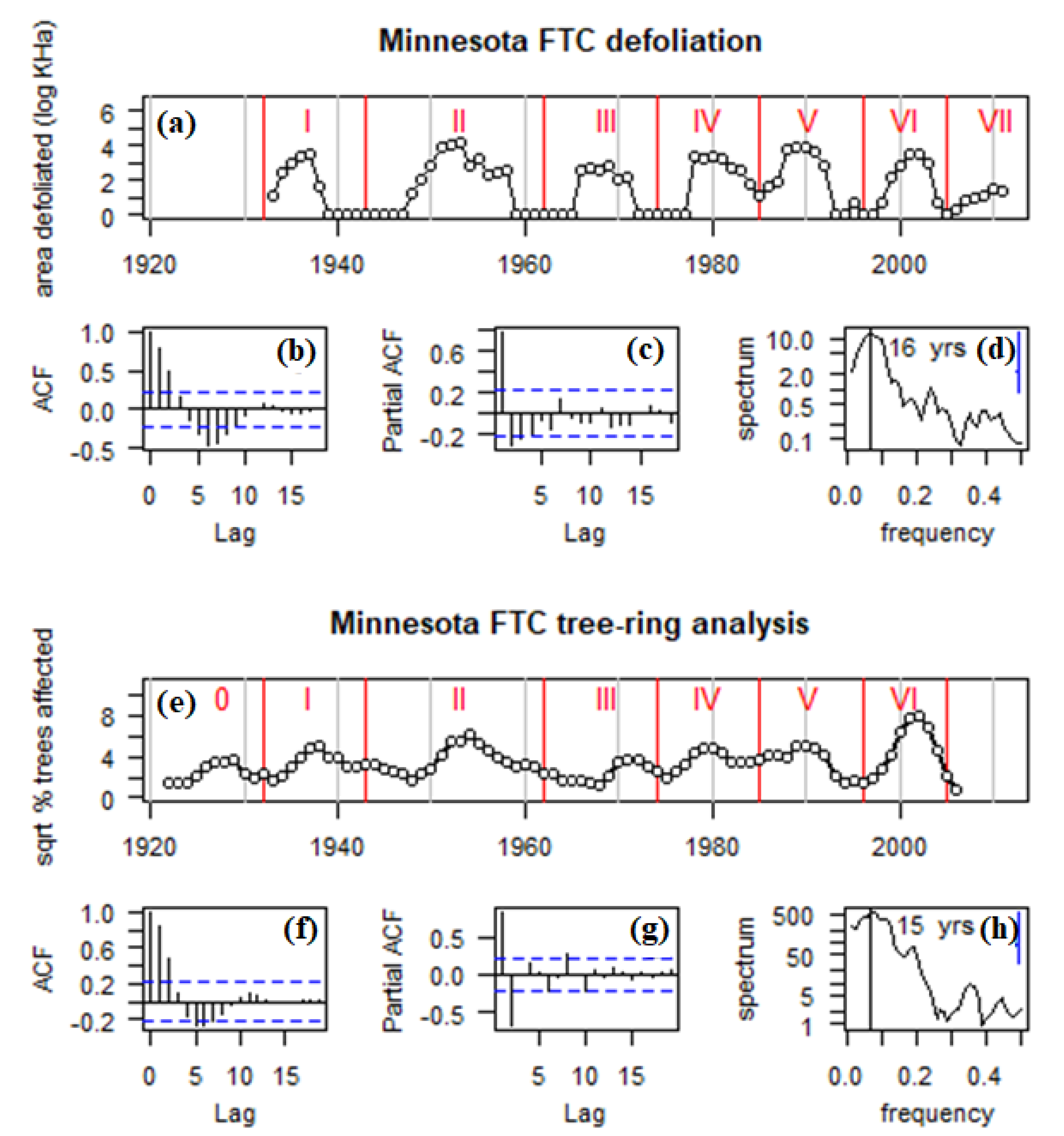
Aerial defoliation survey data from 1933–2011 indicated a highly periodic sequence of seven distinct FTC outbreaks, with a recurrence frequency of 11 years/outbreak, and numerous years between cycles where no defoliation was observed (Figure 2a). Autocorrelation analysis reflected a strongly coupled reciprocal feedback mechanism (Figure 2b,c). Spectral analysis suggested a peak periodicity of 16 years with strong variability across the 10–16-year range (Figure 2d).
Figure 2.
Time series of area impacted by FTC in Minnesota, 1922–2011. (a) Area defoliated during cycles I-VII (log10-transformed + 1). (b) Autocorrelation in area defoliated. (c) Partial autocorrelation in area defoliated. (d) Spectrum of area defoliated. (e) Square root of the % of trees affected during cycles 0-VI. (f) Autocorrelation in trees affected. (g) Partial autocorrelation in trees affected. (h) Spectrum of trees affected. Red vertical bars in (a,e) indicate cycle troughs, used as time frames in computing maps in Figure 3. The Arabic “0” is used for the first outbreak because this early outbreak is in the tree-ring record, before state-wide aerial defoliation sketch-mapping begins. Vertical lines in (d,h) indicate spectral peaks.
3.2. Growth Impact Dynamics
Trembling aspen outbreak chronologies from 1922–2006 indicated a highly periodic sequence of seven distinct FTC outbreaks, with a recurrence frequency of 12 years/outbreak, and not a single year where at least one chronology was not impacted (Figure 2e). Autocorrelation analysis reflected a strongly coupled reciprocal feedback mechanism (Figure 2f,g), with strong second order feedback, and no negative feedback appearing at the third and fourth order lags. Spectral analysis suggested a peak periodicity of 15 years with strong variability across the 8–16-year range (Figure 2h). The most intense impact cycle was VI (1996–2006), which peaked at 62% of trees affected in 2002. The least intense impact cycles were 0 (1922–32) and III (1966–71), where impact peaked at just 13% and 14% of trees affected per year. Whereas the defoliation data showed little to no sign of any sub-decadal spectral variation (Figure 2d), the tree-ring-based outbreak reconstructions indicated a minor peak of variability in the 5–6 year frequency range, which is the first harmonic of the dominant 12-y cycle (Figure 2h).
3.3. Population Detectability Thresholds
The spatial pattern of defoliation during outbreak intervals was highly aggregated during every cycle, even though the extents defoliated varied an order of magnitude between cycles, and even though the center of the area defoliated shifted around somewhat between outbreaks (Figure 3). The most extensive defoliation cycle was II (1948–58), which peaked at 14 million hectares in 1953, and was followed by the least extensive defoliation cycle, III (1966–71), which affected just 685,000 hectares in 1969, an order of magnitude difference in cycle peak extent.
Figure 3.
(a–g) Maps of cumulative area defoliated by FTC in Minnesota during each of seven outbreak cycles, I–VII, during the years 1933–2011.
Spatial patterns during these two cycles, II and III, are worth a close look for how they compare to the historical population data of Hodson [11], and the aspen decline events reported by Churchill et al. [17] and Witter et al. [29]. Annual snapshots of aerial survey data from 1948–59 (Figure 4a) indicate an FTC outbreak expanding from two epicenters—a small point of defoliation near International Falls in 1948 and a cluster of a few small pockets of defoliation in central Minnesota in 1950—to cover the entire northeastern portion of Minnesota in 1951. This was the southern extent of a more extensive outbreak occurring to the North in Ontario [8,32]. The area defoliated in 1951 declined substantially in 1952, and nearly collapsed in 1953, with the spatial pattern of spread over that time following a classic epidemiological radial spread pattern, the residual pockets of defoliation in 1953 being located in the fringe areas of west-central (e.g., Bemidji-Brainerd) and east-central (e.g., Duluth) Minnesota, around the periphery of the 1951 outbreak core. Defoliation then shifted eastward, refocusing in a couple of pockets in the Duluth area in 1954. From 1955 to 1958 defoliation lingered on within a single pocket North of Duluth, shifting a bit from year to year, and finally collapsing below the limit of detectability in 1959.
Figure 4.
Hodson’s (1977) (a) defoliation maps and (b) light-trap data for Minnesota.
In comparison, the light-trap data (Figure 4b) reveal a critical insensitivity of the aerial survey data to changes in moth density below a certain “detectability threshold”. Both the International Falls and Duluth sub-regions experienced population peaks in 1958 and 1965, the difference being that during the 1958 peak the Duluth populations were more dense than the International Falls populations, whereas in 1965 the reverse was true (Figure 4b). In other words, although populations in both sub-regions exhibited a phase-synchronized 7-year cycle, the amplitudes of the synchronized cycles were not equal in the two sub-regions. In fact, looking at the density data from traps #2 and #10—the two traps recording the greatest numbers of moths in the Duluth and International Falls sub-regions, respectively—cycle amplitude varied tremendously, with a high-amplitude cycle (peak at ~3000 moths per trap) in 1958 being followed by a low amplitude cycle (peak at ~100 moths per trap) in 1965 at trap #2, and the opposite sequence occurring in trap #10.
Comparing the population and aerial survey data during the 1958 population cycle, defoliation was observed at Duluth, but not at International Falls (Figure 4a). Yet the light-trapping data (Figure 4b) clearly indicate that there were defoliating populations reaching a peak at International Falls. Defoliation ceased being visible across both sub-regions in 1959 (Figure 4a), although population densities (again in both sub-regions) did not reach a cycle minimum until 1961 (Figure 4b).
These results show how aerial surveys are insensitive to changes in density below a certain population threshold. That detectability threshold is estimated to be between 620 adults per light trap (the lowest value observed in the last year of observed defoliation (trap #3, 1958)) and 125 adults per light trap (the highest value observed in the first year of no defoliation (trap #2, 1959)).
Based on this assumed detectability threshold, it would appear that, several years later, populations in 1965 were beginning to attain a density where defoliation should have been detectable from the air. At trap #10 (International Falls), the 620 moths-per-trap detectability threshold would almost certainly have been crossed (as early as 1964). At trap #2 (Duluth) the lower bound of the detectability threshold (125 moths per trap) would have barely been crossed. The corresponding defoliation data for 1964–67 indicate that FTC defoliation did rise to detectable levels during the 1966–71 cycle III in the International Falls region. This analysis corresponds well with Witter’s [12] remark that 1964 was the first year of visible defoliation during an outbreak cycle that eventually peaked in 1968–69.
Next, consider the corresponding tree-ring data from 1948–68 (Figure 5), in light of the foregoing analysis. There are three distinct outbreak pulses to consider (Figure 5a): the major outbreak in 1951–53 (labeled as “IIb” in Figure 5b—itself composed of the “core” outbreak pulse in 1951 and the subsequent “fringe” outbreak pulse in 1953), and the two subsequent population surges in 1958 (labeled as “IIc” in Figure 5b) and 1965 (labeled as “IIIb” in Figure 5b), neither of which resulted in state-wide defoliation, but were instead focused on Duluth and International Falls, respectively.

Figure 5.
Cooke et al.’s (2003) detrended aspen ring width data. (a) Zoom on 1948–68 time-frame. (b) Full chronologies 1926–2000, with major outbreak cycles labelled with uppercase Roman numerals as per Figure 2, and ancillary pulses labelled with lowercase Latin alphabet, a–c. (c) Spectral analysis of the two ring width chronologies. Circled values in (a) indicate the last year in which defoliation was visible and radial increment impact was “significant”: 1953 at KSF and 1959 at CVSF. Upward pointing arrows in (a) indicate major growth reductions associated with high FTC populations. Question marks in (a) indicate lesser growth reductions that were sustained but were not clearly associated with high FTC populations. Raw ring-width data in (b) are the inputs to OUTBREAK used to reconstruct outbreaks in Figure 6. Growth depression IIIb is associated with a peak in FTC moths trapped at International Falls in 1965 in Figure 4b, but does not rise to the level of a 2–5 year-long reduction in growth exceeding 1.28 (or even 0.44) standard deviations in Figure 6a, which is the standard definition of “outbreak”, and is used in Figure 2e.
As described by Cooke et al. [28], the 1951 and 1953 core and fringe pulses are clearly evident in the tree-ring width record, with the 1951 radial growth reduction at KSF/International Falls occurring 2 years before the 1953 dip at CVSF/Duluth (Figure 5a). Equally consistent with the population data: a 1958 radial growth reduction is observed at CVSF/Duluth, but not at KSF/International Falls.
Populations were starting to cross the lower limit of the defoliation detectability threshold in both sub-regions in 1963. One sees a modest radial growth reduction at Duluth in 1963, and a lesser reduction in 1963 at International Falls as well, although it is not as convincing, in part because it was preceded by even lower growth in previous years. In fact, growth at International Falls reached a local minimum two years earlier, in 1961. Similarly, instead of a 1958 minimum in growth at International Falls, the local minimum again occurred two years earlier, in 1956. These moderately sharp and sustained growth reductions, which occurred two years prior to expectation, and 4–5 years apart from one another, are indicated with question-marked arrows in Figure 5a. Until these anomalous growth reductions in 1956 and 1961 are explained, it is not clear whether populations below the low-density detectability threshold (~125 moths per trap) are capable of causing a significant growth reduction.
Nevertheless, it is worth considering the pattern of occurrence of these minor growth reductions as they relate to one another. The first feature to note is how the overall pattern of correlation in ring widths between the two series changes over time. For the 38-year period 1926–63 the correlation in detrended ring width is −0.12. For the 38-year period 1963–2000 the correlation is +0.61. The strong increase in correlation is clearly a product of the pattern of coherence in the major and minor growth reductions before and after 1963. Before 1963, there were seven growth reductions in each of the two series—yielding a periodicity of 38/7 = 5.4y; however, the minima do not coincide, and so the 5-y cycles are highly asynchronous. After 1963, the minima coincided much more closely, especially during the four major growth reductions in 1972, 1979, 1989, and 2000 (thus yielding a periodicity during that period of 38/4 = 9.5y), and so the 10-y cycles were largely synchronous.
Spectral analysis confirmed that these two dominant frequencies were the major sources of periodic variability in ring widths (Figure 5c). The decadal cycle was the major component in the KSF/International Falls series, whereas the CVSF/Duluth series exhibited a sub-decadal peak at 5y, and a decadal peak that was split between 8 y and 15 y. Thus, the two regions did not appear to be exhibiting the same growth-reduction dynamics. This is not particularly surprising given that the two regions exhibited asynchronous episodes of forest decline that were separated by 10 years ([17], v. 29).
3.4. Sensitivity in Outbreak Reconstruction
Filtering the KSF and CVSF ring-width chronologies by using the computer program OUTBREAK indicated seven major outbreak cycles over the period 1920–2000, with one outbreak cycle occurring roughly every decade (peaks numbered I-VII in Figure 6a). When the threshold was relaxed from the stringent level of −1.56 s.d., additional, inter-decadal peaks became increasingly evident. For example, the four peaks, labelled Ib, Ic, IIa, and IIc, occurring during the four periods 1937–38, 1941–42, 1947–48, and 1960–63 began to emerge as “significant” as the outbreak threshold was raised from its baseline value of −1.56 to increasingly permissive values of −1.28, −1.00, −0.72, and −0.44 respectively (Figure 6a). Although the major outbreaks occurred every decade, there were often less severe growth reductions occurring between the major decadal outbreaks. Despite their lower intensity, these reductions were nevertheless sufficient in magnitude that, depending on the threshold used to infer an outbreak, they could be interpreted as being caused by localized defoliation.

Figure 6.
Minnesota FTC outbreaks, reconstructed by filtering KSF and CVSF ring-width chronologies by using the program OUTBREAK, with the “maximum growth reduction threshold” parameter varying systematically from −1.56 to −0.44 standard deviations. (a) Percentage of chronologies exhibiting a “significant” growth reduction for a given year. Roman numerals indicate major outbreak cycles, as in Figure 2. Letter codes a-c represent more localized pulses associated with each outbreak cycle. (b) Spectra of reconstructed outbreaks in (a). Arrows indicate major (dark) and minor (light) periodic components of variability.
Spectral analysis indicated that the dominant frequency of oscillation in the reconstructed outbreak series was 9–13 years (Figure 6b, dark arrows). Sub-decadal variability in the 4–7 y range became increasingly significant as the threshold was raised from −1.56 to −0.44 (Figure 6b, light arrows). This was clearly a result of inter-decadal episodes of presumed defoliation occurring between the major decadal outbreak cycles 0 to III.
3.5. Detection and Impact Thresholds in Alberta Data
The detection and impact thresholds identified in the Minnesota data were supported and complemented by observations in Alberta (Figure 7). The Alberta analysis revealed that:
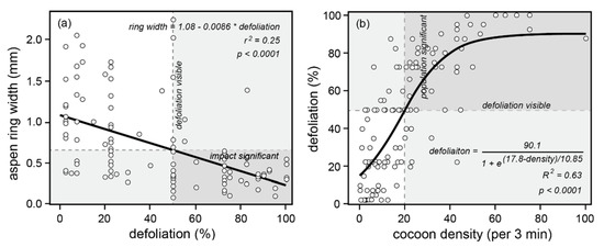
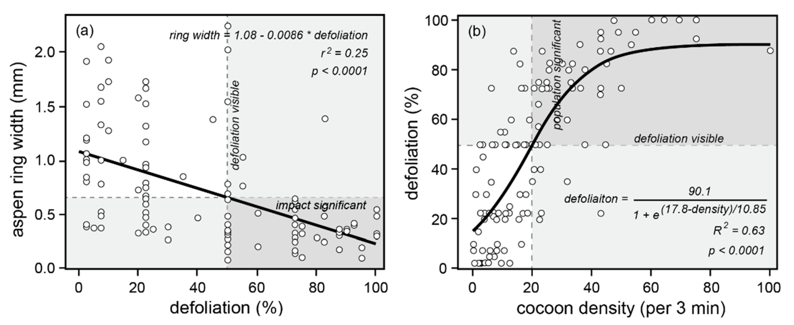
Figure 7.
Cooking Lake, Alberta population, defoliation, and impact data from 1995. The region from 50% to 100% defoliation is shaded and labelled “defoliation visible”. The upper branches of the impact curves (a,b) are also shaded, from the point at which defoliation exceeds 50%: 0.65 mm and lower in the case of (a), and 20 cocoons per 3 min and higher in (b). The dark shaded quadrants indicate the region of intersection where defoliation is visible and population impacts are “significant”. In contrast, the opposing unshaded quadrants indicate where defoliation is not visible and population impacts are not significant.
- (1)
- Approximately 50% defoliation is required to obtain a significantly reduced radial growth increment of ~0.65 mm (Figure 7a).
- (2)
- Approximately 20 cocoons (per unit area searched during a three-minute timed collection time) is required to obtain ~50% defoliation, and above 50 cocoons, the defoliation response saturates at 100% (Figure 7b).
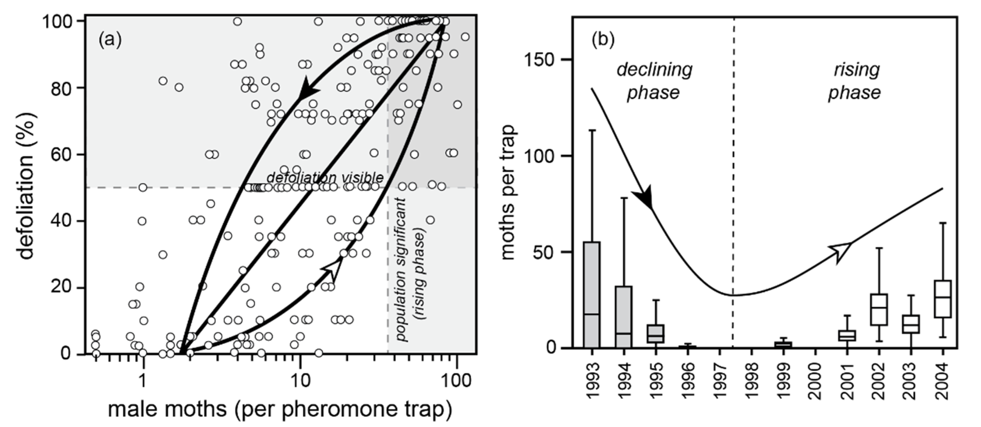
Additionally, the longer-term Alberta data reveal that:
- (3)
- The 50% defoliation threshold, in terms of adult male moth densities, varies, depending on whether the population is rising (high larval survival due to low mortality from parasitism, disease, and predation) or declining (low larval survival due to high mortality), because of the way population/outbreak cycles are driven by cyclic larval and pupal survival rates. Based on pheromone trapping of male moths, the 50% defoliation threshold is surpassed with 30+ moths per trap during the rising phase, but with fewer than 10 moths per trap during the declining phase (Figure 8a).
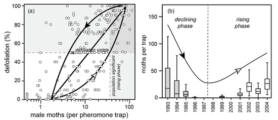 Figure 8. Cooking Lake, Alberta population and defoliation data from two partial population cycles, 1993–2004. The population phase-plane cycle in (a) represents the two curves one would expect from a rising population (white arrowhead; high late larval survival) versus a declining population (black arrowhead; low late larval survival). Given there is only one complete population cycle (among many plots) represented, this loop is a crude approximation, fitted by eye. Shading in (b) indicates years where defoliation was visible: 1993–95. Note the high spatial variation in moth densities implied in the whisker plots.
 - (4)
- The 50% defoliation threshold of detectability was exceeded from 1993–95, but still had not been exceeded during the rising phase of the next cycle, from 2002–04 (Figure 8b). This is because larval and pupal mortality is high in a collapsing cycle, requiring more larvae to produce a given number of moths, and mortality is low in the rising phase of a cycle, requiring fewer larvae to produce a given number of moths. A given number of moths therefore produces greater defoliation in the collapsing phase of the cycle than in the rising phase (as depicted in Figure 7a).
4. Discussion
4.1. Accuracy of Reconstruction
Our results show clearly that FTC in Minnesota outbreaks every 10–13 years, and during these outbreaks the extent of the areas defoliated and the intensity of defoliation is sufficient to generate significant periodic depressions in aspen radial growth measured at large scale. The level of congruent periodicity in the defoliation record and in the tree-ring record is remarkable, particularly considering that we did not attempt to “correct” aspen chronologies for the effects of precipitation on growth patterns in the traditional manner (i.e., by using a non-host chronology that supposedly captures the essence of the meteorological response signal). The reality of boreal forest insect ecology is that there are no major tree species for which there is not a significant defoliator. This result underscores the accuracy of the outbreak reconstructions analyzed by Robert et al. [20], who showed that FTC outbreaks cycle in a rather complicated matter, with significant pulses that are not synchronized with the dominant cycles.
The cycle peak intensities between the two series—defoliation and reconstructed outbreaks—correlate fairly well during cycles I–V; however this relationship starts to decay during cycle VI. Close inspection of the defoliation maps (Figure 2) reveals a rising level of fragmentation in sketch-mapped defoliation polygons during cycles VI and VII. Indeed, the ratio of the sum area of polygons and the number of polygons was large and stable through cycles I to V (Figure S1, Supplementary Materials). However, starting in 1995, the area per polygon started dropping precipitously, as mapping became less crude and more accurate because of digital recording methods and the practice of digitally excluding lakes and non-forest from sketched polygons. The resulting non-stationary estimation bias in the aerial defoliation time-series data—a bias that does not change in tree-ring data—is one reason why the tree-ring outbreak chronology indicates an intense outbreak during cycle VI, but the sketch mapping indicates an outbreak that was not as extensive as earlier outbreaks, such as during cycle II or cycle V.
4.2. Complex Cycling
The defoliation and tree-ring data streams diverge in a couple of important ways, and these deviations have practical significance, and present a number of challenges for insect disturbance ecology as practiced today. First, whereas the defoliation record reaches bottom at 0 ha in 27 of 79 years—that is 5 out of 6 inter-cycle periods—the tree-ring record indicates there is never a single year without a significant growth depression lasting 2–5 years. The minimum observed in the tree-ring record was 0.5% of samples recording an outbreak, and this was the last year of observation: 2006. Most of the other cycle minima occur at a level where 2–3% of the stems are being affected by significant growth reductions.
Second, there is a greater degree of sub-decadal periodicity in the 4–7-year frequency range in the tree-ring record, and this component becomes accentuated as the series is filtered with increasing permissiveness. This matters because the moth-trapping data in both Minnesota and Alberta indicate clearly that populations can rise to an impactful level yet still stay below the detectability of threshold of fixed-wing aerial surveyors. This result is reminiscent of observations in the L. dispar dispar system, where Naidoo & Lechowicz [26] were the first to suggest that hardwoods may be sufficiently sensitive to insect defoliation to exhibit clear impacts of endemic (i.e., sub-epidemic) population levels. Meanwhile, Johnson et al. [33] also showed that L. dispar dispar populations in some forest types in the US fluctuate at both decadal and sub-decadal periodicities. In other words, major outbreak population cycles are often followed by minor non-outbreak population cycles. This is somewhat similar to the situation described here for FTC in Minnesota, and what seems to be the case for FTC in Ontario [19] and Alberta [10]: major outbreaks are often followed and preceded by minor population cycles that, for some unknown reason, do not reach the intensity and extent of outbreak-level defoliation that is aerially detectable.
Third, the tree-ring record indicates that the annual proportion of the number of trees affected never rises higher than two-thirds. Six of the seven peaks are below 40% trees affected and the mean cycle peak intensity is just 28% trees affected. The fact that the cycle peak intensity may rise as high as 60% during cycle VI proves that this response variable is not saturating at high impact. Also worth noting is that 60% trees affected is a low number compared to spruce budworm on spruce in Quebec where 100% of trees may be affected [34]. Not only does this imply the response variable is not ever saturating, but it also means that some agent consistently prevents these cycles from become more intense and more extensive. This is true not just of the minor cycles, but even the major cycles—a result emphasized by Cooke et al. [35].
Fourth, although the regional-scale outbreak chronology (Figure 2e) is highly periodic, a close examination of individual site chronologies reveals significant departures from regular periodicity (Figure 5), and this merits deep discussion. Although the 1958 International Falls population cycle did not register in the defoliation record, there is some sign that it may have registered in the tree-ring record (Figure 5a). Although 1958 growth at KSF was not depressed, 1956 growth was. Given that the KSF tree-ring samples did not come from the exact stands sampled by Hodson’s International Falls light-traps, it seems possible that this two-year difference could be a result of local populations being out of synchrony with one another.
4.3. Defining Defoliation Detectability Thresholds
The Alberta pheromone-trap data and Minnesota light-trap data show that not all population increases necessarily lead to detectable defoliation. Forest insect populations can oscillate at levels well below the detectability threshold. This is consistent with the observation that even in core areas where FTC outbreaks are highly periodic, only half of all population cycles lead to intense and widespread defoliation [35,36].
The FTC defoliation detectability threshold is roughly 50% defoliation, which occurs at a population threshold of 20 cocoons per unit area in a three-minute timed collection. During the rising phase of the population cycle, where late larval survival is high, this corresponds to ~620 moths per light trap, or ~35 male moths per pheromone trap. With declining populations, where late larval survival is low, this corresponds to ~70 moths per light trap, or ~4 male moths per pheromone trap.
The defoliation detectability threshold is more readily defined, however, when expressed in terms of egg densities, because this eliminates the need to explicitly consider the phase of the population cycle (e.g., rising or falling, as a function of cyclic late larval and pupal mortality). Hodson [37] estimated that the 100% defoliation threshold varied with tree size, at the rate of 3 egg bands per inch of tree DBH. Half this number, or 1.5 egg bands per inch of tree DBH (11.8 egg bands per 20 cm DBH tree), should be sufficient to cause 50% defoliation. Hodson [37] estimated that egg band densities during the peak of an outbreak to range anywhere from 3.5 to 115.1 egg bands per tree (his Table 14). At the high end, assuming a fecundity of 150 larvae per egg band, this would correspond to a larval density of 1.7 × 10⁴ young larvae per tree. We did not measure egg and larval densities across the Cooking Lake grid from 1993–2004, but these numbers could be back-estimated, by fitting a life-stage survival model to the Cooking Lake data.
These population detectability threshold estimates are intended as rough approximations. Our main point in identifying these thresholds is to advance the general idea that aerial defoliation survey data from any system is likely to be inherently biased. If not, all population increases lead to defoliation that is readily detectable from the air, then defoliation records will tend to emphasize the low-frequency nature of severe outbreaks, and de-emphasize the high-frequency nature of sub-epidemic population oscillations.
4.4. Sensitivity of Aspen Ring Widths to Multifrequential Population Oscillations
We showed that when defoliation is aerially detectable (in excess of 50%), the growth reduction is likely to be significant (radial increment below 0.65 mm). However, we did not prove conclusively that significant growth reductions can occur when defoliation is not aerially detectable. There is a strong hint of such a pattern, in terms of observations at CVSF in 1965 (Figure 5a), and even more so at KSF in 1972 and 1977, when radial growth did not drop below the 0.65 mm level, yet may have been linked to moderate defoliation occurring during outbreak cycles IIIc and IV (Figure 5b). However, additional data would be required before we can conclude definitively that the tree-ring data are more sensitive to sub-epidemic population fluctuations than are aerial defoliation survey data. In particular, a more comprehensive analysis of the possible role of climatic effects is required before we can distinguish unambiguously between radial growth reductions resulting from entomological versus climatic causes. For example, the growth reduction in 1961 at KSF/International Falls (Figure 5a) is especially problematic, because FTC populations at that time were reaching their global minimum of 5.2 moths per trap. On the other hand, there were two traps, #6 and #9, where populations in 1961 attained a 1959–63 peak of 38 and 30 moths per light trap [11], his Table 3. Thus, it is not entirely clear whether the 1961 growth reduction was the result of a climatic event, such as drought, or highly localized infestations of FTC. According to Figure 5, 38 moths per light trap is below the defoliation-detectability threshold of 125 moths per trap; however it may be above the level required to cause a significant growth reduction.
The reconstructed pattern of outbreaks by using the computer program OUTBREAK confirms that the minor growth reductions in 1937–38, 1941–42, 1947–48, and 1960–63, are measurably significant. That these minor but significant growth reductions (labelled as Ib, Ic, IIa, and IIc in Figure 5 and Figure 6) occurred in between the major decadal outbreak cycles I, II, and III suggests that FTC populations in Minnesota exhibit sub-decadal and sub-epidemic population cycling. The 1960–63 growth reduction is especially noteworthy because, as just mentioned, FTC populations at that time were rising to detectable levels in some locales, such as at trap #9, where population densities reached a near-peak level of 30 moths per trap in 1961. (The primary peak of 45 moths per trap for trap #9 was reached in 1964.) Note, we are not suggesting that 30 moths per light trap is sufficient to cause a significant growth reduction; that seems unlikely. What we are suggesting is that the precise location of the light traps and the tree-ring samples may matter a great deal, such that if there is some distance between them, the comparison may not be valid. (The actual distance between Hodson’s trap #9 (near Bemidji) and our tree-ring samples from KSF (Figure 1), though large, is not really the issue. Because given the aggregative nature of FTC distributions, distances as small as tens of metres may be enough to make for an unfair comparison. Ideally, one should acquire tree ring samples from the very stands sampled by Hodson’s light-traps (Figure 4a).)
In support of this interpretation, Hodson [37] showed that the 1933–38 outbreak of FTC in Minnesota followed a similarly asynchronous pattern, with a pulse of defoliation in 1933 appearing simultaneously at Bemidji (central MN) and International Falls (north central MN), followed by a second pulse in 1938 in the extreme northeast, at Grand Portage State Forest (GPSF), near the Minnesota–Ontario border (see Figure 1 for place names). These pulses can be seen in the chain of peaks occurring during outbreak cycle I in the outbreak reconstruction (Figure 6), and a careful scan of the regional ring width chronologies (Figure 5b) reveals corresponding growth reductions occurring in the form of a prolonged reduction from 1933–37 at KSF/International Falls and a pair of brief reductions in 1934 and 1938 at CVSF/Duluth. Note the 4–5-year interval between regional-scale defoliation pulses, despite an overall, state-wide decadal outbreak cycle. These weak harmonics are not well-synchronized spatially, and tend to be more frequent when chronologies are fluctuating asynchronously (recall r = −0.12 before 1963).
The Minnesota population time-series are short; however, they are suggestive of a multifrequential oscillation, with population eruptions occurring at both decadal (9–15 y) and sub-decadal (4–7 y) time scales. Aspen ring widths and reconstructed outbreaks also appear to be multifrequential at these same time-scales. The most parsimonious interpretation of the sub-decadal 4–7 y fluctuations in aspen ring widths—which, as shown in Figure 5, are uncorrelated between regions, especially before 1963—is that they are the result of defoliation by sub-epidemic populations of a hardwood defoliator, such as the FTC. We can rule out the idea that these sub-decadal fluctuations in ring widths are a result of regional scale climatic agents, because not only are regional scale climatic perturbations more random than periodic, but they should also produce spatially correlated patterns of ring width fluctuations. The lack of regional scale coherence in ring width fluctuations precludes the action of a large-scale climatic agent (e.g., acting over 102–103 km), and instead must be a result of some local scale process (e.g., acting over 100–101 km). The one possibility that we cannot rule out is that of the endemic spatial dynamics of FTC.
4.5. Dendroecological Signatures of Outbreak
Having independent estimates of population numbers and defoliation levels, together with knowledge of defoliation detection and growth impact thresholds, allows us to take a synthetic view of the statistical properties of ring-width fluctuations during outbreak versus non-outbreak intervals. Some worthwhile patterns emerge that allow us to summarize what kinds of patterns are characteristic signatures of outbreak in spatially distributed series.
By using the International Falls/KSF and Duluth/CVSF series as an example—locations that are separated by 120 km—interval covariances and sum variances fell into six basic patterns (Figure 9). Five of these interval patterns corresponded to outbreak signals observed during cycles I, II, III, IV, and V. The sixth pattern, from 1982–86, with low variance and low covariance, was the only interval in which there was no outbreak (Figure 9e). During intervals I and II (Figure 9a,b), sum variances were high; however during I, pulses were completely out of synch, and during II, pulses at Duluth/CVSF lagged International Falls/KSF by two years. During intervals III and IV (Figure 9 f,d), sum variances were half as large (i.e., “low”); however cycle phases were in synch during III, even though amplitudes were not, yielding a high correlation, whereas in IV, the cycle at Duluth/CVSF lagged International Falls/KSF by two years (much as in II). Only interval V (Figure 9c) carried the highly correlated pattern of sustained ring-width reduction that is typically affiliated with insect outbreak. In all five cases, I-V, ring width in at least one of the two series was reduced below the 0.65 mm impact threshold identified in Figure 5 and Figure 6 as the point where aerial defoliation becomes detectable at 50%. In four of those five cases, there was significant asynchrony, with either lags of 2 years (II, IV) to 4 years (I)—yielding correlations less than zero—or amplitude mismatch (III), wherein a high positive correlation was nevertheless maintained. In all four of these cases I-IV, there was a division of patterning, where in one plot the major growth disruption was sharper, and in the other plot the growth reduction was more shallow and sustained. It is this contrast between the depth versus the breadth of spatially separated defoliation pulses that generates the asynchronous ring-width fluctuations in trembling aspen that are the defining feature of FTC outbreak. Synchronous oscillation is the exception, not the norm.
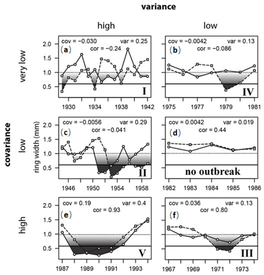
Figure 9.
Ring width patterns at KSF (solid line, circles) versus CVSF (dashed line, squares) during six different time intervals (a–f), arranged according to patterns in interval covariances and sum variances. Six signature patterns are illustrated, five of them corresponding to characteristic outbreak signals during cycles I, II, III, IV, and V. Growth reductions below the horizontal 0.65 mm impact detection threshold (~50% defoliation, Figure 7) are shaded dark grey. Lighter shading between 1.0 mm and 0.65 mm indicates the likely defoliation intensity, from undetectable (light shading) to detectable (dark shading), as suggested in Figure 5a,b and Figure 7a. The sixth pattern, from 1982–1986, with low covariance, low variance, and positive correlation, was the only interval in which there was no outbreak (no shading).
In summary, none of the patterns of growth reduction in outbreak intervals I–V is consistent with meteorological causation. The growth reductions are too large, too sustained, and very often (80% of the time) too asynchronous (either in phase or amplitude, or both). These asynchronous patterns are, instead, characteristic of insect outbreak, particularly if the herbivore’s dynamics are pulse-eruptive. The only interval where there was no outbreak was 1982–86, where ring widths never dropped below 1 mm, and yet are inter-correlated at r = 0.44 (Figure 9e). This is the standard expectation for tree-ring cross-dating. This is evidence that trembling aspen ring widths are not “complacent” in response to weather fluctuations. The lack of correlation amongst trembling aspen ring width chronologies is not a defining tree species characteristic; it is the result of an extremely dynamic herbivore having continual impact, but an impact that is often asynchronous, and not strictly periodic. This asynchronous signal of herbivory explains why the “marker years” concept applies so poorly in trembling aspen.
4.6. Relationship to Historical Forest Decline Events
If forest insect populations cycled with perfect synchrony, the duration of any given outbreak would not vary spatially. However, FTC outbreak duration does vary spatially [38], and moreover the probability of aspen forest decline is directly linked to outbreak duration, with a much larger risk of decline for outbreaks that persist as long as three years [17]. Prolonged outbreaks result in reduced transpiration rates year after year, leading to higher water table levels that contribute to the spatial pattern of accelerated stand decline [29]. Most outbreaks of FTC do not last longer than two years; however, some do, and this is particularly likely if an outbreak cycle is preceded or followed by an additional, more localized pulse of outbreak [35]. In such a case, the outbreak, locally, may endure for as many as eight years, resulting in large-scale aspen forest decline [8,21].
In fact, a close examination of two of our nine aspen tree-ring chronologies (CVSF and KSF and, located near Duluth and International Falls, respectively) indicate patterns that are episodically divergent from the regional master outbreak chronology in ways related directly to the large-scale forest decline events in Minnesota reported by Churchill et al. [17] and Witter et al. [29]. First, the CVSF series show a massive growth reduction reaching bottom in 1953, and sustained for three years, followed by a second major depression reaching bottom in 1958—both of them exceeding the defoliation detection threshold (Figure 5a)—and this coincided spatially and temporally with the decline episode studied in [17]. The earlier growth depression from 1953–55 is associated with the peaking of major cycle II, and the second is associated with the tail end of this outbreak interval (Figure 2a). Second, the KSF series show a quadruplet sequence of minor growth reductions in 1956, 1961, 1965, and 1972, the first of which falls in the cycle II interval and the last of which falls in the cycle III interval. Defoliation during cycle III was not extensive, and was in fact largely constrained the International Falls region (Figure 3)—the area reported as being in a state of decline because of a long-lasting outbreak from 1968 to 1972 [29]. The sequence of minor growth reductions is not reflected in the regional master chronology (Figure 2e), consistent with the idea that this rapid sequence of growth reductions might have been unique to the International Falls area, with two of these four pulses being too light to be detected by aerial sketch-mapping technicians, yet heavy enough to impact tree growth and long-term forest health.
These results bring into question that conventional wisdom that FTC do not kill trembling aspen trees [39]. Extensive mortality might be rare, but when major outbreak cycles are followed by a sequence of more localized population uprisings—eruptions that may not meet the intensity and extensiveness thresholds of detectability—outbreak duration will start to exceed the tree’s tolerance threshold of 2–3 years. Double-wave outbreaks may be rare; but when they do happen, their consequences for overstorey mortality and succession appear to be significant [40].
5. Conclusions
The middle of the 20th century was a golden era for forest entomology at the University of Minnesota. The detailed studies of forest tent caterpillar on aspen by Hodson, Witter, Mattson and their students and colleagues provided a wealth of information that, to this date, had not been adequately synthesized to realize its full importance. This paper was an attempt to explain the history of FTC cycling in Minnesota, but in specific relation to major decline events from the late 1950s to the early 1960s and the late 1960s to the early 1970s that, in retrospect, were decidedly non-cyclic.
If FTC populations cycle synchronously, then why is aspen forest decline not also periodic, if defoliation is a primary cause of decline? We suggest that synchronous cycling may be a useful starting paradigm for understanding the complexity in forest insect population dynamics; however we found that the actual patterns of population fluctuation are more complex than what is suggested by either the defoliation record, which is biased, or even the tree-ring record, which is subject to interpretation. Clearly, a better model is needed to account for the full range of dynamic behavior in this species. Much of population ecology research is devoted to advancing the understanding of synchronized population cycling. We suggest that it is departures from synchronous cycling that is at the heart of boreal forest decline, and so it behooves us to study departures from expectations from simple theoretical models.
Our study shows why, among the three major types of data used in insect population dynamics research—population density data, defoliation data, and tree-ring impact data—no one source should be employed to the exclusion of others. Each type of data has its advantages and disadvantages. Special attention should be paid to those rare cases such as with the FTC, where there is sufficient spatial and temporal overlap among primary and proxy data types to permit a comparative analysis. Our results suggest a need for long-term, high-resolution population studies in conjunction with high-resolution tree-ring reconstructions.
Finally, our study illustrates how it is necessary to collect accurate insect abundance data if the goal is to predict significant impacts, such as large-scale forest decline. Inaccurate data may support overly simplistic modeling paradigms, such as the theory of harmonic oscillations—which does not predict the regular occurrence of asynchronous eruptions that we observed and which were a contributing factor to large-scale forest decline events in Minnesota initiated in the 1950s and 1960s.
Supplementary Materials
The following supporting information can be downloaded at: https://www.mdpi.com/article/10.3390/f13040601/s1, Figure S1: “FTC in Minnesota”.
Author Contributions
Conceptualization, B.J.C.; methodology, B.J.C.; software, B.J.C. and L.-E.R.; formal analysis, B.J.C.; investigation, B.J.C. and L.-E.R.; writing—original draft preparation, B.J.C.; writing—review and editing, B.J.C., B.R.S. and L.-E.R. All authors have read and agreed to the published version of the manuscript.
Funding
This project was funded through a grant from the USDA Cooperative State Research, Education and Extension Service (CSREES) Managed Ecosystems program (2005-35101-16342) to Brian Sturtevant and Barry Cooke and through a grant from the US Endowment for Forest and Communities (www.usendowment.org (accessed on 11 March 2022); Project # E2014-0260) to Brian Sturtevant and Barry Cooke, both of which were used to support Louis-Etienne Robert.
Data Availability Statement
Source data for Minnesota aerial defoliation maps are available at https://www.dnr.state.mn.us/treecare/forest_health/annualreports.html (accessed on 25 May 2011). Data for Minnesota tree rings are archived at Dryad doi https://doi.org/10.5061/dryad.6wwpzgn1n (accessed on 11 April 2022). Included there are scripts for reading these data and producing Figure 2 and Figure 3. Ancillary population data in Figure 4, Figure 5, Figure 6 and Figure 7 are presented in raw form at high enough resolution to be digitized.
Acknowledgments
The authors wish to thank Francois Lorenzetti, Jeffrey Fidgen and two anonymous reviewers for manuscript review. The Figure 1 map was prepared by Jeffrey Suvada (USDA-USFS).
Conflicts of Interest
The authors declare no conflict of interest.
References
- Barbour, D.A. Synchronous Fluctuations in Spatially Separated Populations of Cyclic Forest Insects. In Population Dynamics of Forest Insects; Watt, A.D., Leather, S.R., Hunter, M.D., Kidd, N.A.C., Eds.; Intercept Limited: Andover, UK, 1990; pp. 339–346. [Google Scholar]
- Moran, P. The Statistical Analysis of the Canadian Lynx Cycle. Aust. J. Zool. 1953, 1, 291. [Google Scholar] [CrossRef]
- Royama, T. Analytical Population Dynamics; Chapman and Hall: London, UK, 1992. [Google Scholar]
- Allen, J.C.; Schaffer, W.M.; Rosko, D. Chaos Reduces Species Extinction by Amplifying Local Population Noise. Nature 1993, 364, 229–232. [Google Scholar] [CrossRef] [PubMed]
- Ranta, E.; Kaitala, V.; Lundberg, P. The Spatial Dimension in Population Fluctuations. Science 1997, 278, 1621–1623. [Google Scholar] [CrossRef] [PubMed] [Green Version]
- Blasius, B.; Huppert, A.; Stone, L. Complex Dynamics and Phase Synchronization in Spatially Extended Ecological Systems. Nature 1999, 399, 354–359. [Google Scholar] [CrossRef] [PubMed]
- Sippell, W.L. Outbreaks of the Forest Tent Caterpillar, Malacosoma disstria Hbn., a Periodic Defoliator of Broad-Leaved Trees in Ontario. Can. Entomol. 1962, 94, 408–416. [Google Scholar] [CrossRef]
- Cooke, B.J.; MacQuarrie, C.J.K.; Lorenzetti, F. The Dynamics of Forest Tent Caterpillar Outbreaks across East-Central Canada. Ecography 2012, 35, 422–435. [Google Scholar] [CrossRef]
- Hildahl, V.; Reeks, W.A. Outbreaks of the Forest Tent Caterpillar, Malacosoma disstria Hbn., and Their Effects on Stands of Trembling Aspen in Manitoba and Saskatchewan. Can. Entomol. 1960, 92, 199–209. [Google Scholar] [CrossRef]
- Cooke, B.J.; Roland, J. Early 20th Century Climate-Driven Shift in the Dynamics of Forest Tent Caterpillar Outbreaks. Am. J. Clim. Chang. 2018, 7, 253–270. [Google Scholar] [CrossRef] [Green Version]
- Hodson, A.C. Some Aspects of Forest Tent Caterpillar Population Dynamics. In Insect Ecology: Papers Presented in the A.C. Hodson Lecture Series; Kulman, H.M., Chiang, H.M., Eds.; University of Minnesota Agriculture Experiment Station, Technical Bulletin: St. Paul, MN, USA, 1977; Volume 310, pp. 5–16. [Google Scholar]
- Witter, J.A. The Forest Tent Caterpillar (Lepidoptera: Lasiocampidae) in Minnesota: A Case History Review. Great Lakes Entomol. 1979, 12, 191–197. [Google Scholar]
- Roland, J.; Mackey, B.G.; Cooke, B. Effects of Climate and Forest Structure on Duration of Forest Tent Caterpillar Outbreaks across Central Ontario, Canada. Can. Entomol. 1998, 130, 703–714. [Google Scholar] [CrossRef]
- Roland, J. Are the “Seeds” of Spatial Variation in Cyclic Dynamics Apparent in Spatially-Replicated Short Time-Series? An Example from the Forest Tent Caterpillar. Ann. Zool. Fenn. 2005, 42, 397–407. [Google Scholar]
- Daniel, C.J.; Myers, J.H. Climate and Outbreaks of the Forest Tent Caterpillar. Ecography 1995, 18, 353–362. [Google Scholar] [CrossRef]
- Roland, J.; Taylor, P.D. Insect Parasitoid Species Respond to Forest Structure at Different Spatial Scales. Nature 1997, 386, 710–713. [Google Scholar] [CrossRef]
- Churchill, G.B.; John, H.H.; Duncan, D.P.; Hodson, A.C. Long-Term Effects of Defoliation of Aspen by the Forest Tent Caterpillar. Ecology 1964, 45, 630–633. [Google Scholar] [CrossRef]
- Hogg, E. Simulation of Interannual Responses of Trembling Aspen Stands to Climatic Variation and Insect Defoliation in Western Canada. Ecol. Model. 1999, 114, 175–193. [Google Scholar] [CrossRef]
- Cooke, B.J.; Roland, J. Trembling Aspen Responses to Drought and Defoliation by Forest Tent Caterpillar and Reconstruction of Recent Outbreaks in Ontario. Can. J. For. Res. 2007, 37, 1586–1598. [Google Scholar] [CrossRef]
- Robert, L.E.; Sturtevant, B.R.; Kneeshaw, D.; James, P.M.A.; Fortin, M.J.; Wolter, P.T.; Townsend, P.A.; Cooke, B.J. Forest Landscape Structure Influences the Cyclic-eruptive Spatial Dynamics of Forest Tent Caterpillar Outbreaks. Ecosphere 2020, 11, e03096. [Google Scholar] [CrossRef]
- Candau, J.-N.; Abt, V.; Keatley, L. Bioclimatic Analysis of Declining Aspen Stands in Northeastern Ontario; Ontario Forest Research Institute, Forestry Research Report: Sault Ste-Marie, ON, Canada, 2002; Volume 154. [Google Scholar]
- Moulinier, J.; Lorenzetti, F.; Bergeron, Y. Effects of a Forest Tent Caterpillar Outbreak on the Dynamics of Mixedwood Boreal Forests of Eastern Canada. Écoscience 2013, 20, 182–193. [Google Scholar] [CrossRef]
- Régnière, J. Interpreting Historical Records. In Proceedings of the CANUSA Spruce Budworms Research Symposium, Bangor, Maine, 16–20 September 1984; Sanders, C.J., Stark, R.W., Mullins, E.J., Murphy, J., Eds.; Canadian Forest Service: Ottawa, ON, Canada, 1985; pp. 143–144. [Google Scholar]
- Swetnam, T.W.; Lynch, A.M. Multicentury, Regional-scale Patterns of Western Spruce Budworm Outbreaks. Ecol. Monogr. 1993, 63, 399–424. [Google Scholar] [CrossRef]
- Hildahl, V.; Campbell, A.E. Forest Tent Caterpillar in the Prairie Provinces; Information Report NOR-X-135; Environment Canada, Canadian Forestry Service, Northern Forest Research Centre: Edmonton, AB, Canada, 1975. [Google Scholar]
- Naidoo, R.; Lechowicz, M.J. Effects of Gypsy Moth on Radial Growth of Deciduous Trees. For. Sci. 2001, 47, 338–348. [Google Scholar]
- Mason, R.R.; Wickman, B.E.; Paul, H.G. Radial Growth Response of Douglas-Fir and Grand Fir to Larval Densities of the Douglas-Fir Tussock Moth and the Western Spruce Budworm. For. Sci. 1997, 43, 194–205. [Google Scholar] [CrossRef]
- Witter, J.A.; Mattson, W.J.; Kulman, H.M. Numerical Analysis of a Forest Tent Caterpillar (Lepidoptera: Lasiocampidae) Outbreak in Northern Minnesota. Can. Entomol. 1975, 107, 837–854. [Google Scholar] [CrossRef]
- Cooke, B.J.; Miller, W.E.; Roland, J. Survivorship Bias in Tree-Ring Reconstructions of Forest Tent Caterpillar Outbreaks Using Trembling Aspen. Tree-Ring Res. 2003, 59, 29–36. [Google Scholar]
- Cooke, B.J. Interactions between Climate, Trembling Aspen, and Outbreaks of the Forest Tent Caterpillar in Alberta. Ph.D. Dissertation, Department of Biological Sciences, University of Alberta, Edmonton, AB, Canada, 2001; 499p. [Google Scholar]
- R Core Team. R: A Language and Environment for Statistical Computing. Available online: https://cran.r-project.org/ (accessed on 11 March 2022).
- Blais, J.R.; Prentice, R.M.; Sippell, W.L.; Wallace, D.R. Effects of Weather on the Forest Tent Caterpillar Malacosoma disstria Hbn., in Central Canada in the Spring of 1953. Can. Entomol. 1955, 87, 1–8. [Google Scholar] [CrossRef]
- Johnson, D.M.; Liebhold, A.M.; Bjørnstad, O.N. Geographical Variation in the Periodicity of Gypsy Moth Outbreaks. Ecography 2006, 29, 367–374. [Google Scholar] [CrossRef]
- Boulanger, Y.; Arseneault, D.; Morin, H.; Jardon, Y.; Bertrand, P.; Dagneau, C. Dendrochronological Reconstruction of Spruce Budworm (Choristoneura fumiferana) outbreaks in southern Quebec for the last 400 years. Can. J. For. Res. 2012, 42, 1264–1276. [Google Scholar] [CrossRef]
- Cooke, B.J.; Lorenzetti, F.; Roland, J. On the Duration and Distribution of Forest Tent Caterpillar Outbreaks in East-Central Canada. J. Entomol. Soc. Ont. 2009, 140, 3–18. [Google Scholar]
- Cooke, B.J.; Lorenzetti, F. The Dynamics of Forest Tent Caterpillar Outbreaks in Québec, Canada. For. Ecol. Manag. 2006, 226, 110–121. [Google Scholar] [CrossRef]
- Hodson, A.C. An Ecological Study of the Forest Tent Caterpillar Malacosoma disstria Hbn. In Northern Minnesota; University of Minnesota Technical Bulletin: St. Paul, MN, USA, 1941; Volume 148. [Google Scholar]
- Roland, J. Large-Scale Forest Fragmentation Increases the Duration of Tent Caterpillar Outbreak. Oecologia 1993, 93, 25–30. [Google Scholar] [CrossRef]
- Schowalter, T.D. Biology and Management of the Forest Tent Caterpillar (Lepidoptera: Lasiocampidae). J. Integr. Pest Manag. 2017, 8, 24. [Google Scholar] [CrossRef] [Green Version]
- Man, R.; Rice, J.A. Response of Aspen Stands to Forest Tent Caterpillar Defoliation and Subsequent Overstory Mortality in Northeastern Ontario, Canada. For. Ecol. Manag. 2010, 260, 1853–1860. [Google Scholar] [CrossRef]


Publisher’s Note: MDPI stays neutral with regard to jurisdictional claims in published maps and institutional affiliations. |
© 2022 by the authors. Licensee MDPI, Basel, Switzerland. This article is an open access article distributed under the terms and conditions of the Creative Commons Attribution (CC BY) license (https://creativecommons.org/licenses/by/4.0/).