Strength Loss Inference Due to Decay or Cavities in Tree Trunks Using Tomographic Imaging Data Applied to Equations Proposed in the Literature

Abstract

The importance of urban forests is undeniable when considering their benefits to the environment, such as improving air quality, landscapes and breaking its monotony. However, trees are subject to failures that can cause personal and economic damage. Therefore, it is necessary to know the health conditions of the trees to define their most adequate management. Some tools are used to detect plant health conditions, such as visual analysis, tomography, and drilling resistance. In addition, some formulas based on the cavity and trunk diameter relation or the remaining trunk wall dimension are also used to infer the strength loss of a tree and its consequent risk of falling. However, these formulas have limitations, such as assuming only cavities that are always centered and not considering areas with decay. Therefore, this research evaluates whether ultrasonic tomographic imaging allows us to improve the reach of the equations proposed in the literature to infer the strength loss of trees due to the presence of cavities and decays. The results showed that ultrasonic tomographic imaging allowed the equations to be closer to real conditions of the tree trunk, such as the inclusion of wood strength reduction from decay and the displacement of internal cavities in calculating the reduction in the second moment of area.

1. Introduction

The importance of urban forests is undeniable; however, trees are subject to failure that may lead to their fall. Many targets could be hit in urban areas if they fell down, including people. Therefore, the inference of the likelihood of tree failure is very significant for the management of urban forests to define the best corrective treatment or suppression.

The falling tree risk is strongly related to their health status and the presence of inner decays, which can lead to wood strength loss and, consequently, its decline. Some methods are consolidated in the detection of the external and internal conditions of trees, such as visual analysis [1,2,3,4,5,6,7,8,9,10,11,12], the use of tomography [13,14,15,16,17], and drilling resistance [15,18,19,20,21,22,23,24].

Tree trunks are subject to efforts directly from their weight and the weight of their branches and leaves (canopy). However, the most important and significant load for the failure risk comes from the wind [25,26,27,28]. The wind load and the response of the tree to this load are dynamic in nature [29,30,31]. However, the complexity of this dynamic consideration leads many authors to propose replacing the wind action by a horizontal load applied at the center of gravity of the canopy as a simplification [28,32]. This horizontal load generates bending moments responsible for inducing stress in the tree trunk (Equation (1)). This equation allows us to verify that, concerning the same horizontal load, the trunk stress will increase if there is a reduction at the second moment of area. Likewise, Equation (1) shows that it is also possible to verify that if the wood strength decreases, the tree will be able to bear lower stress.

Σ = (M y)/I ≤ f_m

(1)

with the following definitions: σ = applied bending stress; M = bending moment; I = second moment of area; y = perpendicular distance from the fiber to the neutral axis; and f_m = bending strength of the wood.

Among the methods used to infer the falling tree risk, some equations have been proposed to quantify the strength loss using formulas [33,34,35,36]. The main limitations of these equations to estimate the reduced load-bearing capacity are assumed that the cross-section’s neutral axis corresponds to the centroid axis and only accounts for cavities and not decayed areas [37,38,39]. In this sense, Burcham et al. [38] present an interesting proposal for using ultrasonic tomography to calculate the loss of the second moment of area. This proposal considers the decay asymmetry and images produced with more grades, taking into account zones with intermediate velocity losses and not just the zones with maximum losses, usually associated with cavities.

The assessment of the stem wood strength loss is complex, so the proposed equations are based on the cavity measurement or the residual thickness of the trunk wall, which are more direct parameters. These measurements make it possible to calculate reductions at the second moment of area and infer the trunk stress increase, which the authors indirectly indicated as strength loss.

Although all equations have been developed considering important simplifications of the geometry of the trunk and cavities, Equation (2), proposed by [34], is the most conservative for indirectly inferring the strength loss (SL) from stiffness loss. This equation assumes concentric decayed and solid areas sharing the same centroid (Figure 1a) using the relation of the second moment of area of a cylinder of homogeneous and isotropic material and a hollow cylinder, both with a circular cross-section.

SL = d⁴/D⁴

(2)

with the following definitions: d = internal cavity diameter; D = trunk diameter.

Equation (3), proposed by [33], is also based on reducing the second moment of area, but the author changed the exponent (four to three). The exponent change and the choice of this specific number (3) is unclear [38].

SL = d³/D³

(3)

with the following definitions: d = internal cavity diameter; D = trunk diameter.

Equation (4), proposed by [35] and adapted from Equation (3) [33], includes the consideration of open cavities (Figure 1b). According to [39], this is very important, as these cavities remove the outer rings, which are fundamental to trunk strength.

SL = (d³ + R (D³ − d³))/D³

(4)

with the following definitions: d = internal cavity diameter; D = trunk diameter; R = ratio between the length of the cavity opening (C_c) and the trunk circumference (C).

Ref. [36] did not follow the same logic of using the reduction in the second moment of area in the inference of strength loss on the tree trunk. They used the concept of the relation between the residual wall thickness and the trunk radius (Equation (5)), also considering the trunk as a cylinder (Figure 1a).

SL = t/R_s

(5)

with the following definitions: t = residual wall thickness; R_s = trunk radius.

Thus, it is verified that all equations consider only the cavities, which effectively cause a reduction at the second moment of area, affecting the first part of Equation (1). However, trees may have deteriorated regions associated or not associated with internal cavities. Additionally, the reduction in decayed wood strength is not considered, which would affect the second part of Equation (1). The use of tomographic images is one of the ways to evaluate both cavities and deteriorated areas inside the trunk. This methodology has proven to be efficient in detecting deteriorated areas [40,41].

It should also be noted that all Equations that use reductions at the second moment of area (Equations (2)–(4)) consider that the cavity is centered. However, much higher inertia reductions occur when the cavity is eccentric, affecting the inference of the strength loss proposed by the equations.

Thus, the objective of this research was to evaluate whether the use of ultrasonic tomographic images improves the reach of the equations proposed in the literature for inferring the strength loss of trees due to the presence of cavities and decay.

2. Materials and Methods

2.1. Samples

The sample consisted of 12 cross-sections, each approximately 300 mm high, taken from the species Cenostigma pluviosum (Sibipiruna) from the campus of the Universidade de Campinas—Unicamp in the city of Campinas, São Paulo, Brazil. These cross-sections had different types and stages of decay (Figure 2).

2.2. Methodology

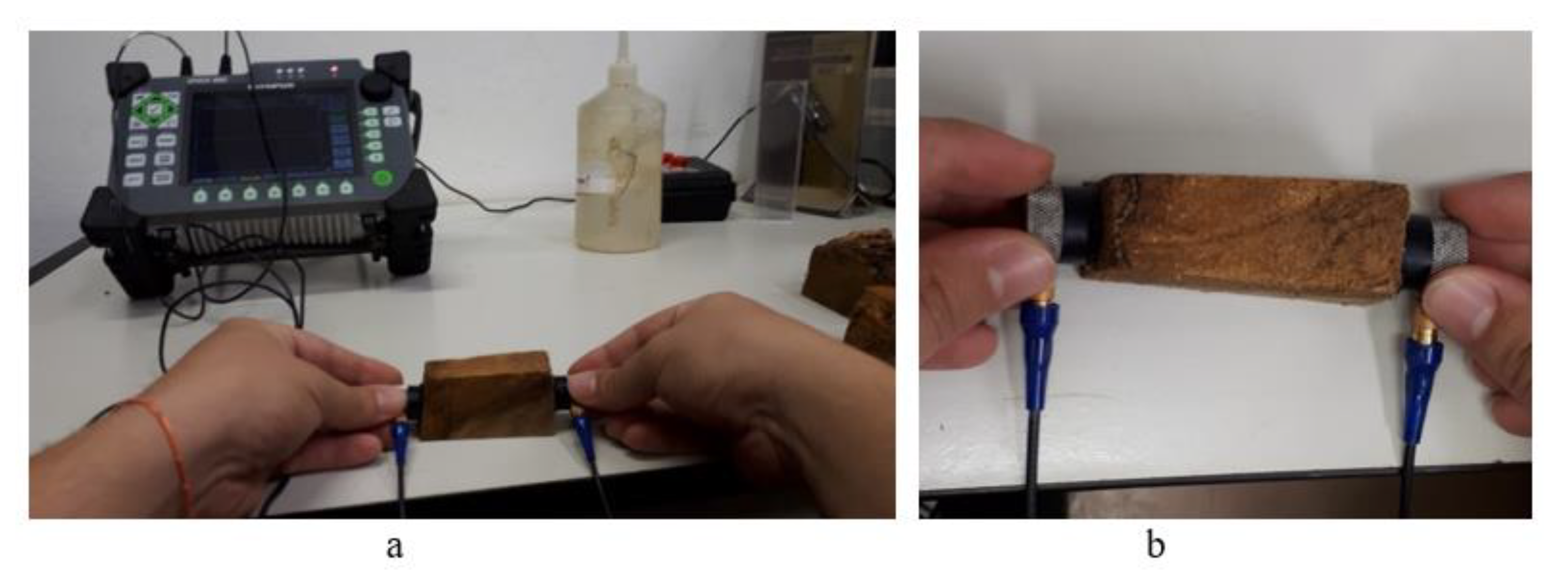
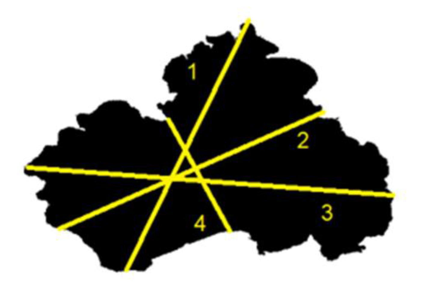
2.2.1. Ultrasound Tests on Standing Trees

The direct tests were performed at breast height (≅1.3 m from the ground) in the standing trees using ultrasound equipment (USLab, Agricef, Brazil) and 45 kHz exponential face transducers. Measurements were made using eight measuring-point diffraction mesh (Figure 3) and radial wave propagation. Holes were made in the bark at the measurement points to introduce the transducer tip ensuring its coupling to the trunk. The measurement methodology using diffraction mesh consists of positioning the emitting transducer at a measurement point and taking readings of wave propagation time while the receiving transducer sweeps all the other points. Then, the emitting transducer is positioned at the next point, repeating the procedure until it has been positioned at all diffraction mesh measurement points—this procedure generated 28 measurement routes (Figure 3).

2.2.2. Tomographic Imaging from Standing Tree Data

Regardless of the number of measurement points on the mesh, it would not be possible to have wave propagation time readings across the entire area under analysis because it is necessary to interpolate neighboring values to fill these areas and produce tomographic images. This procedure was performed using ImageWood 3.0, software developed by the LabEnd * research group (ImageWood 3.0). We adopted the interpolation system proposed by [42], with velocity compensation, which has already been used in other studies, providing good results [40,41,43,44].

To generate the tomographic image, velocity bands are associated with color bands. For homogeneous and isotropic materials, such as steel, reference velocities are generally adopted to represent the material under clear conditions. However, for wood, whose properties vary between species, within the species, and within the tree (longitudinal and radial direction), a generic reference velocity can generate great inaccuracy. Thus, the maximum velocity (Vmax) obtained in the analyzed cross-section was chosen as a reference. Based on this velocity, the ranges according to velocity variations (losses) were defined, assigning colors to elaborate the tomographic image. For the choice of velocity ranges, previous results from the literature were used [40,41,45], which was distributed into four representative velocity loss ranges: 0 to 36% of V_max to represent zones with cavities (black); 36% to 50% of V_max to represent areas with deteriorated wood (red); 50 to 80% of V_max to represent healthy areas of heartwood (brown); 80 to 100% of V_max to represent healthy areas of sapwood (yellow).

2.2.3. Preparation of Specimens

The approximately 300 mm-high cross-sections, extracted from the trees in the same position as the ultrasound measurements (Figure 3), were taken to the laboratory, where they were polished with sandpapers of different weights to highlight the areas with decays (D), healthy wood (HW) and cavities (Ca). The polished cross-sections were placed on a neutral surface to be photographed. After identifying each region, the specimens were properly removed from the cross-sections (D, HW) (Figure 4).

The specimens in the saturated condition had their volume and weight measured to calculate the apparent density in the saturated condition (ρ_sat = m_sat/V_sat). After the ultrasound tests, the specimens were kiln dried until reaching the anhydrous condition, and as soon as they did, they were weighed once again to obtain the dry mass (m_d) with which the basic density was determined (ρ_bas = m_d/V_sat).

2.2.4. Calculation of the Wood Stiffness Coefficient Taken from Different Regions of the Cross-Sections

The mechanical characterization of stiffness tests was carried out on specimens in the saturated condition to represent the tree wood more adequately. The stiffness was calculated by ultrasound, as it allows the use of small-sized test specimens (17 mm × 17 mm in cross-section and 40 mm-length in the longitudinal direction) removed from each of the regions under study. The ultrasound test, which allows the stiffness coefficient calculation, has been proposed for wood characterization, since it directly correlates with the modulus of elasticity [46,47,48] and allows testing in different dimensions of the specimen. The test was performed using ultrasound equipment (EP1000, Olympus, Tokyo, Japan) (Figure 5), due to the transducer frequency function used in the tests, which, in turn, was a function of the size of the prismatic specimen. Thus, the transducer frequency (1 MHz) was adopted to ensure that the minimum ratio between wavelength and path length was greater than three, minimizing the interferences when the wave propagation does not occur in infinite media [49]. In addition, it was ensured that the transducer diameter (13 mm) was always limited to the cross-section of the specimen, minimizing the wall effect [49].

From the ultrasound test on the specimens, the propagation time of the waves (t) was obtained, and with the path length (dimension of the specimen in the direction of the wave propagation), the propagation velocity (V) was determined. To determine the stiffness coefficient in the longitudinal direction (C_LL—Equation (6)), the basic density (ρ_bas) obtained in the specimen was used. In wood applications, the stiffness coefficient is generally calculated in the equilibrium humidity, and therefore, the apparent density in the same humidity condition is used. As the objective is the calculation of the C_LL in a saturated condition, the use of the apparent density could falsely indicate high stiffness due to the water weight and not to the effective stiffness of the material. Resulting in a contrary response to what is expected for wood [49], to which stiffness decreases as moisture increases [50].

C_LL = ρ_bas∗V²

(6)

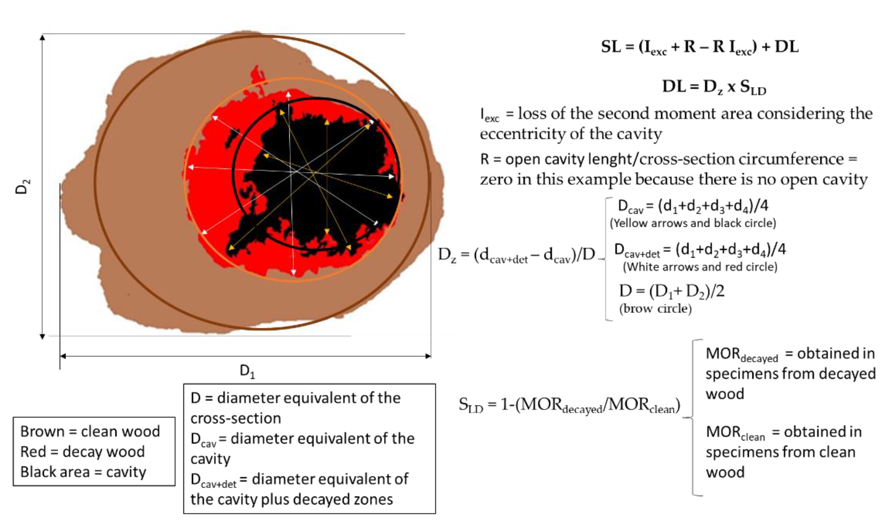
2.2.5. Determination of Data to Be Applied in Equations Proposed in the Literature

To calculate the equations proposed in the literature (Equations (2)–(5)), the necessary parameters are as follows: the deteriorated zone average diameter (d); the barkless trunk average diameter (D); the relation between the open cavity circumference and the trunk circumference (R); the thickness of the smallest wall remaining to the trunk (t); the trunk radius (R_f)—Figure 1. Thus, to obtain these parameters, the photographs of the polished cross-sections and the tomographic images were used in ImageJ software, which enabled us to measure the areas with decays and cavities and those with a smaller remaining wall thickness of the trunk when there were cross-sections with cavities.

In general, tree trunks are not regular, but as shown above, the equations proposed in the literature simplify the calculation considering a cylindrical trunk with diameter D. To consider the irregularity, the value adopted for D was the average between the largest and smallest diameters of the trunk.

For cavities, the equations also adopt a hollow cylinder. However, these cavities can be even more irregular than the trunk under real conditions, making the adoption of a cylindrical geometry imply gross errors. Thus, we sought a calculation to obtain an equivalent circular cross-section that would allow us to use the equations while minimizing errors. For this, the dimensions of decays and cavities were measured in ImageJ using the tool “Measure”, which measures the selected region using a predetermined scale, which, in the case of this research, was the dimension of the largest diameter in the real cross-section. As they are neither cylinders nor homogeneous shapes, the measurements were selected in four positions, and the average was used as an equivalent circular cross-section (Figure 6).

Two situations were considered for the calculation using Equations (2)–(5): the first using the internal cavity diameter (d) and the second using the internal cavities plus the decayed areas that surrounded the cavities (dcav + det).

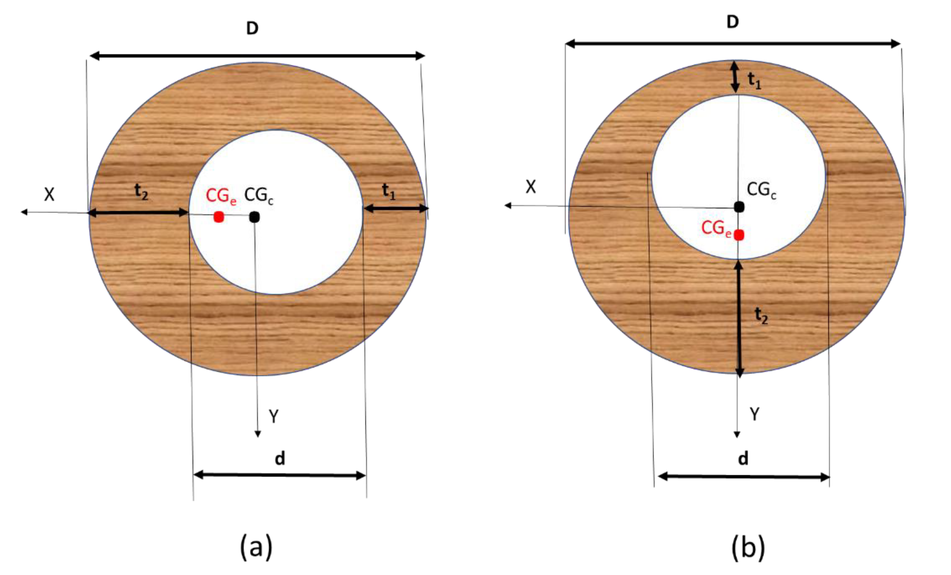
2.2.6. Calculations of Moments of Inertia Considering the Internal Cavity Centered and Noncentered on the Cross-Sections

As a simplification for the strength loss calculation, the equations proposed consider the trunk as a uniform cylinder with a central axis. When there is a cavity, they consider a hollow cylinder with a central axis (Figure 1). For this condition, the second moment of area of the solid cylinder (I_sc) with diameter D is given by Equation (7), and the second moment of area of the cross-section with hollow cylinder (I_hc) with cavity centered diameter d is given by Equation (8).

I_sc = (π D⁴)/64

(7)

I_hc = π(D⁴ − d⁴)/64

(8)

To take into account that the cavity and the cavity plus decay may not be centered, calculations were made considering the eccentricity of these regions. The eccentricity, considering in the axis X or Y, was calculated based on the thickness of the smallest wall remaining in the trunk (Figure 7). Having the eccentric position of the cavity or cavity plus the surrounding deteriorated area, we calculated the second moment of area (I) using the parallel axis theorem (I = I_c + A s²), which considers the second moment of area of that element about its own centroid (I_c), the area of the element (A) and the distance (s) from the neutral plane (x-x or y-y) to the centroid of that element.

2.2.7. Application of Data (Cross-Sections and Images) to Calculate the Stiffness Loss Considering the Centered and Noncentered Internal Cavities

For each cross-section, the data of the average diameter (D), the internal cavity (d) and the internal cavity plus the surrounding decayed (dcav + dec) were used to calculate the loss of the second moment of area considering the cavity centered or noncentered. This allows us to verify how much the consideration of the eccentricity influenced the strength loss obtained by the equations.

Equation (4) can be rewritten as:

(d³ + RD³ − Rd³)/D³ = d³/D³ + R − Rd³/D³ = (Equation (3)) + R − R ∗ (Equation (3)).

The proposed Equation (9) considers Equation (4) rewritten, but instead of the loss of the second moment of area proposed in Equation (3) (d³/D³), using concentric cavity, it proposes the calculation of the loss of the second moment area considering the eccentricity of the cavity (if there is any).

SL = I_exc + R − RI_exc

(9)

2.2.8. Proposition of an Equation including the Strength Loss of the Deteriorated Area

Equation (10) was proposed by adding to Equation (9) the loss of strength due to the deterioration (DL). The DL is obtained from Equation (14) using the decayed zone in the cross-section (D_z), Equation (11), by the average loss of strength (S_LD) obtained from results in specimens taken from clean and decayed zones (Section 2.2.4), Equation (12). As the specimens were tested by ultrasound and the results are related to stiffness (Equation (6)), the relationship between strength (MOR) and stiffness was adapted from the equation proposed by [51], to infer strength in clean and decayed wood (Equation (13)). An example of the steps used to calculate Equation (10) is shown in Figure 8.

SL = (I_exc + R − R I_exc) + DL

(10)

D_z = (d_{cav + det} − d_cav)/D

(11)

S_LD = 1 − (MOR_decayed/MOR_clean)

(12)

MOR = 22.8 + 0.0044 C_LL

(13)

DL = D_z × S_LD

(14)

3. Results

From the ultrasonic tests, the average wood stiffness (C_LL) was 12,730 MPa and 6642 MPa for the specimens taken from clear wood and decayed wood, respectively; for the same specimens, the bending strength (MOR) inferred by Equation (13) [51] was 78.8 MPa and 52.0 MPa, respectively, resulting in 34% average loss of strength (S_LD) from Equation (12).

Using the actual cross-section and the tomographic image, the parameters used in equations to calculate strength losses were obtained (

Table 1. Parameters calculated from the actual condition of the cross-sections (picture) and tomographic image.

Cross- Section	Photo	Values Referring to the Actual Condition of the Cross-Sections-Photo							Tomographic Image	Values Referring to Tomographic Images
		Cc	dcav	Dcav + Det	D	R	t	Rs		Cc	dcav	Dcav + Det	D	R	t	Rs
1		0	0	0	60.3	0	-	30.1		0	7.1	13.6	60.3	0	-	30.1
2		18.5	0	0	30.8	0.13	-	15.4		0	0	15.3	30.8	0	-	15.4
3		0	0	0	32	0	-	16		0	0	0	32	0	-	16
4		0	0	4.8	32		-	16		0	0	0	32	0	-	16
5		4.5	10.4	18.2	30.2	0.04	0	15.1		13.7	13	19.2	30.2	0.12	0	15.1
6		14.1	0	0	28.8	0.14	0	14.4		11.5	0	12.5	28.8	0.11	0	14.4
7		0	21.9	29.9	43.9	0	5.71	24.7		0	19.8	24.1	49.3	0	8.8	24.7
8		0	21.8	30.4	53	0	14.71	26.5		0	24.2	28.3	53	0	11.9	26.5
9		0	24.5	29.8	55	0	5.92	27.5		0	22.7	38.4	55	0	7.3	27.5
10		8	17.2	21.8	42.3	0.06	0	21.1		11.3	17.6	24.7	42.3	0.08	0	21.1
11		0	17.3	17.3	45.2	0	12.03	22.6		0	13.7	18.2	45.3	0	18.2	22.6
12		8.6	17.8	17.8	45.2	0.06	0	22.6		12.8	23.4	26	45.2	0.08	0	22.6

C_c = linear length of the open cavity; d_cav = equivalent cavity diameter; dcav + dec = equivalent cavity diameter + decay; D = equivalent diameter of the barkless trunk; C = trunk circumference; R = ratio between C_c and C (R = C_c/C); t = thickness of the smallest wall remaining in the cavity; R_s = trunk radius.

).

The data obtained from the 12 cross-sections fit the polynomial model presented in

Table 2. Regression models for inferring the percentage of strength loss (SL) as a function of the percentage of the trunk diameter occupied by cavity (Ca) obtained from data of the cross-sections and tomographic images applied to the equations proposed in the literature.

Regression Model	p Value	R2	Source
Data from the Cross-Sections
SL = 0.94 Ca2 − 0.49 Ca + 0.072	0.0000	0.99	[29]
SL = 1.19 Ca2 − 0.47 Ca + 0.061	0.0000	0.99	[30]
Data from the tomographic images
SL = 1.24 Ca2 − 0.50 Ca + 0.065	0.0000	0.99	[29]
SL = 1.04 Ca2 − 0.55 Ca + 0.081	0.0000	0.99	[30]

[29]: d³/D³; [30]: d⁴/D⁴.

when using Equations (2) and (3).

The values of strength loss were calculated using the data obtained from the 12 cross-sections in each of the 4 equations studied (2–5), as shown in

Table 3. Strength loss (SL in %) inferred by the equations of [34] (Equation (2)), [33] (Equation (3)); [35] (Equation (4)), and the ratio between the residual wall thickness and the trunk radius proposed by [36] (Equation (5)) using data from internal and open cavities and remaining wall thickness obtained from the cross-sections and in tomographic images.

Cross-Sections	Cross-Section Data				Tomographic Image Data
	(2)	(3)	(4)	(5)	(2)	(3)	(4)	(5)
1	0	0	0		0	0	0	-
2	0	0	13		0	0	0	-
3	0	0	0		0	0	0	-
4	0	0	0		0	0	0	-
5	1	4	8	0.00	3	8	19	0.00
6	0	0	14	0.00	0	0	11	0.00
7	4	9	9	0.23	3	6	6	0.36
8	3	7	7	0.56	4	10	10	0.45
9	4	9	9	0.22	3	7	7	0.27
10	3	7	12	0.00	3	7	15	0.00
11	2	6	6	0.53	1	3	3	0.80
12	2	6	11	0.00	7	14	21	0.00

(2): SL = d⁴/D⁴; (3): SL = d³/D³; (4): SL = (d³ + R (D³ − d³))/D³; (5): SL = t/R_s. d = equivalent cavity diameter; D = equivalent diameter of the barkless trunk; R = ratio between C_c and C (R = C_c/C), C_c = linear length of the open cavity; C = trunk circumference; t = thickness of the smallest wall remaining in the cavity; R_s = trunk radius.

.

The differences between second moments of area calculated from actual conditions (cross-sections) and tomographic images considering cavity centered and in this actual condition were calculated to be used in the equations (

Table 4. Differences (in percentage) of the second moment of area considering the cavity (if any) centered or eccentric.

	Considering Centered Cavity		Considering Actual Cavity Position
Cross-Section	Cross-Section Data	Tomographic Data	Cross-Section Data	Tomographic Data
1	0	0	0	4
2	0	0	0	0
3	0	0	0	0
4	0	0	0	0
5	1	3	24	33
6	0	0	0	0
7	4	3	14	7
8	3	4	3	5
9	4	3	15	11
10	3	3	31	32
11	2	1	3	1
12	2	7	29	41

).

The strength losses were calculated using Equations (9) and (10) proposed in this research, considering the actual position of the cavity for the calculus of the second moment of area (

Table 5. Strength loss percentage values using Equation (9) with data from actual cross-sections and tomographic images.

Cross-Section	Cross-Section Data	Tomographic Data
1	0	4
2	13	0
3	0	0
4	0	0
5	27	41
6	14	11
7	14	7
8	3	5
9	15	11
10	35	37
11	3	1
12	33	38

Equation (9): SL = I_exc + R − RI_exc; I_exc: second moment of area calculated considering eccentricity of the cavity; R = ratio between C_c and C (R = C_c/C), C_c = linear length of the open cavity; C = trunk circumference.

) and considering not only cavities but also biodeteriorations zones (

Table 6. Strength loss percentage values using Equation (10) with data from cross-sections and tomographic images.

Cross-Sections	Cross-Section Data	Tomographic Data
1	0	8
2	13	17
3	0	0
4	0	0
5	36	48
6	14	17
7	19	10
8	8	8
9	18	21
10	39	43
11	3	4
12	39	40

Equation (10): SL = (I_exc + R − R I_exc) + DL; I_exc: second moment of area calculated considering eccentricity of the cavity; R = ratio between C_c and C (R = C_c/C), C_c = linear length of the open cavity; C = trunk circumference; DL = D_z × S_LD; S_LD = 0.34; D_z = (d_{cav + det} – d_cav)/D; d_{cav + det} = equivalent diameter of the cavity + decay; d_cav = equivalent diameter of the cavity.

).

4. Discussion

Table 3 shows the strength loss calculated by using each equation studied. The data obtained from the 12 cross-sections fit a polynomial model (Table 2), as highlighted by [39], when studying Equations (2) and (3), proposed by [33,34], respectively, for the tree strength loss as a function of the internal cavity dimension. Equation (4), proposed by [35], could not be compared with the one presented by [39] because, for the actual cross-sections studied in this research, the dimension of the open cavity varied between the cross-sections. In contrast, in the graph presented by the authors, the relationship between cavity dimension and the circumference of the trunk was kept fixed at 25%.

As expected, due to the parameters involved in the equations and presented in the Introduction, the inference of strength loss is more conservative using Equation (2), followed by Equation (3) and, finally, by Equation (4)—see Table 3. Equation (5), which considers the remaining wall thickness, is the one with the greatest inferences of strength losses (Table 3).

According to [39], strength losses inferred by Equation (2) [34] from 20% to 45% indicate trees that need care, and above this value, they mean hazard trees. Strength loss predictions above 33% by Equation (3) [33] indicate hazardous trees [39]. For strength losses predicted by Equation (4) [35], values from 20% to 33% indicate a risk when the tree presents, in addition to cavities, signs of decay (cracks, trunk thickening, etc.) and above 33% if they indicate only cavities [39]. For the inference proposed by [36], Equation (5), the tree is at risk when the calculated ratio is less than 0.3 [39]. Considering these limits, none of the cross-sections analyzed in this research would be considered at risk by Equations (2)–(4) (Table 3). For Equation (5), as we always consider the smallest remaining wall thickness (t), the ratio value will already be zero whenever there is an open cavity, since t = zero. In this case, except for cross-section 7, using the tomographic data, the trees considered at risk coincided with the cross-sections (actual condition), a 92% hit (Table 3). For cross-section 7, tomography centered the cavity, causing the thickness of the remaining wall to be greater than it is. This increased the ratio value.

As expected, the loss of the second moment of area considering the centered cavity (Table 4) results in values equal to those obtained using Equation (2) (Table 3), since this equation is based only on the second moment of area variation concept. On the other hand, the loss of the second moment of area calculated with the cavity in the actual eccentric position (if this is the case of the cavity) results in higher values than those obtained with the cavity centered or with Equation (2)—see Table 4. For Equation (4), which considers the open cavity, the inferred strength losses are greater in cross-sections with these cavities (Table 3).

By replacing the portion referring to Equation (3) with the stiffness losses considering the eccentricity of the internal cavity (Equation (9)), we found that the percentage of strength loss increases (Table 5). Using the same criteria for risk consideration as in Equation (4), with a limit of 20% for trees presenting decayed areas and cavities and 33% for trees with decay, we verified that the inference of risk was coincident for the data from the tomography or actual cross-section.

Equation (10) (Table 6) shows that considering the criteria mentioned above, cross-section 9 would not be at risk (strength loss was less than 20%), according to the actual cross-section data, but would be regarding the tomographic image data. Cross-sections 5, 10 and 12 would be at risk considering data from actual cross-sections or tomography (Table 6). Cross-sections 6 and 7 would only be considered at risk using Equation (5) (Table 3). Similarly to [38], with tomography being an assistant, our results also indicate that taking into account not only cavities but also the eccentricity of the damaged part, the results of strength loss are closer to the actual condition of the trunk.

5. Conclusions

The ultrasonic tomographic images of the cross-sections improve the reach of the equations proposed in the literature for inferring the strength loss of trees due to cavities and decay.

References

1. Biondi, D.; Reissman, C.B. Evaluation of the Vigor of Urban Trees through Quantitative Parameters. Sci. Florest. 1997, 52, 17–28. [Google Scholar]
2. Gonçalves, W.; Stringheta, A.C.O.; Coelho, L.L. Analysis of urban trees for suppression purposes. Rev. Soc. Bras. Arborização Urbana 2007, 2, 1–19. [Google Scholar]
3. Matteny, H.; Clark, J. Tree risk assessment: What we know (and what we do not know). ISA 2009, 19, 28–33. [Google Scholar]
4. Schallenberger, L.S.; Araujo, A.J.; Araujo, M.N.; Deiner, L.J.; Machado, G.O. Evaluation of the condition of urban trees in the main parks and squares in the city of Irati-PR. Rev. Soc. Bras. Arborização Urbana 2010, 5, 105–123. [Google Scholar] [CrossRef]
5. Sucomine, N.M.; Sales, A. Characterization and analysis of the tree heritage of the central urban road network in the city of São Carlos-SP. Rev. Soc. Bras. Arborização Urbana 2010, 5, 128–140. [Google Scholar]
6. Smiley, E.T.; Matheny, N.; Lilly, S. Qualitative Tree Risk Assessment. Arborist News 2012, 20, 12–17. [Google Scholar]
7. Freitas, W.K.; Magalhães, L.M.S. Methods and Parameters for the Study of Vegetation with emphasis on the arboreal stratum. Floresta E Ambiente 2012, 19, 520–540. [Google Scholar] [CrossRef]
8. Teixeira, I.F.; Figueiredo, F.M.; Taborda, I.G.R.; Soares, L.M. Phytosociological analysis of Mércio Camilo square in historical center of São Gabriel, RS. Rev. Soc. Bras. Arborização Urbana 2016, 11, 1–13. [Google Scholar] [CrossRef]
9. Silva, I.R.; Oliveira, A.T.S.; Silva, L.B.O.; Baia, R.S.; Correa, T.B.C.; Martins, W.B.R. Visual diagnosis and phytosociology in the urban squares afforestation in the city of Paragominas, Pará. Rev. Soc. Bras. Arborização Urbana 2018, 13, 1–13. [Google Scholar]
10. Klein, R.W.; Koeser, A.K.; Hauer, R.J.; Hansen, G.; Escobedo, F.J. Risk Assessment and Risk Perception of Trees: A Review of Literature Relating to Arboriculture and Urban Forestry. Arboric. Urban For. 2019, 45, 23–33. [Google Scholar] [CrossRef]
11. Giacomazzi, M.; Silva, E.F.L.P.; Hardt, E. Diagnosis of urban trees on neighborhoods in the municipality of Tietê. Rev. Ra’e Ga 2020, 47, 35–48. [Google Scholar] [CrossRef]
12. Duarte, A.P.C.; Daniluk-Mosquera, G.; Gravina, V.; Vallejos-Barra, O.; Ponce-Donoso, M. Tree Risk Assessment: Component analysis of six visual methods applied in an urban park, Montevideo, Uruguay. Urban For. Urban Green. 2021, 59, 127005. [Google Scholar] [CrossRef]
13. Nicolotti, G.; Socco, L.V.; Martinis, E.; Godio, A.; Dambuelli, L. Application and comparison of three tomographic techniques for detection of decay in trees. Arboric. J. 2003, 29, 66–78. [Google Scholar] [CrossRef]
14. Gilbert, E.; Smiley, E. Picus sonic tomography for the quantification of decay in white oak (Quercus alba) and hickory (Carya spp.). J. Arboric. 2004, 30, 277–281. [Google Scholar]
15. Wang, X.; Alisson, B.R. Decay Detection in Red Oak Trees Using a Combination of Visual Inspection, Acoustic Testing, and Resistance Microdrilling. Arboric. Urban For. 2008, 34, 1–4. [Google Scholar] [CrossRef]
16. Brazee, N.; Marra, R.E.; Goecke, L.; Wassenaer, P.V. Nondestructive assessment of internal decay in three hardwood species of northeastern North America using sonic and electrical impedance tomography. Forestry 2011, 84, 33–39. [Google Scholar] [CrossRef] [Green Version]
17. Rust, S. Reproducibility of Stress Wave and Electrical Resistivity Tomography for Tree Assessment. Forests 2022, 13, 295. [Google Scholar] [CrossRef]
18. Rinn, F.; Schweingruber, F.H. Resistograph and X-ray Density Charts of Wood. Comparative Evaluation of Drill Resistance Profiles and X-ray Density Charts of Different Wood Species. Holzforschung 1996, 50, 303–311. [Google Scholar] [CrossRef]
19. Isik, F.; Li, B. Rapid assessment of wood density of live trees using the Resistograph for selection in tree improvement programs. Can. J. For. Res. 2003, 33, 2426–2435. [Google Scholar] [CrossRef]
20. Lima, J.T.; Sartório, R.C.; Trugilho, P.F.; Cruz, C.R.; Vieira, R.S. Use of the resistograph for Eucalyptus wood basic density and perforation resistance estimative. Sci. For. 2007, 75, 85–93. [Google Scholar]
21. Rinn, F. Intact-decay transitions in profiles of density-calibratable resistance drilling devices using long thin needles. Arboric. J. 2016, 38, 204–217. [Google Scholar] [CrossRef]
22. Gao, S.; Wang, X.; Wiemann, M.C.; Brashaw, B.K.; Ross, R.J.; Wang, L. A critical analysis of methods for rapid and nondestructive determination of wood density in standing trees. Ann. For. Sci. 2017, 74, 27. [Google Scholar] [CrossRef] [Green Version]
23. Vlad, R.; Zhiyanski, M.; Dinc, L.; Sidor, C.G.; Constandache, C.; Pei, G.; Ispravnic, A.; Blaga, T. Assessment of the density of wood with stem decay of Norway spruce trees using drill resistance. Comptes Rendus L’académie Bulg. Des Sci. Sci. Math. Nat. 2018, 71, 1502–1510. [Google Scholar] [CrossRef]
24. Reis, M.N.; Gonçalves, R.; Garcia, G.H.L.; Manes, L. Profiles of a Non-Calibrated Resistance Drill Compared with Deteriorated Stem Cross Sections. Arboric. Urban For. 2019, 45, 1–9. [Google Scholar] [CrossRef]
25. Gillies, J.A.; Lancaster, N.; Nickling, W.G.; Crawley, D.M. Field determination of drag forces and shear stress partitioning effects for a desert shrub (Sarcobatus vermiculatus, Greasewood). J. Geophys. Res. Atmos. 2000, 105, 24871–24880. [Google Scholar] [CrossRef]
26. Smiley, E.T.; Kane, B. The effects of pruning type on wind loading of Acer rubrum. Arboric. Urban For. 2006, 32, 33. [Google Scholar] [CrossRef]
27. Gardiner, B.; Berry, P.; Moulia, B. Wind impacts on plant growth, mechanics and damage. Plant Sci. 2016, 245, 94–118. [Google Scholar] [CrossRef] [PubMed]
28. Gonçalves, R.; Linhares, C.S.F.; Yojo, T. Drag Coefficient in Urban Trees. Trees 2020, 35, 01951. [Google Scholar] [CrossRef]
29. James, K.R.; Haritos, N.; Ades, P.K. Mechanical stability of trees under dynamic loads. Am. J. Bot. 2006, 93, 1522–1530. [Google Scholar] [CrossRef]
30. Chan, W.C.; Cui, Y.; Jadhav, S.J.; Khoo, B.C.; Lee, H.P.; Lim, C.W.C.; Gobeawan, L.; Wise, D.J.; Ge, Z.; Poh, H.J.; et al. Experimental study of wind load on tree using scaled fractal tree model. Int. J. Mod. Phys. B 2020, 34, 2040087. [Google Scholar] [CrossRef]
31. Jackson, T.D.; Sethi, S.; Dellwik, E.; Angelou, N.; Bunce, A.; Van Emmerik, T.; Duperat, M.; Ruel, J.C.; Wellpott, A.; Van Bloem, S.; et al. The motion of trees in the wind: A data synthesis. Biogeosciences 2021, 18, 4059–4072. [Google Scholar] [CrossRef]
32. Moore, J.; Maguire, D.A. Natural sway frequencies and damping ratios of trees: Concepts, review and synthesis of previous studies. Trees 2004, 18, 195–203. [Google Scholar] [CrossRef]
33. Wagener, W.W. Judging Hazard from Native Trees in California Recreational Areas: A Guide for Professional Foresters; Pacific Southwest Forest and Range Experiment Station, Forest Service, US Department of Agriculture: Berkeley, CA, USA, 1963; pp. 1–29. [Google Scholar]
34. Coder, K.D. Should you or shouldn’t you fill tree hollows? Grounds Maint. 1989, 24, 68–72. [Google Scholar]
35. Smiley, E.T.; Fraedrich, B.R. Determining strength loss from decay. Arboric. J. 1992, 18, 201–204. [Google Scholar]
36. Mattheck, C.; Kubler, H. Wood: The Internal Optimization of Trees; Springer: Berlin, Germany, 1995. [Google Scholar]
37. Ciftci, C.; Kane, B.; Brena, S.F.; Arwane, S.R. Loss in moment capacity of tree stems induced by decay. Trees 2014, 28, 517–529. [Google Scholar] [CrossRef]
38. Burcham, D.C.; Brazee, N.J.; Marra, R.E.; Kane, B. Can Sonic Tomography Predict Loss in Load-Bearing Capacity for Trees with Internal Defects? A Comparison of Sonic Tomograms with Destructive Measurements. Trees 2019, 33, 681–695. [Google Scholar] [CrossRef]
39. Kane, B.; Ryan, D.; Bloniarz, D.V. Comparing Formulas that assess strength loss due to decay in trees. J. Arboric. 2001, 27, 78–86. [Google Scholar]
40. Reis, M.N. Association of Nondestructive Methods for Tree Inspection. Master’s Thesis, University of Campinas—UNICAMP, Campinas, Brazil, 2017. [Google Scholar]
41. Palma, S.S.A. Pattern Recognition in Ultrasound Generated Images. Master’s Dissertation, University of Campinas—UNICAMP, Campinas, Brazil, 2017. [Google Scholar]
42. Du, X.; Li, S.; Li, G.; Feng, H.; Chen, S. Stress Wave Tomography of Wood Internal Defects using Ellipse-Based Spatial Interpolation and Velocity Compensation. BioResources 2015, 10, 3948–3962. [Google Scholar] [CrossRef]
43. Feng, H.; Li, G.; Fu, S.; Wang, X. Tomographic image reconstruction using an interpolation method for tree decay detection. BioResources 2014, 9, 3248–3263. [Google Scholar] [CrossRef]
44. Zeng, L.; Lin, J.; Huang, L. Interference resisting design for guided wave tomography. Smart Mater. Struct. 2013, 22, 055017. [Google Scholar] [CrossRef]
45. United States Department of Agriculture (USDA). Wood and Timber Assessment Manual, 2nd ed.; United States Department of Agriculture (USDA): Madison, WI, USA, 2014. [Google Scholar]
46. Keunecke, D.; Sonderegger, W.; Pereteanu, K.; Luthi, T.; NIiemz, P. Determination of young’s and shear moduli of common yew and Norway spruce by means of ultrasonic waves. Wood Sci. Technol. 2007, 41, 309–327. [Google Scholar] [CrossRef] [Green Version]
47. Gonçalves, R.; Trinca, A.J.; Cerri, D.G.P. Comparison of elastic constants of wood determined by ultrasonic wave propagation and static compression testing. Wood Fiber Sci. 2011, 43, 64–75. [Google Scholar]
48. Vázquez, C.; Gonçalves, R.; Bertoldo, C.; Baño, V.; Veja, A.; Crespo, J.; Guaita, M. Determination of the mechanical properties of Castanea sativa Mill. using ultrasonic wave propagation and comparison with static compression and bending methods. Wood Sci. Technol. 2015, 49, 607–622. [Google Scholar] [CrossRef]
49. Bucur, V. Acoustics of Wood, 2nd ed.; Springer: New York, NY, USA, 2006. [Google Scholar]
50. Haygreen, J.G.; Bowyer, J.L. Forest Products and Wood Science. An Introduction, 2nd ed.; Iowa State University: Ames, IA, USA, 1995. [Google Scholar]
51. Hassan, K.T.S.; Horacek, P.; Tippner, J. Evaluation of Stiffness and Strength of Scots Pine Wood Using Resonance Frequency and Ultrasonic Techniques. BioResources 2013, 8, 1634–1645. [Google Scholar] [CrossRef] [Green Version]
Figure 1. Schematic representation of a disc with a circular and concentric cavity (a) and disc with an open cavity (b). D = diameter of the disc, d = diameter of the cavity, t = residual wall thickness, Cc = circumference of the open cavity.
Forests 13 00596 g001
Figure 2. Cross-sections from the trees of Cenostigma pluviosum (Sibipiruna). d = larger diameter.
Forests 13 00596 g002
Figure 3. Scheme of the direct test with wave propagation in the radial direction (a) and 8-point diffraction mesh adopted for direct radial measurements in the trunk cross-section (b).
Forests 13 00596 g003
Figure 4. Upper image: Cross-sections after polishing showing demarcation of the healthy wood regions (HW), deteriorated wood (D) and cavity (Ca); Intermediate image: cross-section cuts in different demarcated regions; lower image: specimens taken from different demarcated regions.
Forests 13 00596 g004
Figure 5. Example of ultrasound trials performed on a prismatic specimen (a) and detailing the coupling of transducers to the specimen (b).
Forests 13 00596 g005
Figure 6. Four-position measurement scheme in areas with cavities or decay to calculate the average diameter.
Forests 13 00596 g006
Figure 7. Schematic representation of a disc with a circular cavity with eccentricity in axe X (a) and with eccentricity in axe Y (b). t1 and t2 = thickness of the wall remaining; CGc = center of gravity considering cavity centered (in black); CGe = center of gravity considering cavity with eccentricity (in red).
Forests 13 00596 g007
Figure 8. Example of the steps used to calculate Equation (10).
Forests 13 00596 g008