Abstract
Urban areas are experiencing major changes and facing significant sustainability challenges. Many cities are undergoing a transition towards a post-industrial phase and need to consider the regeneration of brownfield sites. Nature-Based Solutions (NBSs) are increasingly considered as tools for supporting this transition and promoting sustainable development by delivering multiple ecosystem services (ESs). Although the potential of NBSs as a cost-effective enabler of urban sustainability has been recognized, their implementation faces numerous barriers. The effective assessment of benefits delivered by urban NBSs is considered by existing literature as one of them. In order to contribute to filling this knowledge gap, we analyzed two alternative NBS-based intervention scenarios—i.e., (1) an urban forest and (2) meadows with sparse trees—for the redevelopment of an urban brownfield area within the municipality of Brescia (Northern Italy). Nine ESs were assessed both in biophysical and economic terms via a combination of modeling (InVEST, i-Tree and ESTIMAP) and traditional estimation methods. The results show that both scenarios improve ES stock and flow compared to the baseline, ensuring annual flows ranging between 140,000 and 360,000 EUR/year. Scenario 1 shows higher values when single ESs are considered, while scenario 2 shows higher total values, as it also accounts for the phytoremediation capacity that is not considered under the first scenario. All in all, regulating ESs represent the bulk of estimated ESs, thus highlighting the potential of proposed NBSs for improving urban resilience. The ES assessment and valuation exercise presented within this paper is an example of how research and practice can be integrated to inform urban management activities, and provide inputs for future decision making and planning regarding urban developments.
1. Introduction
Urban areas are experiencing major changes and facing significant environmental, social and economic sustainability challenges. On the one hand, the world is undergoing the largest wave of urban growth in history [1]. Urban areas have expanded in recent decades and so has the number of people living within them: more than half of the world’s population now lives in towns and cities, and that proportion will continue to grow in coming decades [2]. At the same time, shrinking cities—i.e., densely populated urban areas that faced a population loss and are undergoing economic transformation (e.g., de-industrialization, internal migration), with some symptoms of a structural crisis—are becoming a common phenomenon in many regions, particularly in Europe, North America and Japan [3]. Concerns about the sustainability of cities and urban areas have emerged accordingly [4,5], as witnessed by, among others, the 2030 Agenda for Sustainable Development; the latter includes Sustainable Development Goal 11, which aims to “Make cities and human settlements inclusive, safe, resilient and sustainable” [6]; the world Forum on Urban Forests [7]; and the UN New Urban Agenda [8]. Nature-Based Solutions (NBSs)—an emerging umbrella concept that incorporates different forms of nature-based (i.e., green) interventions [9]—can contribute to addressing ecological, social and economic sustainability challenges in urban areas [4,10,11]. Although there is not a univocal definition for NBSs and diverse perspectives on this concept have emerged [12,13], the term is increasingly integrated within policies and research activities, with a potential opening for transformational pathways towards sustainable societal development [14]. By supporting ecosystem processes and structures, such as the presence and features of a certain habitat (e.g., a forest, its species composition, and canopy characteristics), NBSs can deliver a broad range of ecosystem services (ES); these are ecosystem outputs in terms of material (e.g., wood for energy) and immaterial products and services (e.g., aesthetic view), targeting and benefiting various social groups and, ultimately, contributing to quality of life and people’s wellbeing [15,16,17]. The benefits of ESs can be understood as something that changes people’s wellbeing in terms of, for instance, health, security, or social relations [17]. These changes can be perceived as important by ES beneficiaries who, therefore, assign a value to them—in monetary and non-monetary terms—and, indirectly, to the ES and the ecosystem processes and the structures generating them [18].
NBSs can support the regeneration of neglected urban spaces. These include including brownfield sites (e.g., former residential, industrial, or infrastructural areas) [19,20] and urban green brownfields (i.e., vegetation-covered urban brownfields) [21,22] that would otherwise run the risk of being totally abandoned and exposed to further degradation, due to the high economic, environmental and social costs of traditional remediation techniques and technologies [23,24,25,26]. While these high costs may delay redevelopment projects [27], the persistence of brownfields triggers environmental degradation, economic decline and social exclusion; this generates potential risks to human wellbeing [28,29,30] and public health [31], as well as representing a key challenge for urban planning and development [32].
On the contrary, the conversion of brownfields into new green spaces and valuing of urban green brownfields through the development of effective NBSs can deliver multiple ESs [33,34]; this has the potential to bring social, environmental and economic benefits to local communities [25]. Many studies found that urban NBSs, particularly green areas, can play a central role in quality of life in cities [35,36,37,38], contributing to citizens’ wellbeing [39,40] and improving their physical and mental conditions [25,41,42,43]. They provide space for recreation, sport activities and healthier lifestyles [37,44,45]; offer educational opportunities; offer possibilities for interactions and social inclusion; and reinforce cultural identities and aesthetic value [46]. They can also enhance social equality by improving environmental conditions for people living in deprived communities [47]. The redevelopment of sites using NBSs can be effective at protecting, providing or enhancing regulating ESs; for example, it can contribute to the absorbing air pollutants [48]; sequestering CO2; lowering the temperature within cities [49]) and in the surroundings [50,51]; reducing noises [52,53]; and improving flood control and water resource management [54], as well as water treatment [55]. NBSs can prevent natural hazard and climate extremes while contributing to climate change mitigation [56], and can sustain or enhance biodiversity [14,57,58,59].
Overall, NBSs can contribute to improving the resilience of urban systems [16,60], generating economic benefits long term, and creating healthier local economies [61]. It has been claimed that they are more cost-effective than traditional grey solutions [10,12,62,63] however, there are still barriers to their implementation and upscaling. A substantial challenge is represented by full valuation of the ESs they deliver because of methodological gaps and a lack of standardized metrics [56]. Moreover, data to assess complex ESs are not always available or easy to access, and conventional valuation and accounting practices do not normally include these benefits [64]. As a consequence, ES production by NBSs is not considered in public, corporate, or individual decision making [65,66]. Existing studies tend to focus on one or few specific ESs delivered by a single NBS, rather than grasping the value of a broad range of benefits being co-delivered or considering possible trade-offs and synergies between them [39]. This is connected to the fact that while the literature on ES assessment has grown in recent years, and despite an emerging interest in ESs provided by urban ecosystems and their components [15,67,68]), ES valuation applied to urban contexts is still limited [66]. A better understanding of the economic value generated by NBSs, and the ESs they provide, could facilitate the adoption of efficient policies and measures to preserve and enhance them [15,69]. It could also function to raise stakeholders’ awareness and participation in decision making processes [70], and would help in supporting the inclusion of NBSs within urban planning [16,56], including in brownfield redevelopment projects [56,71]. However, there is still a lack of cases demonstrating the support of ES assessment for decision making in urban planning [67], which would allow the feedback loop between ESs and the planning and management of green infrastructures to be closed [68]. The use of ES knowledge to assess alternative scenarios implies specific requirements, such as selecting appropriate indicators for measuring the expected outcomes [72]); the assessment of integrated ES and potential trade-offs [73,74,75] (e.g., between social and ecological dimensions); and considering the specific needs of various stakeholder groups [76].
Building on above-reported aspects, this paper aims to contribute to filling the existing knowledge gap, and to the mainstreaming of mapping and valuation of ES proceeding from urban NBSs. It specifically aims to address the challenge of integrating multiple ES values in urban decision-making assessments [77,78]. It assesses possible alternative land use and redevelopment scenarios for the management of a selected brownfield, consisting of a former industrial, highly contaminated site in Northeast Italy (see Section 2.1 below), and investigates the potential contribution of urban NBSs in enabling the recovery of the area, while ensuring a flow of ESs generating benefits for local communities. Selected ESs that are expected from the two scenarios are assessed and quantified both in biophysical and monetary terms. Research results can therefore support and inform future decision making about management options regarding the selected case study area, while contributing to advancing knowledge on the use of NBSs as tools for the redevelopment of urban marginal areas.
The paper is organized into five main sections: Section 1 introduces the research topic as well as the objectives and structure of the article; Section 2 provides information about the case study area and the methodological aspects; Section 3 delivers results that are then discussed into Section 4; and finally, Section 5 summarizes the research findings and draws conclusions.
2. Materials and Methods
In this section, the case study area is briefly presented (Section 2.1); then, intervention scenarios (Section 2.2) and methodological approaches for their assessment and evaluation (Section 2.3), as well as the models and data input/output used for them (Section 2.4), are described in detail.
2.1. Case Study Area
Brescia (Eastern Lombardy, Northern Italy) is the second largest city in Lombardy in terms of population (197,307 inhabitants, i.e., 2184.05 inhabitants/km2 [79]) after Milan (Figure 1a,b). The city is at the heart of one of the most industrialized areas in Italy, and of a super-specialized district focused on the secondary manufacturing sector; however, like other cities in Europe, Brescia has followed the model of delocalization for its industrial activities and is now undergoing a transition towards becoming a post-industrial city [80]. The case study area is located within the contaminated Site of National Interest (in Italian Sito di Interesse Nazionale, hereinafter, SIN) Brescia-Caffaro, in the South-Western part of the municipality. In more detail, the research focuses on farming areas located in the western part of the SIN and covering 97.4 ha in total, 64.2 ha of which (i.e., about 66%) actually corresponds to farmlands, and the remaining part being covered by other land uses (Figure 1c). The area, located just a few hundred meters from the historic center of the town, has been home to the chemical industry Caffaro. It has been operating there since 1906, producing caustic soda, and from the 1930s, it produced organic chlorine compounds; from 1938 to 1984, it specialized in polychlorinated biphenyls (PCBs). Streams, underground water, and soil within the area have been heavily contaminated by various compounds such as PCB and heavy metals, including mercury and arsenic [81,82]. Due to growing concerns about impacts on both environmental resources and human health, and due to visibility in the media, the debate about the management of the area and land reclamation solutions has increased in the last few decades. Farming for human food and feed production in the area has been banned from 2002, with only a few exceptions. Additional restrictions on human activities in the area, e.g., the excavation, removal, and disposal of soil, have been introduced by local authorities. The Regional Agency for Agriculture and Forestry Services (in Italian Ente regionale per i servizi all’agricoltura e alle foreste, hereinafter ERSAF) has been considering alternative management and land reclamation solutions, among which are the creation of green areas and a permanent urban forest as alternatives to the use of traditional reclamation technologies, such as thermal treatment technologies. Besides reducing the risks associated to contamination and facilitating the recovery of the area, the development of alternative NBSs is expected to deliver additional benefits in the form of ESs offered to the local population. Two possible intervention scenarios have been developed by ERSAF and are described in Section 2.2 below.

Figure 1.
Case study area: (a) Brescia municipality within the national context; (b) SIN Brescia-Caffaro study area within Brescia municipality; and (c) SIN Brescia-Caffaro study area in detail.
2.2. Intervention Scenarios
Two possible future intervention scenarios were identified by ERSAF for the case study area: (i) scenario 1, consisting of an urban forest scenario (Figure 2a), which aims to maximize the forest area with native broadleaves (e.g., Quercus robur, Carpinus betulus, Acer campestris etc.) within the targeted site; and (ii) scenario 2, consisting of a scenario involving meadows with sparse trees (Figure 2b), where native broadleaf species—partly overlapping with those selected for scenario 1—are irregularly planted over permanent and multiple-species grass areas at a low density, corresponding to about a 10 to 20 m distance between neighboring trees. As for the meadows, scenario 2 includes the use of grass species, such as tall fescue (Festuca arundinacea) that, in addition to demanding low maintenance have been tested and confirmed to be effective for soil phytoremediation [83,84,85].
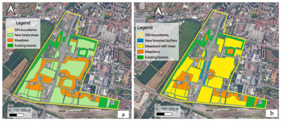
Figure 2.
Intervention scenarios and their different land uses: (a) urban forest scenario and (b) meadows with sparse trees scenario.
Table 1 reports details about different land uses and their area for each of the two scenarios.

Table 1.
Intervention scenarios and land use categories within them.
For scenario 1, it was assumed that maintenance activities will be implemented for the first three years after planting and will consist of grass cutting and irrigation on demand, to reduce the risk of mortality. Management operations will consist of two thinning rounds: a first round at year 10, removing 25 to 30% of existing trees (warped, shadowed and dominated, etc.) corresponding to an estimated harvested volume of 50–75 m3/ha; and a second round between year 30 and year 40, removing 30 to 50% of existing trees, i.e., an estimated harvested volume of 250–350 m3/ha.
2.3. Methodological Approaches for Ecosystem Service Assessment
For both scenarios, a set of nine ESs was defined in cooperation with ERSAF specialists. The selected ESs cover the three main ES sections according to the Common International Classification of Ecosystem Services (CICES) version 5.1 [86]. Specific assessment approaches were identified for each of them (Table 2). The provision of biomass and fibers for processing and energy (1.1) was assessed only in the case of scenario 1, as no forest management intervention was forecast for scenario 2; meanwhile, phytoremediation capacity (2.1) was assessed only for scenario 2 due to a lack of robust literature regarding phytoremediation capacity for the tree species planned there.
Table 2.
Overview of ecosystem services targeted by the research and assessment approaches.
As reported by Table 2, different software suites and models were used for the assessment, including InVEST 3.9.0 [87], i-Tree Eco version 6.0 [88] and ESTIMAP [89]. The selected models were specifically designed to assess most of the ESs addressed by this study, except for the provision of biomass and fibers for processing and energy, and phytoremediation capacity. Selected software suites also included models that allow for the assessment of carbon sequestration; however, they tend to be data-intensive. In these three cases, alternative methods and approaches were used. Details about data inputs and methodological aspects for each ES assessed and models/approaches adopted, including details about monetary estimations, are provided in Section 2.4 below.
For land use data, reference was made to the Regional Land use Database for Lombardy [91], integrated with specific land use data for each intervention scenario. Geospatial data were elaborated using QGIS 3.16.
ES were assessed according to the “with and without” principle [92], i.e., as a difference between values accounted under each of the two intervention scenarios and the baseline conditions. Whenever possible, the economic assessment was performed as an initial (i.e., at present time) accumulation of values, taking into consideration two different time horizons, i.e., 60 years and infinite (present value of an infinite annual series). A 3% discount rate was adopted according to the European Commission’s guidelines for investment appraisal [93].
When annual values were not directly provided as a model output, they were computed starting from present values of terminating annual series, and using the inverse formula for the computation of single annuities.
2.4. Models and Approaches Used for the Assessment: Data Inputs and Methodological Details
Within this section a description of each model/approach used for the assessment and evaluation of the selected ESs is provided, together with details about input data and their sources.
2.4.1. Provision of Biomass and Fibers for Processing and Energy
This ES was only estimated for scenario 1 by referring to expected removals from forecasted management operations (thinning and maintenance, see Section 2.2). It is assumed that biomass retrieved from management activities will only consist of assortments suitable for energy use, i.e., chipped wood from the first thinning round and firewood from the second one. Wood prices for firewood and chipped wood were collected from local Chambers of Commerce.
An overview of input and output data for this approach is reported in Table 3.
Table 3.
Input and output data for the assessment and evaluation of the provision of biomass and fibers.
The economic value of the biomass and fibers provisioning service was computed according to Equation (1):
where:
- WV = wood assortment value, EUR
- R = volume of removals per thinning round i, m3
- WD = wood density for each of the j wood species considered, kg/m3
- Wp = wood price per assortment k (either chipped wood or firewood), EUR/Mg.
WV values were discounted to present time, then converted into single annuities (a) by considering the reverse formula of a terminating annual series covering 60 years. The infinite annual series case was not considered in this case, as only two thinning rounds have been defined.
2.4.2. Phytoremediation Capacity
This ES was only estimated for scenario 2. Reference was made to specific guidelines for reclamation and phytoremediation for the SIN Brescia-Caffaro [90], and to replacement costs for alternative measures (on-site thermal treatment) that would ensure equivalent remediation performances. The economic value of the phytoremediation capacity equals the unit cost for the on-site thermal treatment multiplied by the volume of soil to be treated. Given the high variability of costs associated with alternative measures, three cost options—i.e., minimum (51 EUR/m3), average (122 EUR/m3) and maximum (194 EUR/m3)—were considered [95]. The total volume of soil to be treated corresponds to 438,600 m3, i.e., the whole contaminated area for a 1 m depth.
An overview of input and output data for the assessment and evaluation of phytoremediation capacity is reported in Table 4.
Table 4.
Input and output data for the assessment and evaluation of phytoremediation capacity.
2.4.3. Removal and Filtration of Air Pollutants
i-Tree Eco version 6.0, developed by the United States Department of Agriculture Forest Service [88], was used to assess and evaluate this ES. The pollutants considered included Ozone (O3), Nitrogen dioxide (NO2), Carbon monoxide (CO), Sulfur dioxide (SO2), and fine particles, i.e., particulate matter (PM 2.5).
The economic value of this ES was estimated in terms of avoided costs, with reference to the expected reduction in mortality and illness rates due to the reduced amount of pollutant concentration in the air. The model estimated costs based on the open-source computer program Environmental Benefits Mapping and Analysis Program—Community Edition (BenMAP-CE) [96], with reference to a target population exposed to pollution risks and, therefore, benefiting of any reduction in pollutant concentration. For this aim, the population living within a radius of 1 km around the case study area was considered the target population. This radius was assumed to be appropriate for a perceivable reduction in pollutant concentration and air quality [97].
Table 5 shows input and output data for the model.
Table 5.
Input and output data for the assessment and evaluation of removal and filtration of air pollutants.
2.4.4. Protection against Hydrogeological Risks and Control of Erosion
This ES was assessed and evaluated using the InVEST 3.9.0 Urban flood risk mitigation model [100], which calculates the runoff depth and runoff depth reduction from rainfall depth, i.e., the amount of runoff retained compared to a given precipitation volume, using the Curve Number method [101,102]. Input data for the model, as well as outputs, are shown in Table 6. The economic value of the ES was assessed via the replacement cost method, using a lamination basin as a surrogate good, assuming a unit cost of 400 EUR/m3, estimated via the Regional Law on 23rd November 2017, n. 7 of Lombardy Region (art. 16), and adjusted based on [103].
Table 6.
Input and output data for the assessment and evaluation of protection against hydrogeological risks and control of erosion.
2.4.5. Pollination
Pollination was assessed and evaluated using the InVEST 3.9.0 Pollinator Abundance: Crop Pollination model [100]. This model focuses on wild and managed pollinators and uses the availability of nest sites and floral resources within bee flight ranges to derive an index of the abundance of bees nesting. It then uses floral resources, pollinator foraging activity and flight range information to estimate an index of the abundance of pollinators, and finally, calculates a simple index of the contribution of these pollinators to agricultural production, based on their abundance and crop dependence on pollination. Based on yields per single crop type, it is therefore possible to calculate the crop yield attributable to pollinators and, using crop market prices, estimate the economic value of the pollination ES. Selected pollinator species included bumblebee, bee (miner and carpenter bee), hoverfly, ant, butterfly and wasp. Crop yields for different crop types were retrieved from the Benchmark Yield Database of the National Agriculture Information System [106], while crop prices were collected from the Chambers of Commerce of Milan and Brescia.
Input and output data for this model are reported in Table 7.
Table 7.
Input and output data for the assessment of pollination.
2.4.6. Biodiversity and Habitat Quality
This ES was assessed and evaluated via the InVEST 3.9.0 Habitat Quality Model [100], which estimates patterns in biodiversity by analyzing land use/land cover in conjunction with threats to species’ habitats. The model uses habitat quality as a proxy for biodiversity. It computes a habitat quality index (ranging between 0 and 1) as a function of four factors: each threat’s relative impact; the relative sensitivity of each habitat type to each threat; the distance between habitats and sources of threats; and the degree to which the land is legally protected [100]. For the economic evaluation, reference was made to values estimated by [109] regarding the economic loss associated with biodiversity decline due to soil consumption and urban development. Average unit values (EUR/m2) for different land use conversions/transformations were estimated, then linked to different land uses and, finally, multiplied by the corresponding habitat quality index through the raster calculator function in QGIS 3.16.
Detailed information about input and output data for this model is available in Table 8.
Table 8.
Input and output data for the assessment and evaluation of biodiversity and habitat quality.
2.4.7. Carbon Sequestration
Although selected models allow for the assessment of carbon sequestration, they tend to be data-intensive; therefore, an alternative approach based on the International Panel on Climate Change (IPCC) guidelines [112] and additional stock data from the literature [103,113] was used. For the estimation of the economic value of the ES, the estimated Carbon stock under each scenario was multiplied by an average carbon price, retrieved from existing literature on forest-based carbon-projects and initiatives in Italy [114].
Table 9 includes input and output data for the carbon sequestration model.
Table 9.
Input and output data for the assessment and evaluation of carbon sequestration.
2.4.8. Temperature Regulation and Urban Cooling
This ES was assessed and evaluated via the InVEST 3.9.0 Urban Cooling Model [100] that—based on shade, evapotranspiration, and albedo, as well as distance from cooling islands (green areas larger than 2 ha)—calculates a heat mitigation index, estimating a temperature reduction by vegetation and green spaces. The model also estimates the economic value of the ES in terms of avoided costs associated with avoided energy consumption due to the cooling effects of vegetation.
Input and output data for the temperature regulation and urban cooling model are summarized in Table 10.
Table 10.
Input and output data for the assessment of temperature regulation and urban cooling.
Based on model outputs, the Discomfort Index (DI) was calculated. This corresponds to a physiological thermal stress indicator for people, based on dry-bulb and wet-bulb temperature [121,122] according to the following:
where:
DI = 0.4 (Ta + Tw) + 4.8
- Ta = dry-bulb temperature (°C) from the InVEST Urban Cooling model
- Tw = wet-bulb temperature (°C) from the InVEST Urban Cooling model.
2.4.9. Recreation
Recreation was assessed based on an adapted version of ESTIMAP [89,123] a GIS-based model for the assessment, estimation, and mapping of ESs developed by the Joint Research Centre (JRC) of the European Commission. The model computes the Recreational Opportunity Spectrum (ROS), ranging between 0 and 1, which indicates the degree of recreation provision based on a combination of multiple natural, accessibility, and use-related features (Figure 3).

Figure 3.
Flow-chart of methodological steps for the assessment of recreation. Adapted from [89,123].
Table 11 reports input and output data for the recreation model.
Table 11.
Input and output data for the assessment and evaluation of recreation.
For the economic evaluation, the spatial distribution of potential users and the number of trips to the area were estimated through distance-decay modelling, assuming that the recreation potential decreases as the distance from a specific feature (e.g., forest area) increases [89]. The following distance decay function was adopted [89,124,125]:
where:
- d = distance in meters from the specific feature
- α and K = e size and shape parameters of the function adjusted according to a distance threshold. They were assumed to be 0.0009 and 30, respectively, corresponding to distance thresholds of 4000 m at which the score was decreased by 50%, and 8000 at which the score was zero [89]. The choice of parameter values also reflects limitations in access to the area, for instance, by making only specific paths and tracks viable, due to contamination risks.
The number of trips was attributed to the resident population [126] to calculate the outdoor recreation demand, assuming that all inhabitants in the case study area had similar desires in terms of (everyday life) outdoor recreational opportunities, but their level of fulfillment depended on proximity to recreation sites [89,125]. The population living within an 8000 m radius was considered, making reference to 300 m distance breaks [125,127]. The economic value associated to each trip was 1.44 EUR/trip, derived from previous studies within similar urban contexts [103] and adjusted via the ROS.
3. Results
This section provides the research results, distinguishing them into the assessment of single ESs (Section 3.1), and a summary of results and total value for the two intervention scenarios (Section 3.2).
3.1. Assessment of Single Ecosystem Services
3.1.1. Provision of Biomass and Fibers for Processing and Energy
For the first thinning round (year 10), removals are expected to range between 50 and 70 m3/ha, over a total area covering 30.75 ha: this corresponds, in total, to 1150.93–1611.30 Mg of chipped wood. By considering a unit price of 30.50 EUR/Mg, a total economic value between EUR 35,103.32 and 49,144.65 is estimated. When discounted to the present time, this equals EUR 26,120.17 to 36,568.24. For the second thinning round (year 35), the removed volumes range between 250 and 350 m3/ha, i.e., between 5764.64 and 8056.50 Mg of firewood in total. Assuming a unit price of 40 EUR/Mg, this corresponds to EUR 230,185.71–322,260, equivalent to discounted values ranging between EUR 81,804.18 and 114,525.85. In total, the present value expected from the two rounds of thinning falls within EUR 107,924.35 and 151,094.09, i.e., an estimated annual value between EUR 3899.63 and 5459.48.
3.1.2. Phytoremediation Capacity
It is estimated that tall fescue can remove all pollutants in 90 years, while in 60 years, 80% of the pollutants are removed [90]. Based on the three different unit cost hypotheses for alternative measures (on-site thermal treatment)—i.e., minimum, average and maximum unit cost—the estimated annual ES values range between EUR 109,749 and 417,475, with an intermediate value of EUR 262,536, and corresponding present values (over 60 years) ranging from EUR 3 million to EUR 11.5 million, with an intermediate value of about EUR 7.3 million.
3.1.3. Removal and Filtration of Air Pollutants
The two intervention scenarios show similar profiles; however biophysical and economic values for scenario 1 are about four times higher (Figure 4): the forest is estimated to remove some 2.91 Mg/year of pollutants, while for meadows with sparse trees, the estimation is approximately 0.67 Mg/year. Under both scenarios, the pollutants removed mainly consist of Ozone (O3) (61%), and Nitrogen dioxide (NO2) (31%), with lower contributions by Carbon monoxide (CO) (about 4%) and Sulfur dioxide (SO2) (3.5%), and a marginal contribution by fine particles, i.e., particulate matter (PM) 2.5 (0.5%). However, as for the economic value, while O3 still ranks first, PM2.5 follows, because it is the most health-harmful among the pollutants considered by iTree. The economic value of this ES is estimated to be 9086.84 EUR/year in the case of the urban forest and 2209.72 EUR/year in the case of meadows with sparse trees. This corresponds, respectively, to a present value of EUR 48,589.32 and EUR 11,213.33 over a 60-year-long time horizon, or EUR 100,000.57 and EUR 23,715.42 over an infinite time horizon.
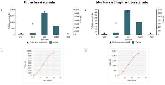
Figure 4.
Total pollution removed and economic value of the ES per year and per pollutant (a,c), and total value variation over time (b,d) under the two intervention scenarios. Please note that the charts use different scales on the vertical axes.
3.1.4. Protection against Hydrogeological Risks and Control of Erosion
The runoff retention results are higher for scenario 1 than for scenario 2 under all the rainfall depth values (h) and return time conditions considered (Figure 5). For scenario 1, the runoff retention ranges between 20,949 m3 (equivalent to 0.021 m3/m2)—for an h value of 26.4 mm—and 34,400 m3—for an h value of 55.9 mm (0.035 m3/m2), with an intermediate volume of 28,877 (0.030 m3/m2) for an h value of 41.8 mm. For scenario 2 the runoff retention varies between 20,289 m3 (0.021 m3/m2) for h equal to 26.4 mm and 32,250 m3 (0.033 m3/m2) for h equal to 55.9 mm, with an intermediate value of 27,454 m3 (0.028 m3/m2) for h equal to 41.8 mm.
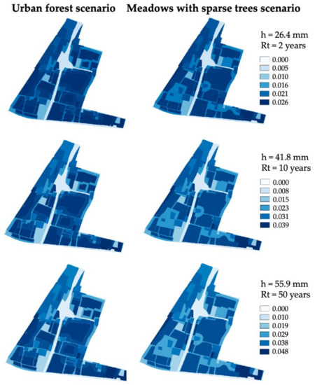
Figure 5.
Runoff retention (m3) for the baseline and the two intervention scenarios under different depth of rainfall (h, mm) and return time conditions (Rt, years).
The modelled biophysical values reflect economic ones: annual values estimated for this ES range between 40,423 and 111,432 EUR/year for scenario 1 (intermediate value: 80,061 EUR/year), and between 30,882 and 81,789 EUR/year for scenario 2 (intermediate value: 59,488 EUR/year). For scenario 1, the present values fall within EUR 1.12 and 3.08 million (over a 60-year-long time horizon) and EUR 1.35 and 3.71 million (infinite time horizon). For scenario 2, they range between EUR 0.85 and 2.26 million (over a 60-year-long time horizon) and between EUR 1.03 and 2.73 million (over an infinite time horizon).
3.1.5. Pollination
Both intervention scenarios result in improved habitat for pollinators and, therefore, in better conditions for their abundance and activities; these ultimately have effects on the economic value of the ES in terms of the production of pollinator-dependent crops. This corresponds to annual values estimated to be 6200.56 EUR/year for scenario 1 and 5436.50 EUR/year for scenario 2. The present value for 60 of these annuities corresponds to EUR 171,603.92 and EUR 150,458.16, respectively, while the present value when considering an infinite time horizon corresponds to EUR 206,685.25 and EUR 181,216.62, respectively.
3.1.6. Biodiversity and Habitat Quality
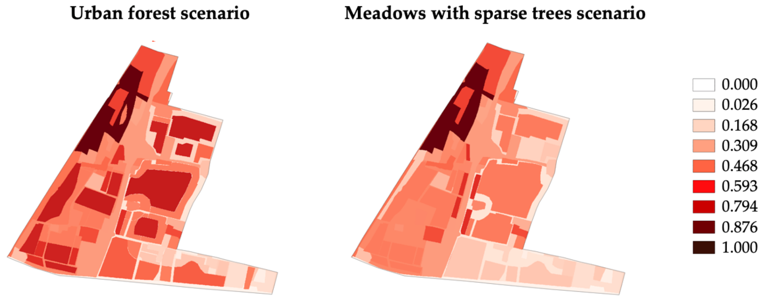
The habitat quality index varies greatly under both scenarios (Figure 6), showing the highest values for land use categories such as riparian woods, broadleaf high forests, and permanent meadows with and without trees and shrubs. The average value of the index is highly influenced by the relative abundance of the most valuable land uses and habitats, with scenario 1 showing a higher value than scenario 2 (0.609 vs. 0.549). This reflects the economic values; the annual value for the urban forest corresponds to EUR 12,024.87 and for the meadows with sparse trees, 5836.46 EUR. The accumulation, up to the present time, of 60 of these annuities is equal to EUR 0.41 million and EUR 0.24 million, respectively. The present value, when considering an infinite time, is equal to to EUR 0.49 million and EUR 0.29 million.
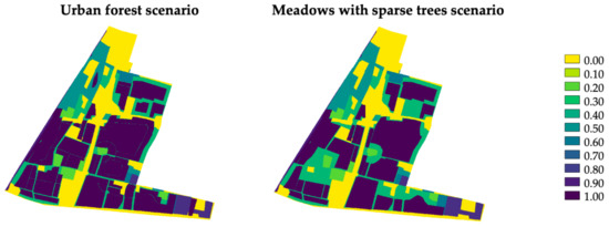
Figure 6.
Habitat quality index for the two intervention scenarios.
3.1.7. Carbon Sequestration
Scenario 1 shows better performances in terms of carbon sequestration, with an estimated stock of 11,724.63 MgCO2 (91% due to the forest stand and the rest to the meadows), i.e., more than 1.8 times the stock estimated for scenario 2 (6376.72 MgCO2). As for the latter, the main pools are soil (about 47%) and standing trees (40%). In the case of soil, reference was made to the stock at the 60th year rather than considering an annual increment. Assuming a unit price of 10.68 EUR/Mg of CO2eq [114], an annual value of EUR 2473.85 was estimated for scenario 1 and EUR 471.62 for scenario 2. This corresponds, respectively, to present values of EUR 19,309.04 and EUR 6152.90 (over a 60-year-long time horizon), and EUR 82,461.56 and EUR 15,720.59 (over an infinite time horizon).
3.1.8. Temperature Regulation and Urban Cooling
The heat mitigation index shows a decreasing trend when moving from the core of the case study area to more marginal areas, particularly when moving northeast (Figure 7). The index varies within similar ranges (0.020–0.837) for the two intervention scenarios; however, the average value is higher for scenario 1 (0.404) than for scenario 2 (0.394). This reflects the expected average air temperature within buildings in the area: 24.45 °C for scenario 1 and 25.49 °C for scenario 2. The dry- and wet-bulb temperatures estimated by the model were used for the calculation of the Discomfort Index [121,122]; in both cases, it is below 24 °C (23.86 °C for scenario 1 and 23.89 °C for scenario 2) which, according to [121], means that less than 50% of the population in the area feels discomfort. Notably the same index computed for the baseline situation is 26.06 °C, implying that more than 50% of the population feels discomfort [121].
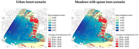
Figure 7.
Heat mitigation index and average air temperature (°C) for the two intervention scenarios.
The cooling effect of the urban forest is estimated to save 219.04 EUR/day in terms of energy savings for the buildings within a 200 m-wide buffer around the case study area. Assuming that there are 73.5 summer days/year [128], this corresponds to 16,099 EUR/year. The present value, when considering 60 annuities, would correspond to EUR 445,561, while the present value, over an infinite time horizon, would be EUR 536,648. In the case of the meadows with sparse trees, the estimated daily savings are 213.17 EUR/day, corresponding to 15,668 EUR/year. The initial accumulation over sixty years would lead to a total value of EUR 433,621, while the present value over an infinite time would be EUR 522,267.
3.1.9. Recreation
The Recreational Opportunity Spectrum (ROS) varies across the site and depending on the scenario. It shows an average value that is higher for scenario 1 (0.371) than for scenario 2 (0.351) (Figure 8). When focusing just on the areas subject to land use change under the two scenarios:
- In scenario 1, new forest areas show a ROS ranging between 0.415 and 0.7, with an average value of 0.608, while meadows associated with them have a ROS ranging between 0.213 and 0.674, with an average score of 0.42.
- In scenario 2, the new meadows show a ROS ranging between 0.213 and 0.622, with an average value of 0.419.

Figure 8.
Recreation Opportunities Spectrum for the two intervention scenarios.
Figure 8.
Recreation Opportunities Spectrum for the two intervention scenarios.
The expected number of visits per year is 59,251 for scenario 1 and 56,316 for scenario 2; this corresponds to annual economic values of, EUR 31,654 and EUR 28,464, respectively (i.e., about 8555 EUR/year and 5365 EUR/year higher than the values estimated for the baseline). The present value of these annuities over 60 years corresponds to EUR 236,764.45 and EUR 148,479.40, respectively, while the initial accumulation in the case of an infinite time is EUR 178,883.33 and EUR 948,808.72.
3.2. Summary of Results and Total Value for the Intervention Scenarios
A summary of the estimated values for all ESs considered within this research is provided in Table 12 for scenario 1, and in Table 13 for scenario 2. The relative sharing of ES values under the two scenarios is reported in Figure 9.
Table 12.
Summary of ES values for scenario 1—urban forest.
Table 13.
Summary of ES values for scenario 2—meadows with sparse trees.

Figure 9.
Relative sharing of ES values in terms of annual flow, present value over 60 years and an infinite time horizon for the two intervention scenarios. (a) Scenario 1—Urban forest, (b) Scenario 2—Meadows with sparse trees.
Both intervention scenarios show ES values that exceed the baseline, thus indicating substantial improvements associated with NBS development. When considering a single ES, scenario 1 systematically performs better than scenario 2, with the only exception being the phytoremediation capacity, which is not considered in the case of the urban forest. When considering the total value for the full set of ESs taken into account, scenario 2 shows the highest value, mainly due to the contribution of the phytoremediation capacity. The total annual flow values estimated are 139,181 EUR/year for scenario 1 and 357,011 EUR/year for scenario 2, equivalent to 0.42 EUR/year m2 and 0.82 EUR/year m2, respectively, and to 0.70 EUR/year and 1.79 EUR/year per single inhabitant living within Brescia municipality. When considering the ES stocks instead of their annual flows, the estimated economic value for the stock over a 60-year period is EUR 3.60 million for scenario 1 (10.81 EUR/m2) and EUR 9.83 million for scenario 2 (22.05 EUR/m2). When an infinite time horizon is considered, the total present value of the stock amounts to EUR 4.28 million for scenario 1 (12.84 EUR/m2) and EUR 3.10 million for scenario 2 (6.85 EUR/m2). As for the latter, the values are influenced by the fact that the stock value for the phytoremediation capacity ES is not considered under an infinite time horizon, as the remediation action would terminate in 90 years.
Note: scenario 1 does not include phytoremediation capacity, and scenario 2 does not include the provision of biomass and fibers for processing and energy. In scenario 2 phytoremediation is not accounted for in the case of infinite time.
Under both scenarios, a single ES dominates the total value, with remaining ESs contributing to different extents (Figure 9):
- For scenario 1, more than half of the value (57–62%) is attached to the protection against hydrogeological risks and control of erosion, followed by temperature regulation and urban cooling (12–13%); biodiversity and habitat quality (9%); recreation (6–7%); and pollination (4–5%). Altogether these ESs account, on average, for more than 93% of the total value estimated for the urban forest scenario, while other ESs contribute marginally.
- For scenario 2, phytoremediation capacity is the leading ES (74%), followed by the protection against hydrogeological risks and control of erosion (17%); temperature regulation and urban cooling (4%); pollination; biodiversity and habitat quality; and recreation (2–6% each). When an infinite time horizon is considered, the contribution of phytoremediation capacity is not accounted for; the protection against hydrogeological risks and control of erosion becomes the main ES (64%), and temperature regulation and urban cooling grows up to a 17% contribution.
4. Discussion
Research results show that both brownfield redevelopment scenarios are expected to create urban green spaces, generating a wide range of ESs to an extent that goes far beyond the level of ESs provided under the current conditions. This confirms existing literature on this topic [129], according to which NBSs have the potential to supply multiple ESs and offer opportunities that are beneficial to a vast range of people [67,68]. In particular, urban NBSs often provide local public goods [130], primarily benefitting citizens in the area in which they are located [64].
Regulating ESs contribute the most to the overall estimated ES value; this is, on the one hand, consistent with findings in the literature [15,131], and on the other, very much dependent on the selected set of ESs. The marginal role of provisioning ESs depends on the rationale and general logic behind the two intervention scenarios that, being designed from a public perspective, are not aimed at commodity production; rather, they are aimed at the delivery of benefits to society at large. Moreover, provisioning and, to a lower extent, cultural ESs are subject to the restrictions imposed on current limitations in terms of use of, and access to, the area. All in all, this favors indirect-use values embodied within regulating ESs.
Two regulating ESs largely prevail in terms of value under the two scenarios: phytoremediation capacity, and protection against hydrogeological risks and control of erosion. The latter is functionally linked to the former, as it can be assumed that by improving runoff retention capacity, the transport of polluted soil and sediments towards downstream areas and water bodies, including groundwater, can be reduced [132]. It should not be forgotten that due to the lack of systematic data on phytoremediation projects using trees in urban areas, the phytoremediation capacity was not assessed for scenario 1. However, existing literature indicates that several tree species, including some of those planned to be planted in the new urban forest (e.g., Quercus robur, Carpinus betulus etc.), have phytoremediation potential and the capacity to withstand stress by pollutants and heavy metals [133]. The total value of ESs delivered under scenario 1 is, therefore, likely to be underestimated, and the gap among the two scenarios is probably narrower. The fact that phytoremediation capacity and protection against hydrogeological risks and control of erosion largely prevail in terms of estimated value does not mean that other ESs delivered by the two scenarios are negligible. This is particularly evident for scenario 1, wherein, besides protection against hydrogeological risks and control of erosion, another six ES make about 40% of the total estimated value.
Further underestimation of ESs is also due to the fact that this study does not consider the full range of potential ESs that could be delivered by the two intervention scenarios; rather, it focuses on a set of ESs selected a priori. While the selected set includes the most plausible ESs given the expected transformation projects, they still exclude some ESs (e.g., landscape and aesthetics, and other cultural services, such as those falling within the g domain of green care initiatives [134] for physical and psycho–social wellbeing) that could bring in additional value. In addition to this, the study does not aim to grasp the total economic value (TEV) of the two intervention scenarios, and some TEV components—in particular, those associated to non-use values—are, therefore, not considered and accounted for.
Notwithstanding the many barriers and challenges, brownfield redevelopment is of relevance due to the processes of de-industrialization and suburbanization, as well as population resettlement occurring within and around urban areas [135]. Within existing settlements, particularly dense ones, there may be limited room for developing additional green spaces; therefore, brownfields could provide opportunities for this [21]. Redeveloped brownfields and green urban brownfields can become vital components of a city’s green infrastructure, being connected with, and complementing a wide variety of green features within urban settlements, as well as supporting the connection of urban and rural areas [136]. If properly planned as a mix of developed and green areas, they may be part of an effective strategy to tackle or mitigate land consumption and urban sprawl processes, while at the same time improving quality of urban areas. Ideally, brownfields give opportunities to exploit large sources of land within established communities, often offering already excellent infrastructure [137]. Nevertheless, investors still prefer new locations when investing in development projects, targeting undeveloped land (“greenfields”) that are free of many risks and uncertainties associated with brownfields [138]. This, ultimately, may result in increased land consumption and urban sprawl [139]. Brescia makes no exception in this regard, ranking second among municipalities in Lombardy and among provinces at the national level in terms of total annual land consumption [140]; greenfield sites are being developed, while large brownfields, such as the SIN Caffaro, have remained vacant for decades. The implementation of effective NBSs can be strategic in brownfield redevelopment and the valuing of green urban brownfields, thus contributing to solving a dual land-use policy challenge (reducing the barriers to private-sector redevelopment, for instance, by having positive spillover effects on property values [141,142], while connecting reuse to broader community goals [137]). Despite recent progress and advancements in characterizing the benefits of NBSs and green infrastructure within the academic community [143], it remains challenging for decision makers to incorporate their benefits into urban design and planning [56,71]. Barriers include the need to better embody these concepts within the existing policy mix, providing technical support via trials and best practices, defining appropriate economic mechanisms, and setting effective institutional and governance frameworks [12,14]. This also implies the consideration of innovative financial mechanisms for the development of NBSs and support of their implementation in practice, as a recurring key barrier is obtaining finance, whether public or private [10,12,64]. While NBS could, in principle, be framed within the urban infrastructure domain that traditionally falls within public investments, rapid urbanization and a lack of public funding for urban NBSs may render the involvement of private investors attractive, and sometimes even necessary [64,144]. There are a lot of instruments that local governments can explore to leverage private sources’ involvement [145]. Gathering robust data on the benefits delivered by NBSs, including monetary values, is key to informing public decision making on innovative solutions aimed to deliver public goods while attracting potential investors, thus enabling the sharing of costs and risks associated with long-term investments [146], and favoring efficiency while delivering ESs [147].
5. Conclusions
In this study, we estimated—both in biophysical and monetary terms—expected ESs under alternative NBS-based intervention scenarios for the redevelopment and valuing of an urban brownfield within the municipality of Brescia, Northern Italy. Results show that both scenarios improve the ES stock and flows compared to the baseline, thus ensuring a broad range of benefits to local communities. Scenario 1 shows higher values when single ESs are considered, while scenario 2 shows higher total values, as it also accounts for the phytoremediation capacity ES that is not considered under the first scenario. All in all, regulating ESs represent the bulk of estimated ESs, thus highlighting the potential of proposed NBS solutions for improving urban resilience vis-à-vis existing challenges—such as those posed by the management of a contaminated site, or climate-change-related hazards (e.g., flood risks, rising temperatures, and the urban heat-island effect)—while also considering the increasing societal demand for green spaces within urban settlements.
Although the potential of NBSs as a cost-effective enabler of urban sustainability has been recognized, the implementation, management, and upscaling of NBSs face numerous barriers and challenges. The effective assessment of benefits delivered by urban NBSs represents one of them. The ES assessment and valuation exercise presented within this paper is an example of how research and practice can be integrated to inform urban management activities and provide inputs for future decision making and planning regarding urban developments. The results confirm that existing models and approaches for ES valuation can be effectively used for valuing NBSs, thus contributing to research and practice in setting up a standardized framework for a quick and effective assessment of urban NBSs, both in biophysical and monetary terms.
Despite our efforts, the paper has some limitations. The first includes the a priori selection of ESs and the TEV components targeted by the research, which likely resulted in underestimation of the total value of ESs generated by NBSs under the two intervention scenarios. Future research might aim to enlarge the scope of ESs covered, for instance, by also including phytoremediation capacity in the case of forest projects. A second limitation derives from the combination of traditional estimation approaches and software-based models that required some simplifications or assumptions in modeling, due to technical constraints or data gaps in terms of quality/scale and quantity.
This research is focused on ES supply and does not take into consideration ES demand by potential beneficiaries, which could be explored in future studies. This would allow an exploration of stakeholders’ needs and preferences, providing additional inputs for setting priorities in decision-making and planning activities associated with NBS development, as well as in detecting willingness to pay for the benefits generated.
Author Contributions
Conceptualization, M.M., A.B., G.A. and F.M.; methodology, M.M., G.A. and F.M.; software, M.M., A.B. and G.A.; validation, M.M., G.A., P.N. and S.A.; formal analysis, M.M., A.B., G.A. and F.M.; investigation, M.M., A.B., G.A. and F.M.; data curation, M.M., A.B., G.A., F.M., P.N. and S.A.; writing—original draft preparation, M.M.; writing—review and editing, M.M., A.B., G.A., F.M., D.P., P.N. and S.A.; visualization, M.M., A.B., G.A., F.M., D.P., P.N. and S.A.; supervision, M.M.; funding acquisition, M.M. and P.N. All authors have read and agreed to the published version of the manuscript.
Funding
This research was funded by ERSAF under agreement 2020_5726.
Institutional Review Board Statement
Not applicable.
Informed Consent Statement
Not applicable.
Data Availability Statement
Not applicable.
Acknowledgments
We would like to acknowledge the ERSAF staff for supporting the research by providing access to the data. We are grateful to the two anonymous reviewers for their insightful revision suggestions.
Conflicts of Interest
The authors declare no conflict of interest. The ERSAF staff were involved in the design of alternative scenarios, facilitating access to the data needed as inputs for the study, and reviewing results.
References
- UNFPA. United Nations Population Fund. Available online: https://www.unfpa.org/urbanization (accessed on 10 December 2021).
- Borelli, S.; Conigliano, M.; Pineda, F. Unasylva 250; FAO: Rome, Italy, 2018; Volume 69, pp. 3–10. [Google Scholar]
- Aurambout, J.P.; Schiavina, M.; Melchiori, M.; Fioretti, C.; Guzzo, F.; Vandecasteele, I.; Proietti, P.; Kavalov, B.; Panella, F.; Koukoufikis, G. Shrinking Cities—JRC126011; European Commission: Brussels, Belgium, 2021. [Google Scholar]
- Kabisch, N.; Korn, H.; Stadler, J.; Bonn, A. Nature-Based Solutions to Climate Change Adaptation in Urban Areas: Linkages between Science, Policy and Practice; Springer: Cham, Switzerland, 2017. [Google Scholar]
- Vardoulakis, S.; Kinney, P. Grand Challenges in Sustainable Cities and Health. Front. Sustain. Cities 2019, 12, 1–7. [Google Scholar] [CrossRef] [Green Version]
- UN. Transforming Our World: The 2030 Agenda for Sustainable Development; United Nations: New York, NY, USA, 2015. [Google Scholar]
- World Forum on Urban Forests. Greener, Healthier and Happier Cities for All—A Call for Action. In Proceedings of the World Forum on Urban Forests, Mantova, Italy, 27 November–1 December 2018. [Google Scholar]
- United Nations Human Settlements Programme. The New Urban Agenda; United Nations Human Settlements Programme: Nairobi, Kenya, 2020. [Google Scholar]
- Dorst, H.; van der Jagt, A.; Raven, R.; Runhaar, H. Urban Greening through Nature-Based Solutions—Key Characteristics of an Emerging Concept. Sustain. Cities Soc. 2019, 49, 101620. [Google Scholar] [CrossRef]
- Davies, C.; Lafortezza, R. Transitional Path to the Adoption of Nature-Based Solutions. Land Use Policy 2019, 80, 406–409. [Google Scholar] [CrossRef]
- Dorst, H.; van der Jagt, A.; Raven, R.; Runhaar, H. Structural Conditions for the Wider Uptake of Urban Nature-Based Solutions—A Conceptual Framework. Cities 2021, 116, 103283. [Google Scholar] [CrossRef]
- Nesshöver, C.; Assmuth, T.; Irvine, K.N.; Rusch, G.M.; Waylen, K.A.; Delbaere, B.; Haase, D.; Jones-Walters, L.; Keune, H.; Kovacs, E.; et al. The Science, Policy and Practice of Nature-Based Solutions: An Interdisciplinary Perspective. Sci. Total Environ. 2017, 579, 1215–1227. [Google Scholar] [CrossRef]
- Sowińska-Świerkosz, B.; García, J. What Are Nature-Based Solutions (NBS)? Setting Core Ideas for Concept Clarification. Nature-Based Solut. 2022, 2, 100009. [Google Scholar] [CrossRef]
- Maes, J.; Jacobs, S. Nature-Based Solutions for Europe’s Sustainable Development. Conserv. Lett. 2015, 10, 121–124. [Google Scholar] [CrossRef] [Green Version]
- Gómez-Baggethun, E.; Barton, D.N. Classifying and Valuing Ecosystem Services for Urban Planning. Ecol. Econ. 2013, 86, 235–245. [Google Scholar] [CrossRef]
- Frantzeskaki, N.; Kabisch, N.; McPhearson, T. Advancing Urban Environmental Governance: Understanding Theories, Practices and Processes Shaping Urban Sustainability and Resilience. Environ. Sci. Pol. 2016, 62, 1–6. [Google Scholar] [CrossRef]
- Potschin-Young, M.; Haines-Young, R.; Görg, C.; Heink, U.; Jax, K.; Schleyerb, C. Understanding the Role of Conceptual Frameworks: Reading the Ecosystem Service Cascade. Ecosyst. Serv. 2018, 29 (Pt C), 418–440. [Google Scholar] [CrossRef]
- Potschin, M.; Haines-Young, R. Defining and Measuring Ecosystem Services. In Routledge Handdbook of Ecosystem Services; Potschin, M., Haines-Young, R., Fish, R., Turner, R.K., Eds.; Routledge: New York, NY, USA, 2016; pp. 25–44. [Google Scholar]
- Paya Perez, A.; Van Liedekerke, M.; Pelaez Sanchez, S. Remediated Sites and Brownfields. Success Stories in Europe; European Commission: Brussels, Belgium, 2015. [Google Scholar]
- Raymond, C.M.; Frantzeskaki, N.; Kabish, N.; Berry, P.; Breil, M.; Nita, M.R.; Geneletti, D.; Calfapietra, C. A Framework for Assessing and Implementing the Co-Benefits of Nature-Based Solutions in Urban Areas. Environ. Sci. Pol. 2017, 77, 15–24. [Google Scholar] [CrossRef]
- Mathey, J.; Rößler, S.; Banse, J.; Lehmann, I. Brownfields As an Element of Green Infrastructure for Implementing Ecosystem Services into Urban Areas. J. Urban Plan. Dev. 2015, 141, A4015001. [Google Scholar] [CrossRef]
- Pueffel, C.; Haase, D.; Priess, J.A. Mapping Ecosystem Services on Brownfields in Leipzig, Germany. Ecosyst. Serv. 2018, 30, 73–85. [Google Scholar] [CrossRef]
- Hou, D.; Al-Tabbaa, A. Sustainability: A New Imperative in Contaminated Land Remediation. Environ. Sci. Pol. 2014, 39, 25–34. [Google Scholar] [CrossRef]
- O’Connor, D.; Hou, D. Targeting Cleanups towards a More Sustainable Future. Env. Sci. Process. Impacts 2018, 20, 266–269. [Google Scholar] [CrossRef]
- Song, Y.; Kirkwood, N.; Maksimović, C.; Zheng, X.; O’Connor, D.; Jin, Y.; Hou, D. Nature Based Solutions for Contaminated Land Remediation and Brownfield Redevelopment in Cities: A Review. Sci. Total Environ. 2019, 663, 568–579. [Google Scholar] [CrossRef]
- USEPA. Green Remediation: Incorporating Sustainable Environmental Practices into Remediation of Contaminated Sites; EPA 542-R-08-002; United States Environmental Protection Agency: Washington, DC, USA, 2008.
- Donaldson, R.; Lord, R. Can Brownfield Land Be Reused for Ground Source Heating to Alleviate Fuel Poverty? Renew. Energy 2018, 116, 344–355. [Google Scholar] [CrossRef] [Green Version]
- Jin, Y.; O’Connor, D.; Ok, Y.S.; Tsang, D.C.W.; Liu, A.; Hou, D. Assessment of Sources of Heavy Metals in Soil and Dust at Children’s Playgrounds in Beijing Using GIS and Multivariate Statistical Analysis. Environ. Int. 2019, 124, 320–328. [Google Scholar] [CrossRef]
- Peng, T.; O’Connor, D.; Zhao, B.; Jin, Y.; Zhang, Y.; Tian, L.; Zheng, N.; Li, X.; Hou, D. Spatial Distribution of Lead Contamination in Soil and Equipment Dust at Children’s Playgrounds in Beijing, China. Environ. Pollut. 2019, 245, 363–370. [Google Scholar] [CrossRef]
- Zhang, Y.; Hou, D.; O’Connor, D.; Shen, Z.; Shi, P.; Ok, Y.S.; Tsang, D.C.W.; Wen, Y.; Luo, M. Lead Contamination in Chinese Surface Soils: Source Identification, Spatial-Temporal Distribution and Associated Health Risks. Crit. Rev. Environ. Sci. Technol. 2019, 49, 1386–1423. [Google Scholar] [CrossRef]
- Hou, D.; O’Connor, D.; Igalavithana, A.D.; Alessi, D.S.; Luo, J.; Tsang, D.C.W.; Sparks, D.L.; Yamauchi YRinklebe, J.; Ok, Y.S. Metal Contamination and Bioremediation of Agricultural Soils for Food Safety and Sustainability. Nat. Rev. Earth Environ. 2020, 1, 366–381. [Google Scholar] [CrossRef]
- Nassuer, J.I.; Raskin, J. Urban Vacancy and Land Use Legacies: A Frontier for Urban Ecological Research, Design, and Planning. Landsc. Urban Plan. 2014, 125, 245–253. [Google Scholar] [CrossRef]
- Collier, M.J. Novel Ecosystems and the Emergence of Cultural Ecosystem Services. Ecosyst. Serv. 2014, 9, 166–169. [Google Scholar] [CrossRef] [Green Version]
- McPhearson, T.; Kremer, P.; Hamstead, Z. Mapping Ecosystem Services in New York City: Applying a Social–Ecological Approach in Urban Vacant Land. Ecosyst. Serv. 2013, 5, 11–26. [Google Scholar] [CrossRef]
- de Vries, S.; Verheij, R.A.; Groenewegen, P.P.; Spreeuwenberg, P. Natural Environments—Healthy Environments? An Exploratory Analysis of the Relationship between Greenspace and Health. Environ. Plan. A 2003, 35, 1717–1731. [Google Scholar] [CrossRef] [Green Version]
- Rodríguez-Seijo, A.; Andrade, M.L.; Vega, F.A. Origin and Spatial Distribution of Metals in Urban Soils. J. Soils Sediments 2017, 17, 1514–1526. [Google Scholar] [CrossRef]
- Brown, C.; Burns, A.; Arnell, A. A Conceptual Framework for Integrated Ecosystem Assessment. One Ecosyst. 2018, 3, e25482. [Google Scholar] [CrossRef]
- Liu, H.Y.; Jay, M.; Chen, X. The Role of Nature-Based Solutions for Improving Environmental Quality, Health and Well-Being. Sustainability 2021, 13, 10950. [Google Scholar] [CrossRef]
- Faivre, N.; Fritz, M.; Freitas, T.; de Boissezon, B.; Vandewoestijne, S. Nature-Based Solutions in the EU: Innovating with Nature to Address Social, Economic and Environmental Challenges. Env. Res. 2017, 159, 509–518. [Google Scholar] [CrossRef]
- Van den Bosch, M.; Ode Sang, Å. Urban Natural Environments as Nature-Based Solutions for Improved Public Health—A Systematic Review of Reviews. Env. Res. 2017, 158, 373–384. [Google Scholar] [CrossRef]
- Hansmann, R.; Hug, S.M.; Seeland, K. Restoration and Stress Relief through Physical Activities in Forests and Parks. Urban For. Urban Green. 2007, 6, 213–225. [Google Scholar] [CrossRef]
- Cervinka, R.; Holtgate, J.; Pirgie, L.; Schwab, M.; Sudkamp, J.; Haluza, D.; Arnberger, A.; Eder, R.; Ebenberger, M. Green Public Health—Benefits of Woodlands on Human Health and Well-Being; Bundesforschungszentrum für Wal (BFW): Vienna, Austria, 2014; ISBN 978-3-902762-32-0. [Google Scholar]
- Houlden, V.; Weich, S.; Porto de Albuquerque, J.; Jarvis, S.; Rees, K. The Relationship between Greenspace and the Mental Wellbeing of Adults: A Systematic Review. PLoS ONE 2018, 13, e0203000. [Google Scholar] [CrossRef] [Green Version]
- De Sousa, C.A. The Greening of Brownfields in American Cities. J. Environ. Plan. Manag. 2004, 47, 579–600. [Google Scholar] [CrossRef]
- Özgüner, H.; Kendle, A.D. Public Attitudes towards Naturalistic versus Designed Landscapes in the City of Sheffield (UK). Landsc. Urban Plan. 2006, 74, 139–157. [Google Scholar] [CrossRef]
- Swanwick, C. Society’s Attitudes to and Preferences for Land and Landscape. Land Use Policy 2009, 26S, S62–S75. [Google Scholar] [CrossRef]
- Mitchell, R.J.; Richardson, E.A.; Shortt, N.K.; Pearce, J.R. Neighborhood Environments and Socioeconomic Inequalities in Mental Well-Being. Am. J. Prev. Med. 2015, 49, 80–84. [Google Scholar] [CrossRef] [PubMed]
- Abhijith, K.; Kumar, P.; Gallagher, J.; Mcnabola, A.; Baldauf, R.; Pilla, F.; Broderick, B.; Di Sabatino, S.; Pulvirenti, B. Air Pollution Abatement Performances of Green Infrastructure in Open Road and Built-up Street Canyon Environments—A Review. Atmos. Environ. 2017, 162, 71–86. [Google Scholar] [CrossRef]
- Bartesaghi Koc, C.; Osmond, P.; Peters, A. Evaluating the Cooling Effect of Green Infrastructure: A Systematic Review of Methods, Indicators and Data Sources. Sol. Energy 2018, 166, 486–508. [Google Scholar] [CrossRef]
- Zardo, L.; Geneltti, D.; Pèrez-Soba, M.; Van Eupen, M. Estimating the Cooling Capacity of Green Infrastructures to Support Urban Planning. Ecosyst. Serv. 2017, 26, 225–235. [Google Scholar] [CrossRef]
- Aram, F.; Higueras Garcìa, E.; Solgi, E.; Mansournia, S. Urban Green Space Cooling Effect in Cities. Heliyon Energy 2019, 5, e01339. [Google Scholar] [CrossRef] [Green Version]
- Bolund, P.; Hunhammar, S. Ecosystem Services in Urban Areas. Ecol. Econ. 1999, 29, 293–301. [Google Scholar] [CrossRef]
- van Renterghem, T.; Attenborough, M.M.; Defrance, J.; Horoshenkov, K.; Bashirk, J.K.I.; Taherzadeh, S.; Altreuther, B.; Khan, A.; Smyrnova, Y.; Yang, H.S. Measured Light Vehicle Noise Reduction by Hedges. J. Appl. Acoust. 2014, 78, 19–27. [Google Scholar] [CrossRef] [Green Version]
- Nika, C.E.; Gusmaroli, L.; Ghafourian, M.; Atanasova, N.; Buttiglieri, G.; Katsou, E. Nature-Based Solutions as Enablers of Circularity in Water Systems: A Review on Assessment Methodologies, Tools and Indicators. Water Res. 2020, 183, 115988. [Google Scholar] [CrossRef]
- Boano, F.; Caruso, A.; Costamagna, E.; Ridolfi, L.; Fiore, S.; Demichelis, F.; Galvao, A.; Pisoeiro, J.; Rizzo, A.; Masi, F. A Review of Nature-Based Solutions for Greywater Treatment: Applications, Hydraulic Design, and Environmental Benefits. Sci. Total Environ. 2020, 711, 134731. [Google Scholar] [CrossRef] [PubMed]
- Kabisch, N.; Frantzeskaki, N.; Pauleit, S.; Naumann, S.; Davis, M.; Artmann, M.; Haase, D.; Knapp, S.; Korn, H.; Stadler, J.; et al. Nature-Based Solutions to Climate Change Mitigation and Adaptation in Urban Areas: Perspectives on Indicators, Knowledge Gaps, Barriers, and Opportunities for Action. Ecol. Soc. 2016, 21, 39. [Google Scholar] [CrossRef] [Green Version]
- Lavorel, S.; Locatelli, B.; Colloff, M.J.; Bruley, E. Co-Producing Ecosystem Services for Adapting to Climate Change. Philos. Trans. R. Soc. Lond. B Biol. Sci. 2020, 375, 20190119. [Google Scholar] [CrossRef] [PubMed] [Green Version]
- Parker, J.; Simpson, G.; Miller, J. Nature-Based Solutions Forming Urban Intervention Approaches to Anthropogenic Climate Change: A Quantitative Literature Review. Sustainability 2020, 12, 7439. [Google Scholar] [CrossRef]
- Hutchins, M.G.; Fletcher, D.; Hagen-Zanker, A.; Jia, H.; Jones, L.; Li, H.; Loiselle, S.; Miller, J.; Reis, S.; Seifert-Dähnn, I. Why Scale Is Vital to Plan Optimal Nature-Based Solutions for Resilient Citie. Environ. Res. Lett. 2021, 16, 044008. [Google Scholar] [CrossRef]
- McPhearson, T.; Andersson, E.; Elmqvist, T.; Frantzeskaki, N. Resilience of and through Urban Ecosystem Services. Ecosyst. Serv. 2015, 12, 152–156. [Google Scholar] [CrossRef]
- Dagenhart, R.; Leigh, N.G.; Skach, J. Brownfields And Urban Design: Learning From Atlantic Station. In Brownfields III. Prevention, Assessment, Rehabilitation and Development of Brownfield Site; Brebbia, C.A., Mander, U., Eds.; WIT Press: Southampton, UK, 2006; ISBN 978-1-84564-041-5. [Google Scholar]
- EC. Towards an EU Research and Innovation Policy Agenda for Nature-Based Solutions & Re-Naturing Cities; European Commission: Brussels, Belgium, 2015. [Google Scholar]
- Terton, A. Building a Climate-Resilient City: Urban Ecosystems; IISD: Winnipeg, MB, Canada, 2017. [Google Scholar]
- Toxopeus, H.; Polzin, F. Reviewing Financing Barriers and Strategies for Urban Nature-Based Solutions. J. Environ. Manag. 2021, 289, 112371. [Google Scholar] [CrossRef]
- Kumar, P.; Esen, S.E.; Yashiro, M. Linking Ecosystem Services to Strategic Environmental Assessment in Development Policies. Environ. Impact. Assess. Rev. 2013, 40, 75–81. [Google Scholar] [CrossRef]
- Croci, E.; Lucchitta, B.; Penati, T. Valuing Ecosystem Services at the Urban Level: A Critical Review. Sustainability 2021, 13, 1129. [Google Scholar] [CrossRef]
- Haase, D.; Larondelle, N.; Andersson, E.; Artmann, M.; Borgström, S.; Breuste, J.; Gomez-Baggethun, E.; Gren, Å.; Hamstead, Z.; Hansen, R.; et al. A Quantitative Review of Urban Ecosystem Service Assessments: Concepts, Models, and Implementation. Ambio 2014, 43, 413–433. [Google Scholar] [CrossRef] [PubMed] [Green Version]
- Luederitz, C.; Brink, E.; Gralla, F.; Hermelingmeier, V.; Meyer, M.; Niven, L.; Panzer, L.; Partelow, S.; Rau, A.-R.; Sasaki, R.; et al. A Review of Urban Ecosystem Services: Six Key Challenges for Future Research. Ecosyst. Serv. 2015, 14, 98–112. [Google Scholar] [CrossRef] [Green Version]
- Keyzer, M.; Sonneveld, B.; Veen, W. Valuation of Natural Resources: Efficiency and Equity. Dev. Pr. 2009, 19, 233–239. [Google Scholar] [CrossRef]
- Barton, D.N.; Kelemen, E.; Dick, J.; Martin-Lopez, B.; Gómez-Baggethun, E.; Jacobs, S.; Hendriks, C.M.; Termansen, M.; García-Llorente, M.; Primmer, E.; et al. (Dis) Integrated Valuation—Assessing the Information Gaps in Ecosystem Service Appraisals for Governance Support. Ecosyst. Serv. 2018, 29, 529–541. [Google Scholar] [CrossRef] [Green Version]
- Cortinovis, C.; Geneletti, D. Mapping and Assessing Ecosystem Services to Support Urban Planning: A Case Study on Brownfield Regeneration in Trento, Italy. One Ecosyst. 2018, 3, e25477. [Google Scholar] [CrossRef]
- Ruckelshaus, M.; McKenzie, E.; Tallis, H.; Guerry, A.; Daily, G.; Kareiva, P.; Polasky, S.; Ricketts, T.; Bhagabati, N.; Wood, S.A.; et al. Notes from the Field: Lessons Learned from Using Ecosystem Service Approaches to Inform Real-World Decisions. Ecol. Econ. 2015, 11, 11–21. [Google Scholar] [CrossRef] [Green Version]
- Sanon, S.; Hein, T.; Douven, W.; Winkler, P. Quantifying Ecosystem Service Trade-Offs: The Case of an Urban Floodplain in Vienna, Austria. J. Environ. Manag. 2012, 111, 159–172. [Google Scholar] [CrossRef]
- Kain, J.H.; Larondelle, N.; Haase, D.; Kaczorowska, A. Exploring Local Consequences of Two Land-Use Alternatives for the Supply of Urban Ecosystem Services in Stockholm Year 2050. Ecol. Ind. 2016, 70, 615–629. [Google Scholar] [CrossRef]
- Woodruff, S.C.; BenDor, T.K. Ecosystem Services in Urban Planning: Comparative Paradigms and Guidelines for High Quality Plans. Landsc. Urban Plan. 2016, 152, 90–100. [Google Scholar] [CrossRef]
- Giordano, R.; Pluchinotta, I.; Pagano, I.; Scrieciu, A.; Nanu, F. Enhancing Nature-Based Solutions Acceptance through Stakeholders’ Engagement in Co-Benefits Identification and Trade-Offs Analysis. Sci. Total Environ. 2020, 713, 136552. [Google Scholar] [CrossRef] [PubMed]
- Jacobs, S.; Derdoncker, N.; Martín-López, B.; Barton, D.N.; Gomez-Baggethun, E.; Boeraeve, F.; McGrath, F.L.; Vierikko, K.; Geneletti, D.; Svecke, K.J. A New Valuation School: Integrating Diverse Values of Nature in Resource and Land Use Decisions. Ecosyst. Serv. 2016, 22, 213–220. [Google Scholar] [CrossRef]
- Rosenthal, A.; Verutes, G.; McKenxie, E.; Arkema, K.K.; Bhagabati, N.; Bremer, L.L. Process Matters: A Framework for Conducting Decision-Relevant Assessments of Ecosystem. Int. J. Biodivers. Sci. Ecosyst. Serv. 2015, 11, 190–204. [Google Scholar] [CrossRef]
- Dati Relativi Alla Popolazione Residente a Brescia. In Comune di Brescia Anagrafe. Available online: https://www.comune.brescia.it/servizi/certificatiedocumenti/anagrafe/Pagine/Dati-relativi-alla-popolazione-residente-a-Brescia.aspx (accessed on 10 December 2021).
- Tononi, M.; Pietta, A.; Bonati, S. Alternative Spaces of Urban Sustainability: Results of a First Integrative Approach in the Italian City of Brescia. Geogr. J. 2017, 183, 187–200. [Google Scholar] [CrossRef]
- Ersaf Il Sito D’interesse Nazionale Brescia-Caffaro. Available online: https://www.ersaf.lombardia.it/it/servizi-al-territorio/sin-brescia-caffaro/il-sito-di-interesse-nazionale (accessed on 10 December 2021).
- Tononi, M. Nature Urbane. Rinaturalizzare La Città (Post)Industriale, l’esempio Di Brescia. Riv. Geogr. Ital. 2021, 2, 102–118. [Google Scholar] [CrossRef]
- Borowik, A.; Wyszkowska, J.; Gałązka, A.; Kucharski, J. Role of Festuca Rubra and Festuca Arundinacea in Determinig the Functional and Genetic Diversity of Microorganisms and of the Enzymatic Activity in the Soil Polluted with Diesel Oil. Environ. Sci. Pollut. Res. 2019, 26, 27738–27751. [Google Scholar] [CrossRef] [Green Version]
- Steliga, T.; Kluk, D. Application of Festuca Arundinacea in Phytoremediation of Soils Contaminated with Pb, Ni, Cd and Petroleum Hydrocarbons. Ecotoxicol. Environ. Saf. 2020, 194, 110409. [Google Scholar] [CrossRef]
- Terzaghi, E.; Vergani, L.; Mapelli, F.; Borin, S.; Raspa, G.; Zanardini, E.; Morosini, C.; Anelli, S.; Nastasio, P.; Sale, V.M.; et al. Rhizoremediation of Weathered PCBs in a Heavily Contaminated Agricultural Soil: Results of a Biostimulation Trial in Semi Field Conditions. Sci. Total Environ. 2019, 686, 484–496. [Google Scholar] [CrossRef]
- CICES. Common International Classification of Ecosystem Services (CICES) Version 5.1. Available online: https://cices.eu/ (accessed on 10 December 2021).
- Natural Capital Project InVEST 3.9.0. Available online: https://naturalcapitalproject.stanford.edu/software/invest (accessed on 10 December 2021).
- I-Tree I-Tree Eco v.6. Available online: https://www.itreetools.org/tools/i-tree-eco (accessed on 10 December 2021).
- Zulian, G.; Paracchini, M.; Maes, J.; Liquete Garcia, M. ESTIMAP: Ecosystem Services Mapping at European Scale; EUR 26474; European Commission: Brussels, Belgium, 2013. [Google Scholar]
- Di Guardo, A.; Terzaghi, E.; Zanardini, E.; Morosini, C.; Borin, S.; Mapelli, F.V.L. Linee Guida Scientifiche per La Bonifica Biologica Delle Zone Agricole Del SIN Brescia Caffaro; Università degli studi dell’Insubria, Università degli studi di Milano and Sapeinza Università di Roma: Brescia, Italy, 2018. [Google Scholar]
- Regione Lombardia Dusaf 6.0—Uso Del Suolo 2018. Available online: https://www.dati.lombardia.it/Territorio/Dusaf-6-0-Uso-del-suolo-2018/7rae-fng6 (accessed on 10 December 2021).
- Gregersen, H.; Contreras, A. Economic Assessment of Forestry Project Impacts; FAO Forestry Paper 106; FAO: Rome, Italy, 1995. [Google Scholar]
- EC. Guide to Cost-Benefit Analysis of Investment Projects. Economic Appraisal Tool for Cohesion Policy 2014–2020; European Commission: Brussels, Belgium, 2015. [Google Scholar]
- ICRAF Tree Functional Attributes and Ecological Database. Wood Density. Available online: http://db.worldagroforestry.org/wd (accessed on 10 December 2021).
- ENI. Vademecum Tecnologie Di Bonifica; ENI: Rome, Italy, 2021. [Google Scholar]
- USEPA Environmental Benefits Mapping and Analysis Program—Community Edition (BenMAP-CE). Available online: https://www.epa.gov/benmap (accessed on 10 December 2021).
- Diener, A.; Mudu, P. How Can Vegetation Protect Us from Air Pollution? A Critical Review Ongreen Spaces’ Mitigation Abilities for Air-Borne Particles from a Publichealth Perspective—with Implications for Urban Planning. Sci. Total Environ. 2021, 796, 148605. [Google Scholar] [CrossRef]
- Regione Emilia-Romagna. Tavole Dendrometriche Regionali; Regione Emilia-Romagna: Bologna, Italy, 2000. [Google Scholar]
- Tabacchi, G.; Di Cosimo, L.; Gasparini, P.; Morelli, S. Stima Del Volume e Della Fitomassa Delle Principali Specie Forestali Italiane. In Equazioni Di Previsione, Tavole Del Volume e Tavole Della Fitomassa Arborea Epigea; CRA-ISAFA: Trento, Italy, 2011. [Google Scholar]
- Natural Capital Project. In VEST User Guide; The Natural Capital Project: Stanford, CA, USA, 2021. [Google Scholar]
- NRCS National Engineering Handbook—Part 630 Hydrology. Available online: https://www.nrcs.usda.gov/wps/portal/nrcs/%0Adetailfull/national/water/manage/hydrology/?cid=stelprdb1043063 (accessed on 10 December 2021).
- USDA. Urban Hydrology for Small Watersheds—TR55, 2nd ed.; United States Department of Agriculture: Washington, DC, USA, 1986.
- Masiero, M.; Amato, G.; Murgese, D.; Perino, M.; Allocco, M.; Cimini, M. Relazione Di Applicazione Della Valutazione Dei Servizi Ecosistemici Identificati Con Riferimento Al Verde Urbano Orizzontale e Verticale Di Proprietà Comunale Presente Nel Territorio Del Comune Di Torino; Etifor and SEAcoop: Padova/Torino, Italy, 2021. [Google Scholar]
- Arpa Lombardia Altezze Di Pioggia Previste per Durate 1–24 Ore e Tempi Di Ritorno Di 2, 5, 10, 20, 50, 100 e 200 Anni. Available online: https://idro.arpalombardia.it/manual/dati_link.html (accessed on 10 December 2021).
- Ross, C.W.; Prihodko, L.; Anchang, J.Y.; Kumar, S.S.; Ji, W.; Hanan, N.P. Global Hydrologic Soil Groups (HYSOGs250m) for Curve Number-Based Runoff Modeling. Sci. Data 2018, 5, 1–9. [Google Scholar] [CrossRef] [PubMed]
- SIAN Consultazione Pubblica Rese Benchmark. Available online: https://www.sian.it/consRese/paiRicerca.do (accessed on 10 December 2021).
- Klein, A.M.; Vaissiere, B.E.; Cane, J.H.; Steffan-Dewenter, I.; Cunningham, S.A.; Kremen, C.; Tscharntke, T. Importance of Pollinators in Changing Landscapes for World Crops. Proc. R. Soc. B 2007, 274, 303–313. [Google Scholar] [CrossRef] [PubMed] [Green Version]
- Sutter, L.; Dietemann, V.; Charriére, J.-D.; Herzog, F.; Albrecht, M. Nachfrage, Angebot Und Wert Der Insektenbestäubung in Der Schweizer Landwirtschaft. Agrar. Schweiz 2017, 8, 332–339. [Google Scholar]
- Strollo, A.; Marinosci, I.; Munafò, M.I. Servizi Ecosistemici Nella Città Metropolitana Di Torino. In Strategia Nazionale del Verde Urbano; ISPRA: Rome, Italy, 2017. [Google Scholar]
- Salata, S.; Ronchi, S.; Arcidiacono, A.; Ghirardelli, F. Mapping Habitat Quality in the Lombardy Region, Italy. One Ecosyst. 2017, 2, e11402. [Google Scholar] [CrossRef] [Green Version]
- Ingegnoli, V.; Giglio, E. Landscape Biodiversity Changes in Forest Vegetation and the Case Study of the Lavazé Pass (Trentino, Italy). Ann. di Bot. 2008, 8, 21–29. [Google Scholar] [CrossRef]
- IPCC. 2006 IPCC Guidelines for National Greenhouse Gas Inventories. Volume 4—Agriculture, Forestry and Other Land Use; IPCC: Geneva, Switzerland, 2006. [Google Scholar]
- Polato, R.; Brotto, L. Calcolo Del Valore Economico Totale Dei Servizi Ecosistemici Prodotti Dagli Impianti Policiclici; Etifor: Padova, Italy, 2016. [Google Scholar]
- Maluccio, S.; Andrighetto, N.; Brotto, L.; Caverni, L.; Crecco, L.; Giordano, D.; Pepe, A.; Pettenella, D.; Pinato, F.; Rivieccio, R.; et al. Progetti Forestali Di Sostenibilità in Italia 2020; CREA: Rome, Italy, 2021. [Google Scholar]
- Allen, R.G.; Pereira, L.S.; Raes, D.; Smith, M. Crop Evapotranspiration—Guidelines for Computing Crop Water Requirements, FAO Irrigation and Drainage Paper 56; Food and Agriculture Organization of the United Nations: Rome, Italy, 1998. [Google Scholar]
- ENEA Atlante Italiano Della Radiazione Solare. Available online: http://www.solaritaly.enea.it/ (accessed on 10 December 2021).
- Ruzzon, M.; Armiraglio, S. Il Ruolo Delle Aree Verdi Nella Regolazione Della Temperatura a Brescia. Nat. Brescia. Ann. del Mus. Civ. di Sci. Nat. 2021, 43, 59–69. [Google Scholar]
- Arpa Lombardia Meteo. Available online: http://ita.arpalombardia.it/meteo/faq.asp (accessed on 10 December 2021).
- ISPRA. Rapporto Annuale Sul Consumo Di Suolo SNPA 08/2019. Edizione 2019; ISPRA: Rome, Italy, 2019.
- Santamouris, M.; Cartalis, C.; Synnefa, A.; Kolokotsa, D. On the Impact of Urban Heat Island and Global Warming on the Power Demand and Electricity Consumption of Buildings—A Review. Energy Build. 2015, 98, 119–124. [Google Scholar] [CrossRef]
- Thom, E.C. The Discomfort Index. Weatherwise 1959, 12, 57–61. [Google Scholar] [CrossRef]
- Epstein, Y.; Moran, D.S. Thermal Comfort and the Heat Stress Indices. Ind. Health 2006, 44, 388–398. [Google Scholar] [CrossRef] [Green Version]
- Cortinovis, C.; Zulian, G.; Geneletti, D. Assessing Nature-Based Recreation to Support Urban Green Infrastructure Planning in Trento (Italy). Land 2018, 7, 112. [Google Scholar] [CrossRef] [Green Version]
- Paracchini, M.L.; Zulian, G.; Kopperoinen, L.; Maes, J.; Schägner, J.P.; Termansen, M.; Zandersen, M.; Pe-rez-Soba, M.; Scholefield, P.A.; Bidoglio, G. Mapping Cultural Ecosystem Services: A Framework to Assess the Potential for Outdoor Recreation across the EU. Ecol. Indic. 2014, 45, 371–385. [Google Scholar] [CrossRef] [Green Version]
- Baró, F.; Palomo, I.; Zulian, G.; Vizcaino, P.; Haase, D.; Gómez-Baggethun, E. Mapping Ecosystem Service Capacity, Flow and Demand for Landscape and Urban Planning: A Case Study in the Barcelona Metropolitan Region. Land Use Policy 2016, 57, 405–417. [Google Scholar] [CrossRef] [Green Version]
- Istat Basi Territoriali e Variabili Censuarie. Available online: https://www.istat.it/it/archivio/104317 (accessed on 10 December 2021).
- Barbosa, O.; Tratalos, J.A.; Armsworth, P.R.; Davies, R.G.; Fuller, R.A.; Johnson, P.; Gaston, K.J. Who Benefits from Access to Green Space? A Case Study from Sheffield, UK. Landsc. Urban Plan. 2007, 83, 187–195. [Google Scholar] [CrossRef]
- Arpa Lombardia Numero Di Giorni Estivi. Available online: www.arpalombardia.it/Pages/Indicatori/2017/Idrometeoreologia/Numero-giorni-estivi-bp-2017.aspx (accessed on 10 December 2021).
- Almenar, J.B.; Elliot, T.; Rugani, B.; Philippe, B.; Navarrete Gutierrez, T.; Sonneman, G.; Geneletti, D. Nexus between Nature-Based Solutions, Ecosystem Services and Urban Challenges. Land Use Policy 2021, 100, 104898. [Google Scholar] [CrossRef]
- Besley, T.; Coate, S. Centralized versus Decentralized Provision of Local Public Goods: A Political Economy Approach. J. Publ. Econ. 2003, 87, 2611–2637. [Google Scholar] [CrossRef]
- Elmqvist, T.; Zipperer, W.C.; Guneralp, B. Urbanization, Habitat Loss and Biodiversity Decline. Solution Pathways to Break the Cycle. In The Routledge Handbook of Urbanization and Global Environmental Change; Seto, K.C., Solecki, W.D., Griffith, C.A., Eds.; Routledge: London, UK; New York, NY, USA, 2016; pp. 139–151. ISBN 9780367581695. [Google Scholar]
- Senes, G.; Ferrario, P.S.; Cirone, G.; Fumagalli, N.; Frattini, P.; Sacchi, G.; Valè, G. Nature-Based Solutions for Storm Water Management—Creation of a Green Infrastructure Suitability Map as a Tool for Land-Use Planning at the Municipal Level in the Province of Monza-Brianza (Italy). Sustainability 2021, 13, 6124. [Google Scholar] [CrossRef]
- Dadea, C.; Russo, A.; Tagliavini, M.; Mimmo, T.; Zerbe, S. Tree Species as Tools for Biomonitoring and Phytoremediation in Urban Environments: A Review with Special Regard to Heavy Metals. Arboric. Urban For. 2017, 44, 155–167. [Google Scholar] [CrossRef]
- WHO. Urban Green Space Interventions and Health. A Review of Impacts and Effectiveness; WHO: Copenhagen, Denmark, 2017. [Google Scholar]
- Rink, D.; Schmidt, C. Afforestation of Urban Brownfields as a Nature-Based Solution. Experiences from a Project in Leipzig (Germany). Land 2021, 10, 893. [Google Scholar] [CrossRef]
- EC. Green Infrastructure (GI)—Enhancing Europe’s Natural Capital /COM/2013/0249 Final; European Commission: Brussels, Belgium, 2013. [Google Scholar]
- McCarthy, L. The Brownfield Dual Land-Use Policy Challenge: Reducing Barriers to Private Redevelopment While Connecting Reuse to Broader Community Goals. Land Use Policy 2002, 19, 287–296. [Google Scholar] [CrossRef]
- Siebielec, G. Brownfield Redevelopment as an Alternative to Greenfield Consumption in Urban Development in Central Europe; Urban SMS/Institute of Soil Science and Plant Cultivation: Puławy, Poland, 2012. [Google Scholar]
- Rey, E.; Laprise, M.; Lufkin, S. The Multiple Potentials of Urban Brownfields. In Neighbourhoods in Transition. The Urban Book Series; Rey, E., Laprise, M., Lufkin, S., Eds.; Springer: Cham, Switzerland, 2022; pp. 47–63. ISBN 978-3-030-82208-8. [Google Scholar]
- Munafò, M. Consumo Di Suolo, Dinamiche Territoriali e Servizi Ecosistemici. Edizione 2021; Report SNPA 22/21; ISPRA: Rome, Italy, 2021.
- De Sousa, C.A.; Wu, C.; Westphal, M. Assessing the Effect of Publicly Assisted Brownfield Redevelopment on Surrounding Property Values. Econ. Dev. Q. 2009, 23, 95–110. [Google Scholar] [CrossRef] [Green Version]
- Haninger, K.; Ma, L.; Timmins, C. The Value of Brownfield Remediation. J. Assoc. Environ. Resour. Econ. 2017, 4, 197–241. [Google Scholar] [CrossRef] [Green Version]
- Keeler, B.L.; Hamel, P.; McPhearson, T.; Hamann, M.H.; Donahue, M.L.; Meza Prado, K.A.; Arkema, K.K.; Bratman, G.N.; Bruman, K.A.; Finaly, J.C.; et al. Social-Ecological and Technological Factors Moderate the Value of Urban Nature. Nat. Sustain. 2019, 2, 29–38. [Google Scholar] [CrossRef]
- Koppenjan, J.F.M.; Enserink, B. Public–Private Partnerships in Urban Infrastructures: Reconciling Private Sector Participation and Sustainability. Publ. Adm. Rev. 2009, 69, 284–296. [Google Scholar] [CrossRef]
- Trinomics & IUCN. Approaches to Financing Nature-Based Solutions in Cities; GrowGreen Project/Trinomics: Rotterdam, The Netherlands, 2019. [Google Scholar]
- Adair, A.; Berry, J.; McGreal, S.; Deddis, B.; Hirst, S. The Financing of Urban Regeneration. Land Use Policy 2000, 17, 147–156. [Google Scholar] [CrossRef]
- Warner, M.E.; Hefetz, A. Managing Markets for Public Service: The Role of Mixed Public-Private Delivery of City Services. Publ. Adm. Rev. 2008, 68, 155–166. [Google Scholar] [CrossRef]
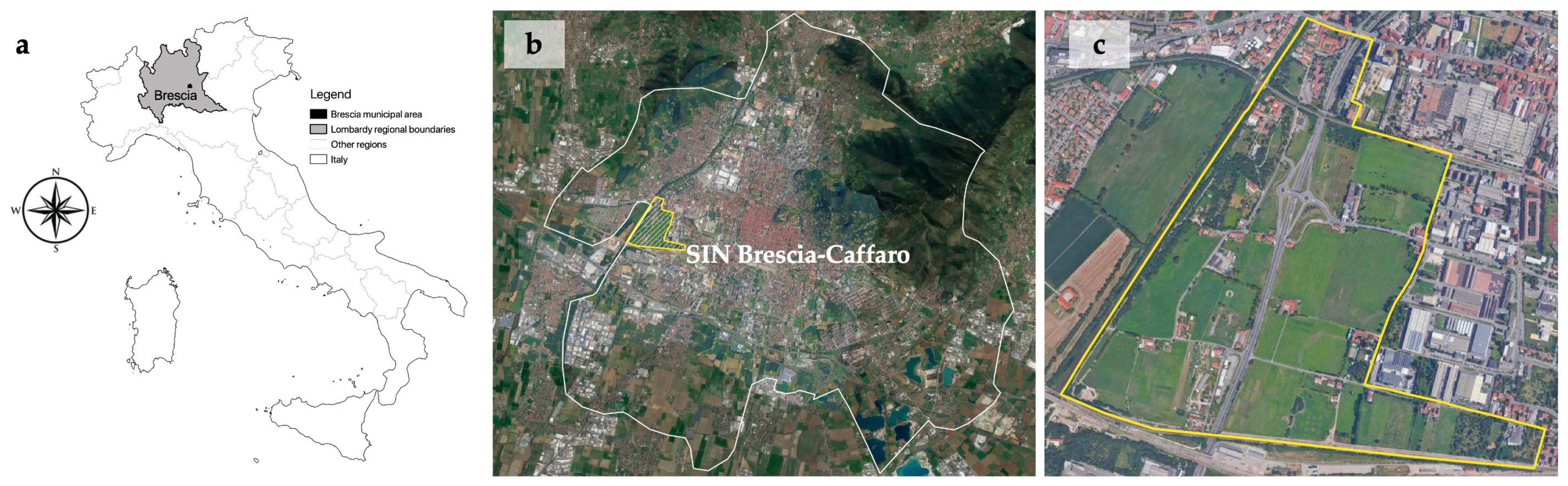

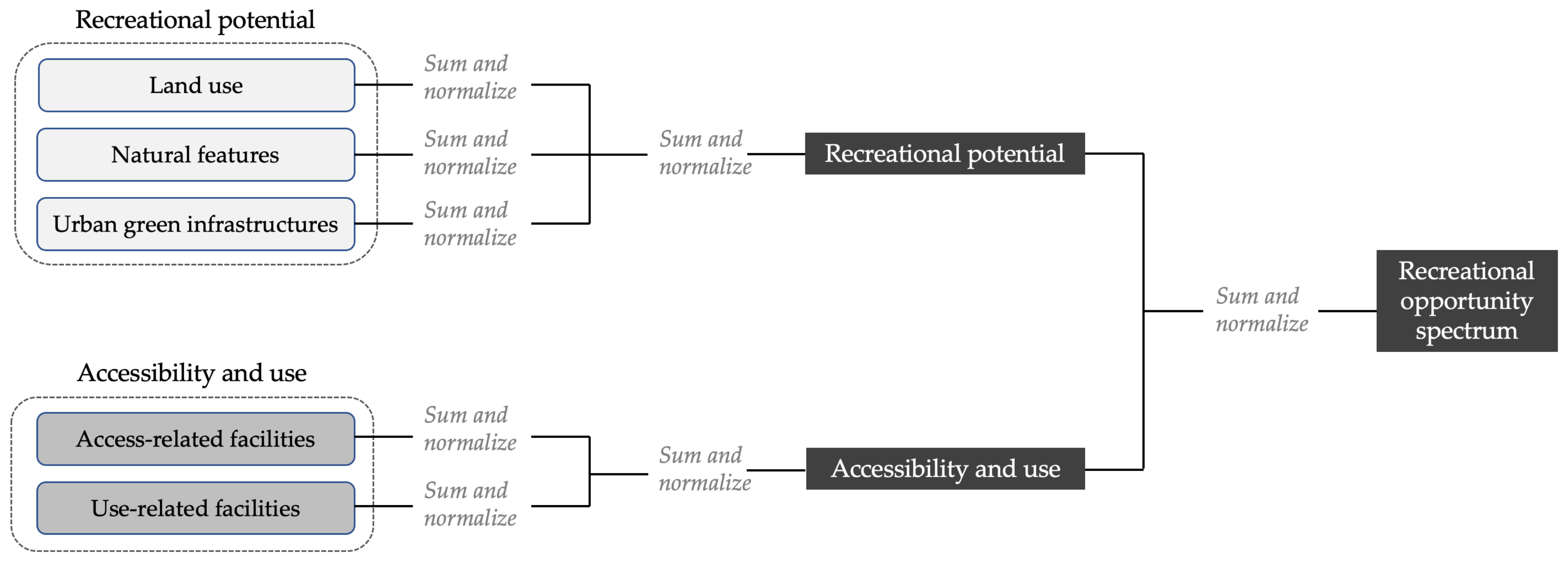


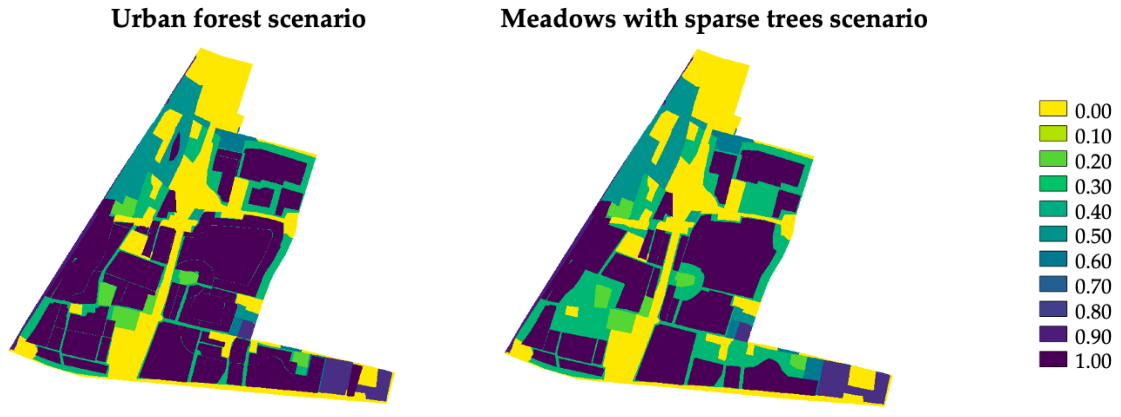

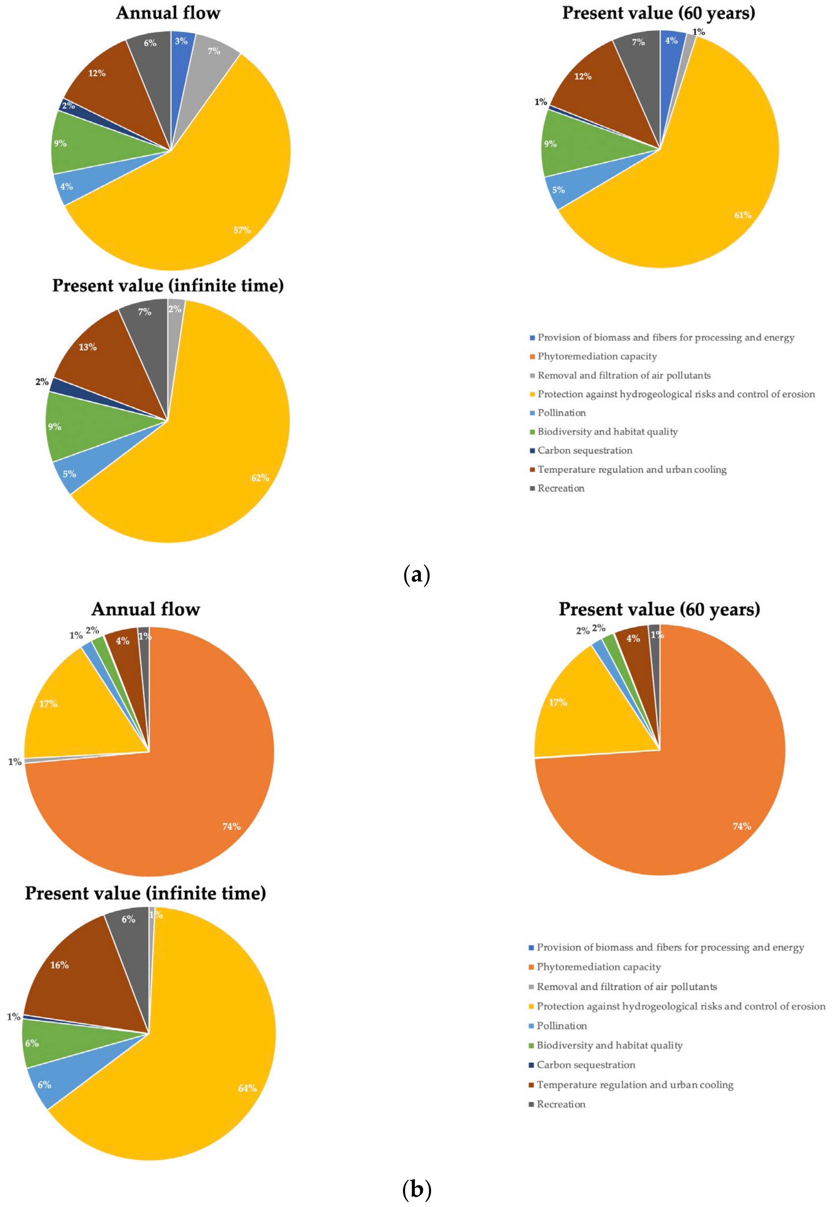
Publisher’s Note: MDPI stays neutral with regard to jurisdictional claims in published maps and institutional affiliations. |
© 2022 by the authors. Licensee MDPI, Basel, Switzerland. This article is an open access article distributed under the terms and conditions of the Creative Commons Attribution (CC BY) license (https://creativecommons.org/licenses/by/4.0/).