Coupling Effects of Precipitation and Vegetation on Sediment Yield from the Perspective of Spatiotemporal Heterogeneity across the Qingshui River Basin of the Upper Yellow River, China

Abstract
:1. Introduction
2. Materials and Methods
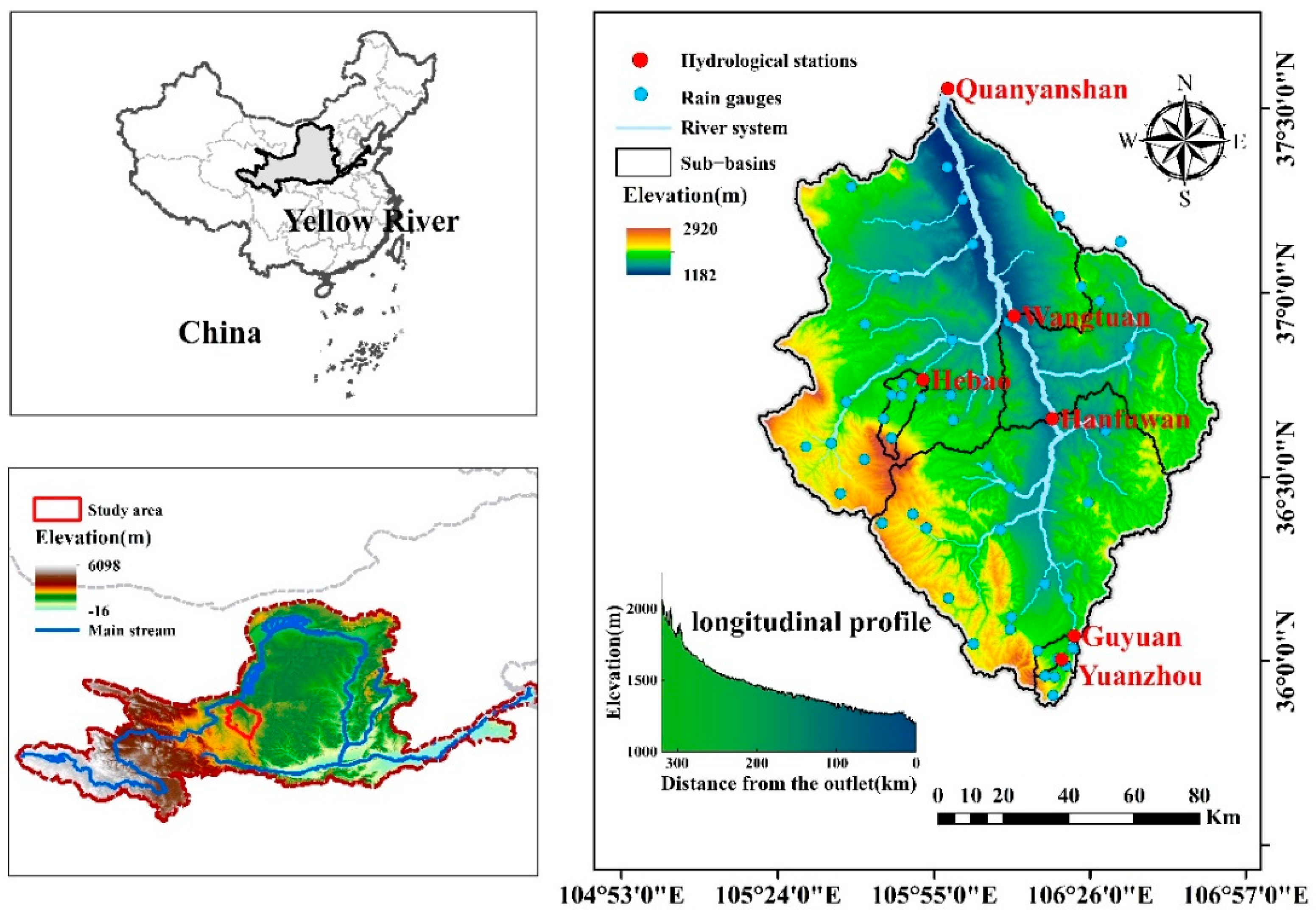
2.1. Study Area
2.2. Data Collection and Processing
2.2.1. Discharge and Sediments
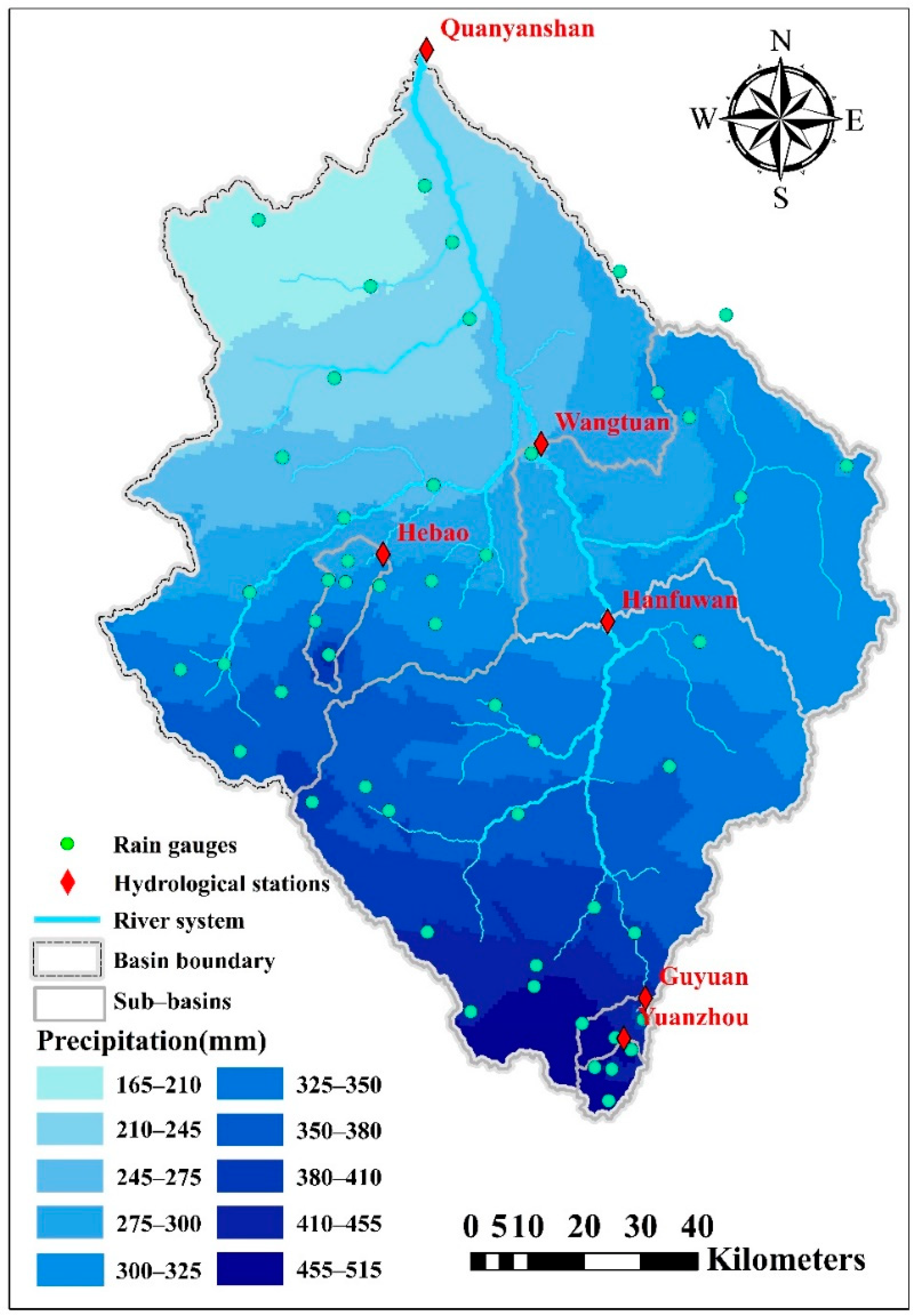
2.2.2. Precipitation
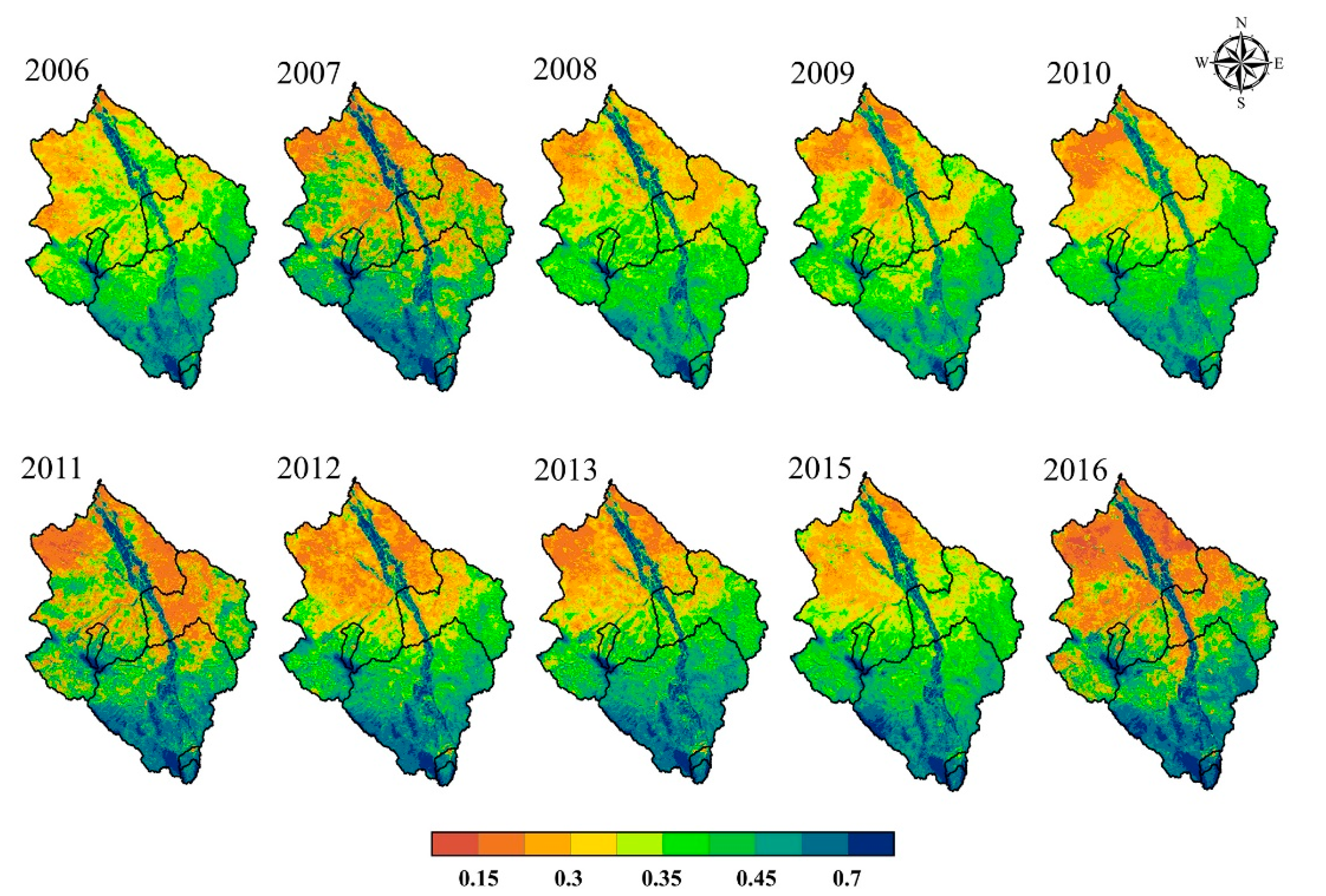
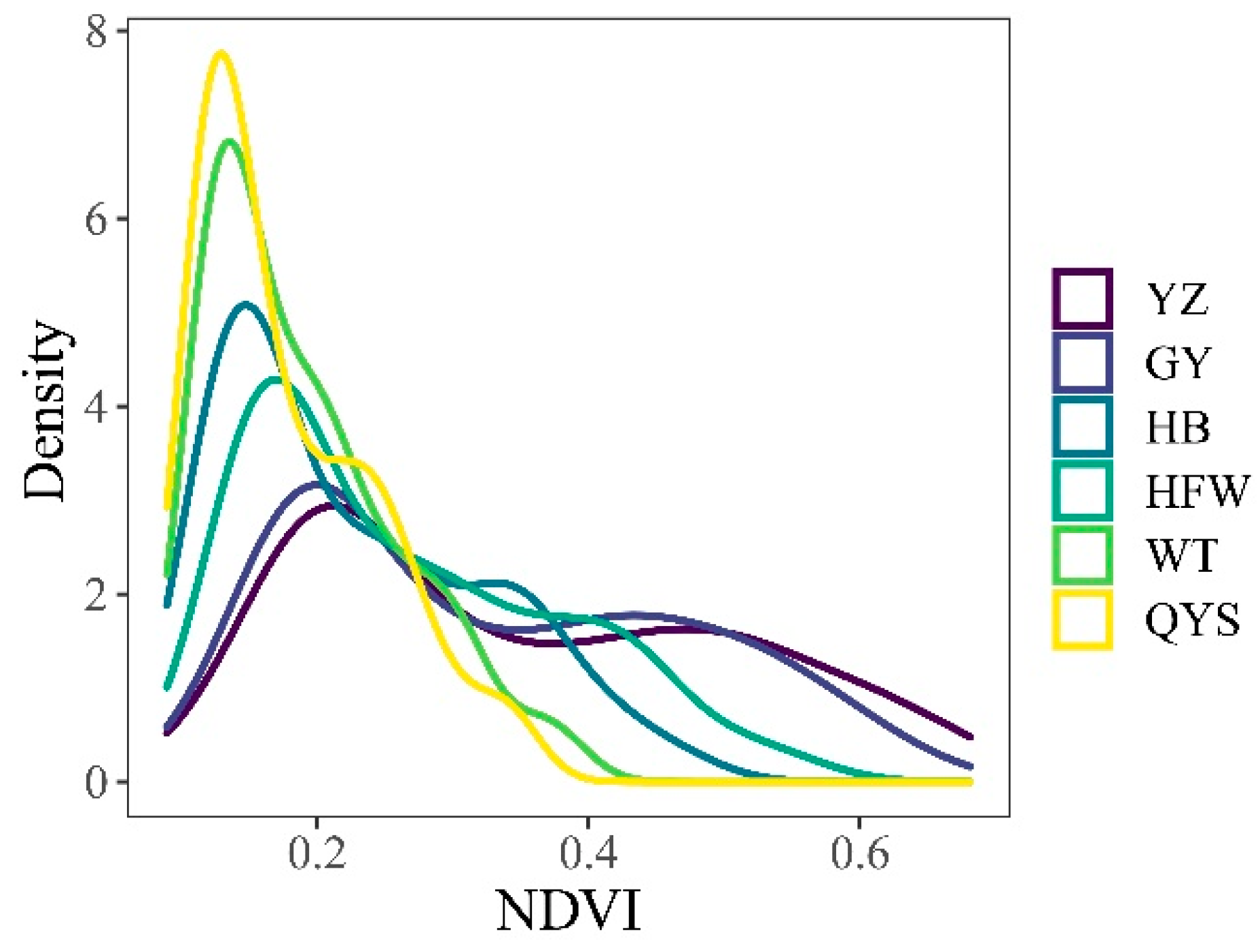
2.2.3. NDVI
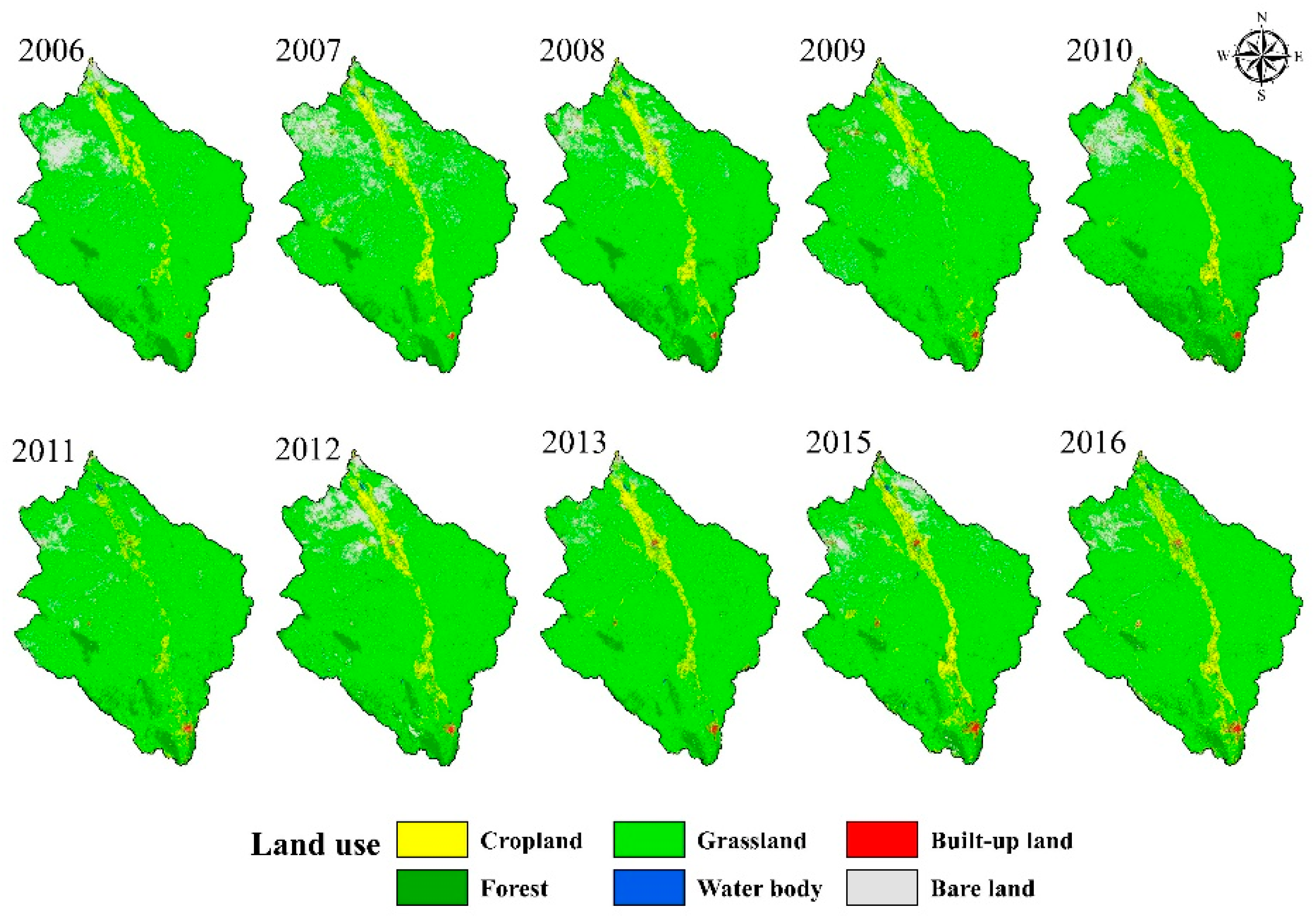
2.2.4. Land Use
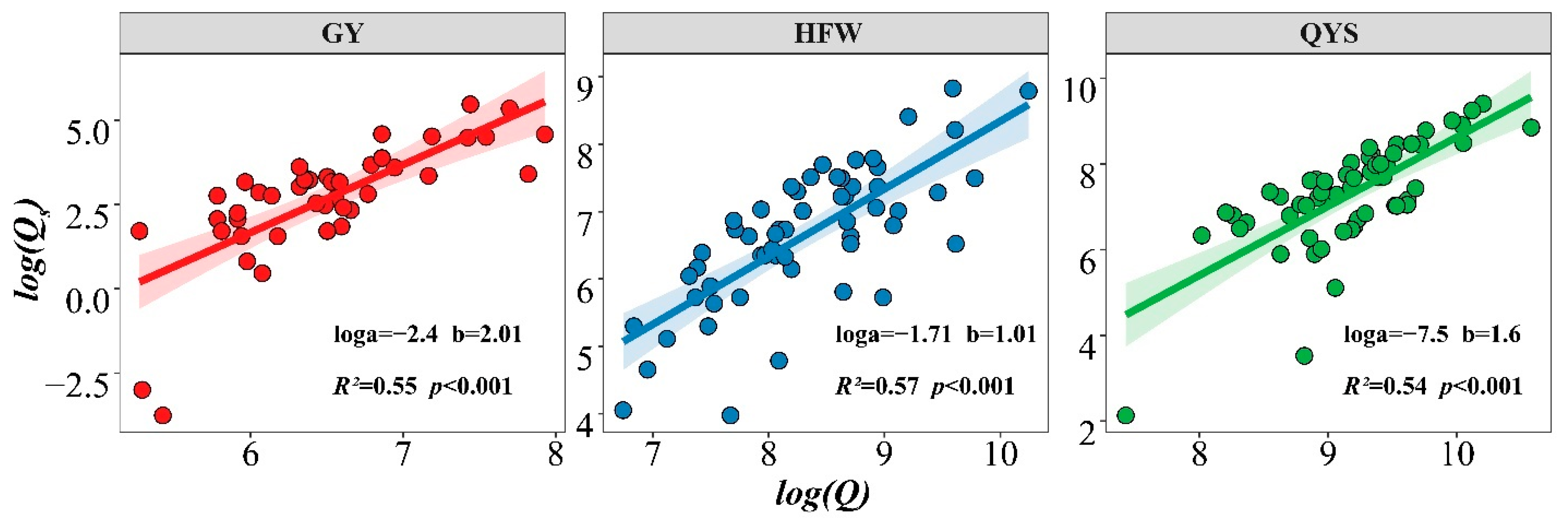
2.3. Sediment Rating Curves (SRCs)
2.4. Trend Analysis
2.5. Precipitation-Vegetation Coupling
2.6. Correlation Analysis
3. Results
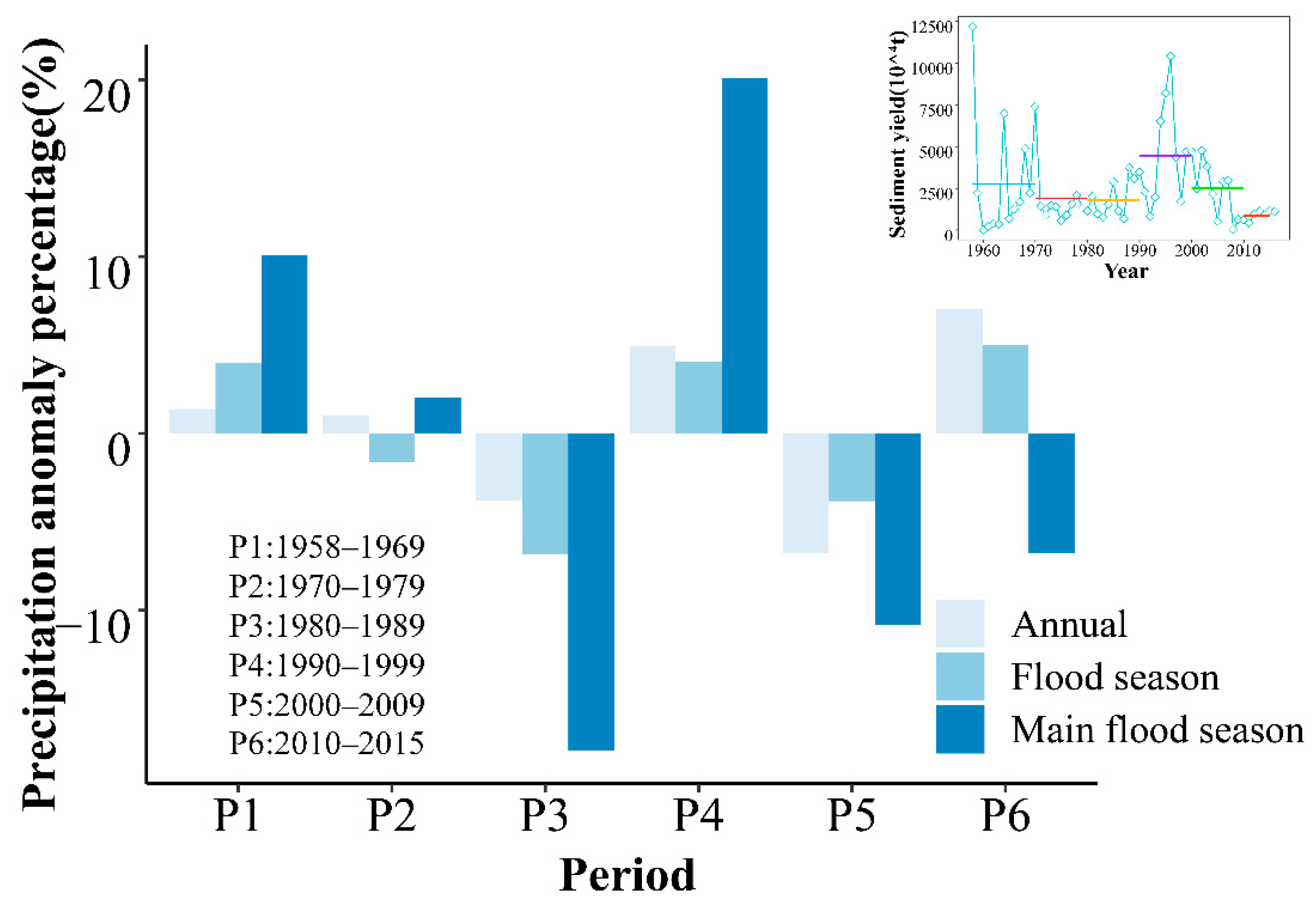
3.1. Trends of River Runoff and Sediment Discharge
3.2. Relationships between River Runoff and Sediment and the Evolution
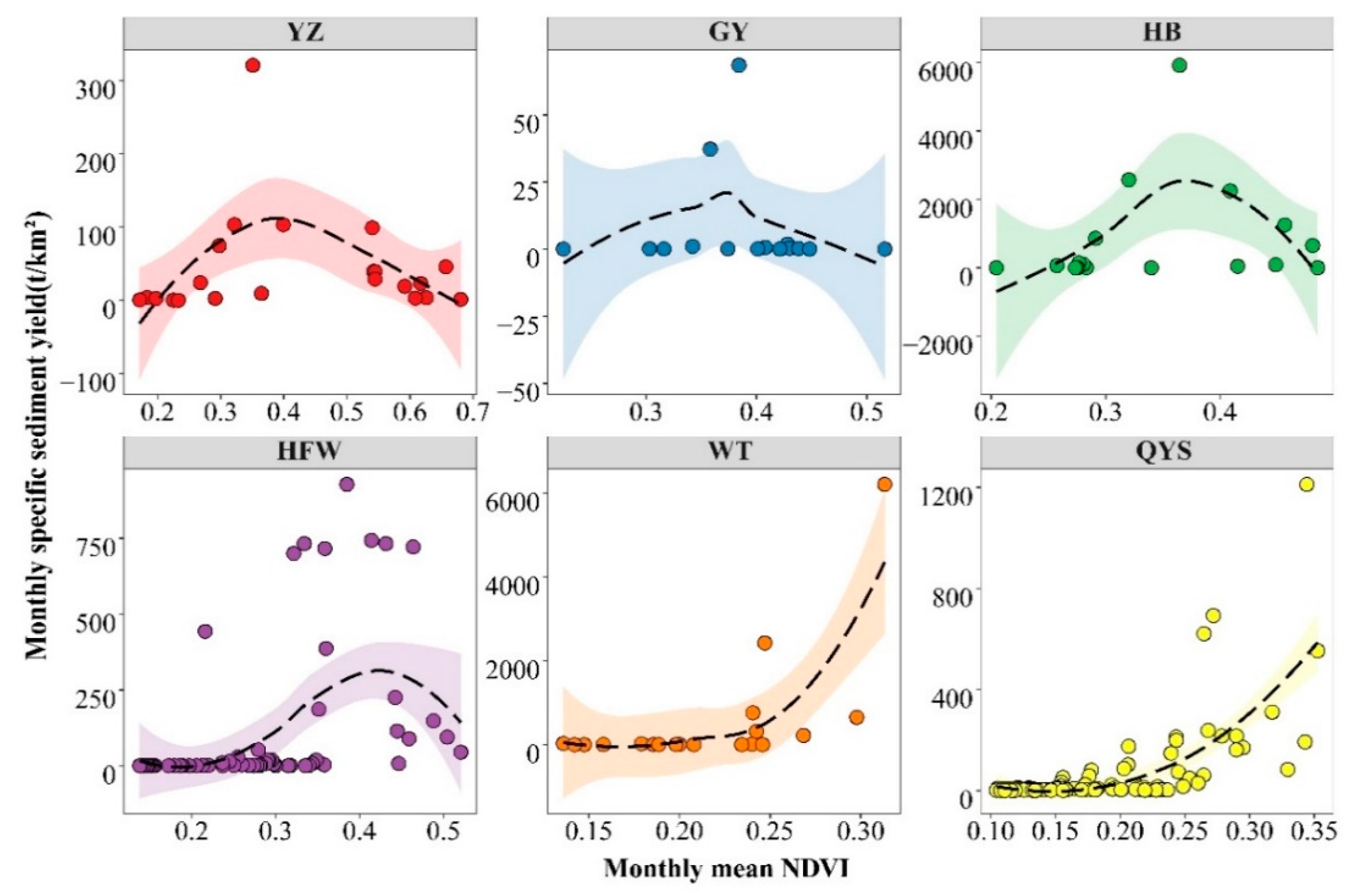
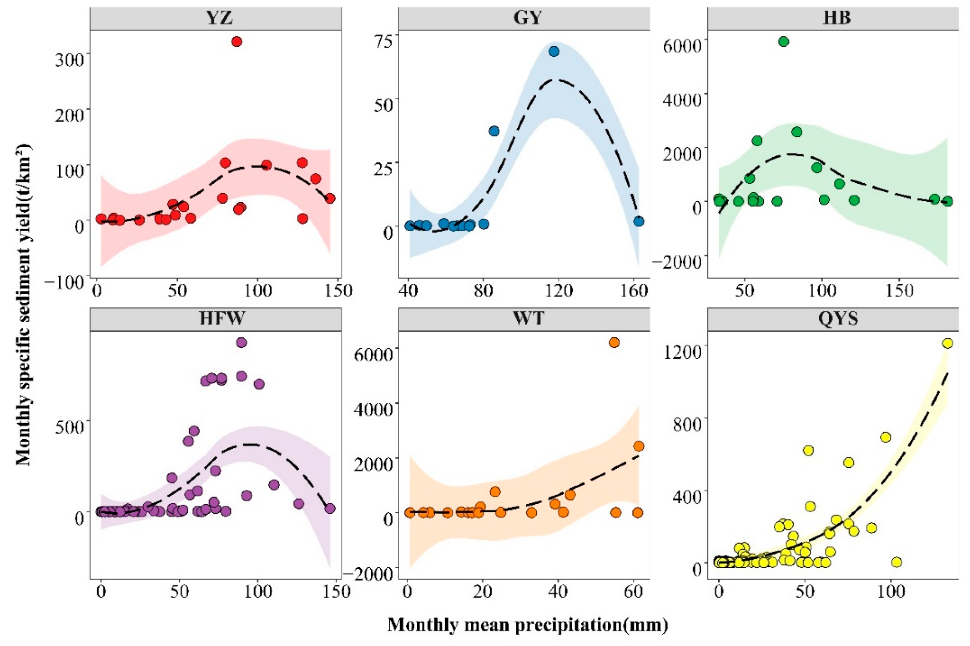
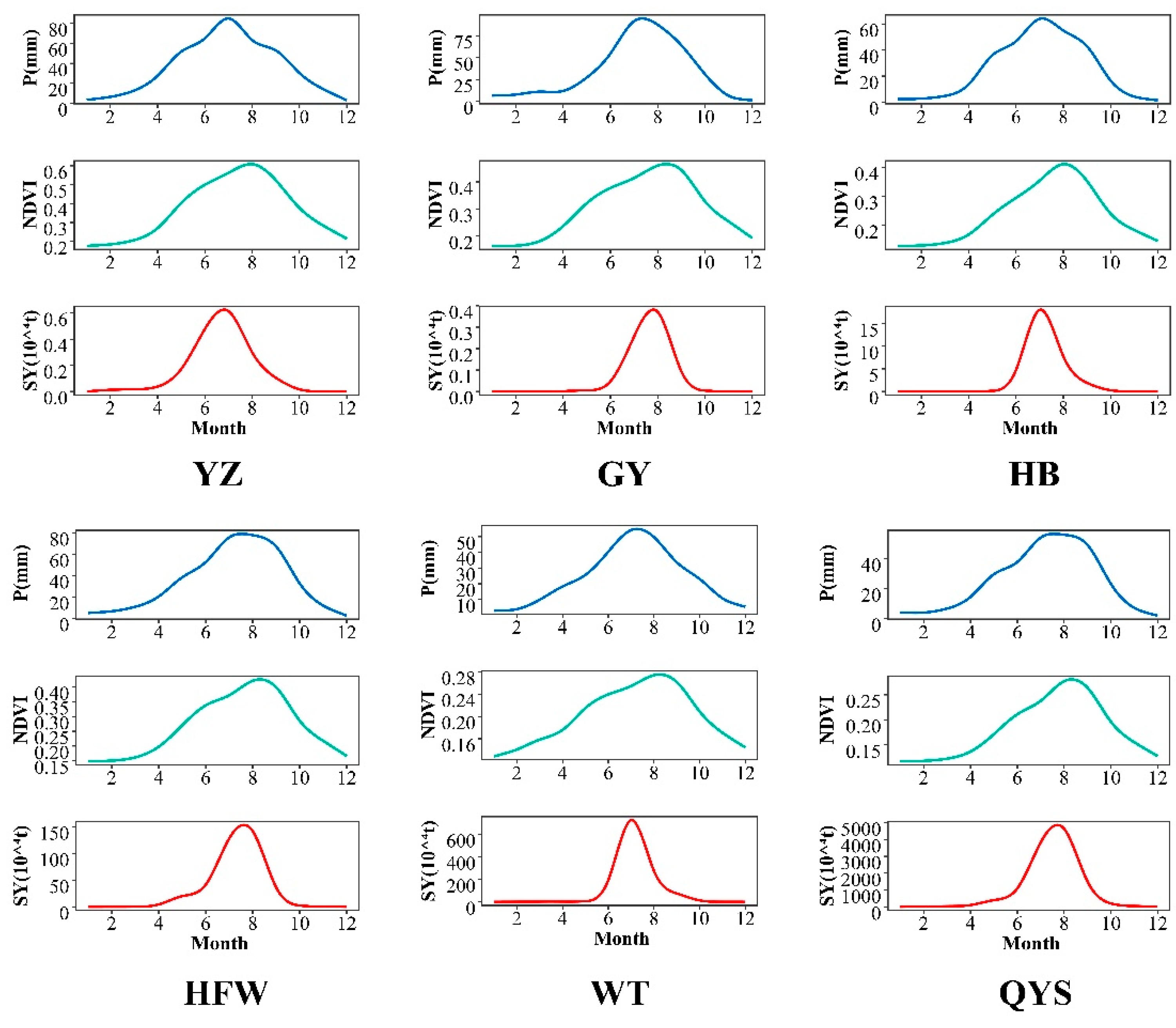
3.3. Relationship between Precipitation, Vegetation, and Erosion
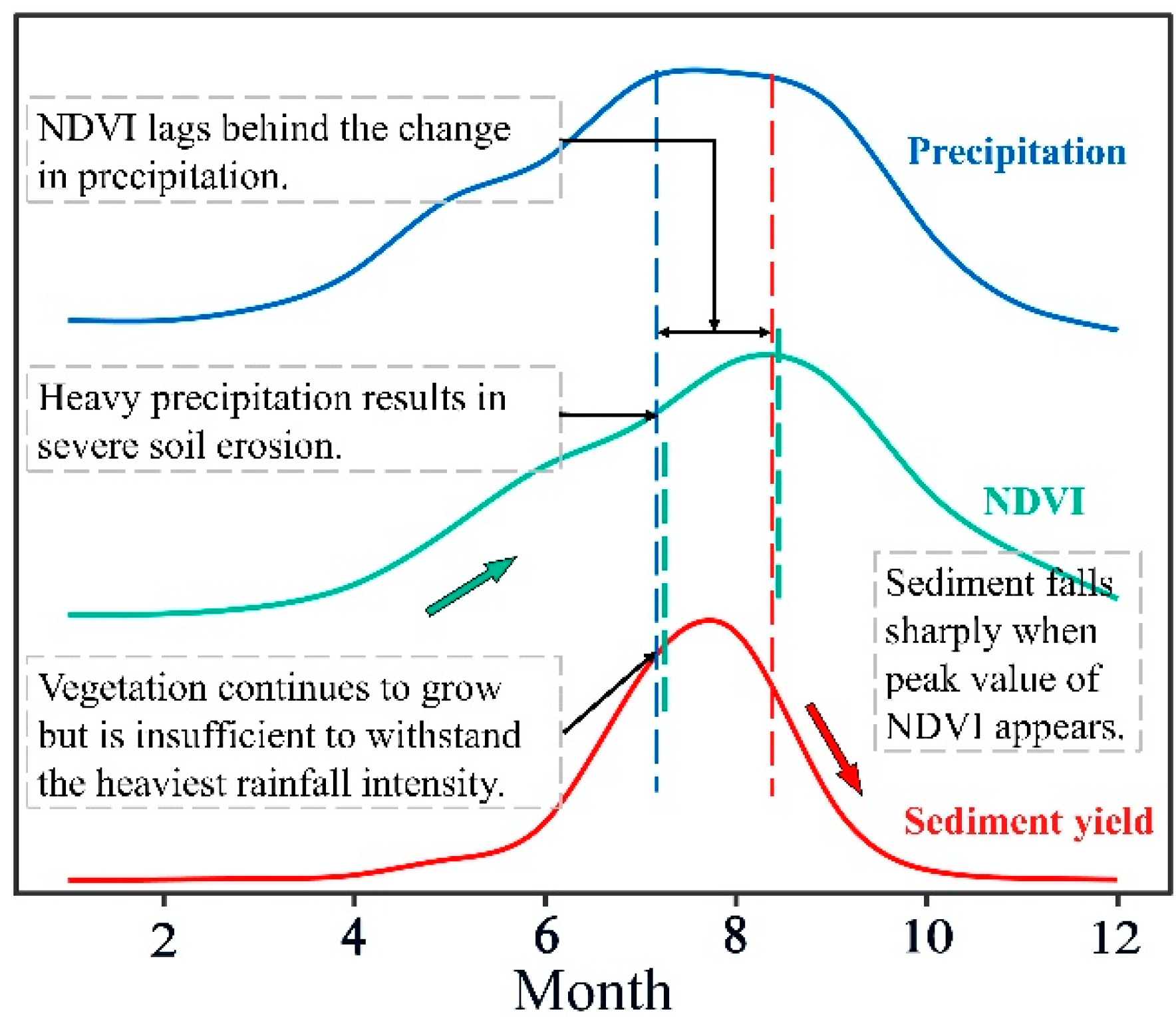
3.4. Time Lag Effect of Vegetation Response to Precipitation
4. Discussion
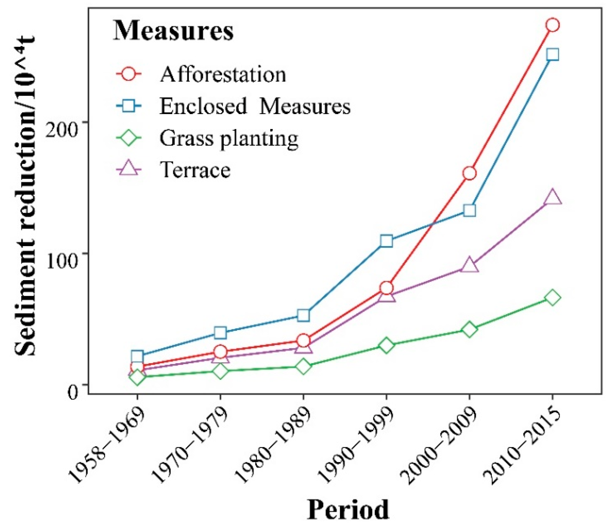
4.1. Possible Drivers of Change in the Discharge–Sediment Relationships
4.2. Response of Sediment to the Coupling Effect of Vegetation and Precipitation
4.3. Potential Influence of NDVI Lags on Sediment Yield in the QRB
5. Conclusions
Author Contributions
Funding
Institutional Review Board Statement
Informed Consent Statement
Data Availability Statement
Acknowledgments
Conflicts of Interest
References
- Walling, D.E.; Fang, D. Recent trends in the suspended sediment loads of the world’s rivers. Glob. Planet Chang. 2003, 39, 111–126. [Google Scholar] [CrossRef]
- Syvitski, J.P.M. Supply and flux of sediment along hydrological pathways: Research for the 21st century. Glob. Planet Chang. 2003, 39, 1–11. [Google Scholar] [CrossRef]
- Wang, S.; Fu, B.; Piao, S.; Lü, Y.; Ciais, P.; Feng, X.; Wang, Y. Reduced sediment transport in the Yellow River due to anthropogenic changes. Nat. Geosci. 2016, 9, 38–41. [Google Scholar] [CrossRef]
- Darby, S.E.; Hackney, C.R.; Leyland, J.; Kummu, M.; Lauri, H.; Parsons, D.R.; Best, J.L.; Nicholas, A.P.; Aalto, R. Fluvial sediment supply to a mega-delta reduced by shifting tropical-cyclone activity. Nature 2016, 539, 276–279. [Google Scholar] [CrossRef] [Green Version]
- Li, L.; Ni, J.; Chang, F.; Yue, Y.; Frolova, N.; Magritsky, D.; Borthwick, A.; Ciais, P.; Wang, Y.; Zheng, C.; et al. Global trends in water and sediment fluxes of the world’s large rivers. Sci. Bull. 2020, 65, 62–69. [Google Scholar] [CrossRef] [Green Version]
- Best, J. Anthropogenic stresses on the world’s big rivers. Nat. Geosci. 2019, 12, 148. [Google Scholar] [CrossRef]
- Ran, Q.; Zong, X.; Ye, S.; Gao, J.; Hong, Y. Dominant mechanism for annual maximum flood and sediment events generation in the Yellow River basin. Catena 2020, 187, 104376. [Google Scholar] [CrossRef]
- Yu, L. The Huanghe (Yellow) River: Recent changes and its countermeasures. Cont. Shelf Res. 2006, 26, 2281–2298. [Google Scholar] [CrossRef]
- Shen, H.; Zheng, F.; Wen, L.; Han, Y.; Hu, W. Impacts of rainfall intensity and slope gradient on rill erosion processes at loessial hillslope. Soil Till. Res. 2016, 155, 429–436. [Google Scholar] [CrossRef]
- Sun, W.; Mu, X.; Song, X.; Wu, D.; Cheng, A.; Qiu, B. Changes in extreme temperature and precipitation events in the Loess Plateau (China) during 1960–2013 under global warming. Atmos. Res. 2016, 168, 33–48. [Google Scholar] [CrossRef]
- Zhao, G.; Mu, X.; Wen, Z.; Wang, F.; Gao, P. Soil erosion, conservation, and eco-environment changes in the Loess Plateau of China. Land Degrad. Dev. 2013, 24, 499–510. [Google Scholar] [CrossRef]
- Chen, L.; Messing, I.; Zhang, S.; Fu, B.; Ledin, S. Land use evaluation and scenario analysis towards sustainable planning on the Loess Plateau in China-case study in a small catchment. Catena 2003, 54, 303–316. [Google Scholar] [CrossRef]
- Han, X.; Xiao, J.; Wang, L.; Tian, S.; Liang, T.; Liu, Y. Identification of areas vulnerable to soil erosion and risk assessment of phosphorus transport in a typical watershed in the Loess Plateau. Sci. Total Environ. 2021, 758, 143661. [Google Scholar] [CrossRef] [PubMed]
- Hessel, R.; Messing, I.; Liding, C.; Ritsema, C.; Stolte, J. Soil erosion simulations of land use scenarios for a small Loess Plateau catchment. Catena 2003, 54, 289–302. [Google Scholar] [CrossRef]
- Zhang, X.; Song, J.; Wang, Y.; Deng, W.; Liu, Y. Effects of land use on slope runoff and soil loss in the Loess Plateau of China: A meta-analysis. Sci. Total Environ. 2021, 755, 142418. [Google Scholar] [CrossRef]
- Fu, B.; Wang, S.; Liu, Y.; Liu, J.; Liang, W.; Miao, C. Hydrogeomorphic ecosystem responses to natural and anthropogenic changes in the Loess Plateau of China. Annu. Rev. Earth Planet Sci. 2017, 45, 223–243. [Google Scholar] [CrossRef]
- Liang, W.; Bai, D.; Wang, F.; Fu, B.; Yan, J.; Wang, S.; Yang, Y.; Long, D.; Feng, M. Quantifying the impacts of climate change and ecological restoration on streamflow changes based on a Budyko hydrological model in China’s Loess Plateau. Water Resour. Res. 2015, 51, 6500–6519. [Google Scholar] [CrossRef]
- Wang, S.; Fu, B.; Liang, W. Developing policy for the Yellow River sediment sustainable control. Natl. Sci. Rev. 2016, 3, 162–164. [Google Scholar] [CrossRef] [Green Version]
- Wang, S.; Fu, B.; Liang, W.; Liu, Y.; Wang, Y. Driving forces of changes in the water and sediment relationship in the Yellow River. Sci. Total Environ. 2017, 576, 453–461. [Google Scholar] [CrossRef]
- Chen, L.; Wei, W.; Fu, B.; Lü, Y. Soil and water conservation on the Loess Plateau in China: Review and perspective. Prog. Phys. Geog. 2007, 31, 389–403. [Google Scholar] [CrossRef]
- Shi, C.; Zhou, Y.; Fan, X.; Shao, W. A study on the annual runoff change and its relationship with water and soil conservation practices and climate change in the middle Yellow River basin. Catena 2013, 100, 31–41. [Google Scholar] [CrossRef]
- Yang, X.; Sun, W.; Li, P.; Mu, X.; Gao, P.; Zhao, G. Reduced sediment transport in the Chinese Loess Plateau due to climate change and human activities. Sci. Total Environ. 2018, 642, 591–600. [Google Scholar] [CrossRef] [PubMed]
- Chen, H.; Cai, Q. Impact of hillslope vegetation restoration on gully erosion induced sediment yield. Sci. China Ser. D 2006, 49, 176–192. [Google Scholar] [CrossRef]
- Chen, H.; Zhou, J.; Cai, Q.; Yue, Z.; Lu, Z.; Liang, G.; Huang, J. The impact of vegetation restoration on erosion-induced sediment yield in the middle Yellow River and management prospect. Sci. China Ser. D 2005, 48, 724–741. [Google Scholar] [CrossRef]
- Liu, X.; Yang, S.; Dang, S.; Luo, Y.; Li, X.; Zhou, X. Response of sediment yield to vegetation restoration at a large spatial scale in the Loess Plateau. Sci. China Technol. Sci. 2014, 57, 1482–1489. [Google Scholar] [CrossRef]
- Murray, S.J.; Foster, P.N.; Prentice, I.C. Future global water resources with respect to climate change and water withdrawals as estimated by a dynamic global vegetation model. J. Hydrol. 2012, 448, 14–29. [Google Scholar] [CrossRef]
- Hu, J.; Gao, P.; Mu, X.; Zhao, G.; Sun, W.; Li, P.; Zhang, L. Runoff-sediment dynamics under different flood patterns in a Loess Plateau catchment, China. Catena 2019, 173, 234–245. [Google Scholar] [CrossRef]
- Xu, J. Precipitation-vegetation coupling and its influence on erosion on the Loess Plateau, China. Catena 2005, 64, 103–116. [Google Scholar]
- Houborg, R.; Boegh, E. Mapping leaf chlorophyll and leaf area index using inverse and forward canopy reflectance modeling and SPOT reflectance data. Remote Sens. Environ. 2008, 112, 186–202. [Google Scholar] [CrossRef]
- Huang, X.; Fang, N.; Shi, Z.; Zhu, T.; Wang, L. Decoupling the effects of vegetation dynamics and climate variability on watershed hydrological characteristics on a monthly scale from subtropical China. Agric. Ecosyst. Environ. 2019, 279, 14–24. [Google Scholar] [CrossRef]
- Rammig, A.; Wiedermann, M.; Donges, J.F.; Babst, F.; von Bloh, W.; Frank, D.; Thonicke, K.; Mahecha, M.D. Coincidences of climate extremes and anomalous vegetation responses: Comparing tree ring patterns to simulated productivity. Biogeosciences 2015, 12, 373–385. [Google Scholar] [CrossRef] [Green Version]
- Zhao, A.; Zhang, A.; Liu, X.; Cao, S. Spatiotemporal changes of normalized difference vegetation index (NDVI) and response to climate extremes and ecological restoration in the Loess Plateau, China. Theor. Appl. Climatol. 2018, 132, 555–567. [Google Scholar] [CrossRef]
- Reyer, C.P.; Silveyra Gonzalez, R.; Dolos, K.; Hartig, F.; Hauf, Y.; Noack, M.; Lasch-Born, P.; Rötzer, T.; Pretzsch, H.; Meesenburg, H.; et al. The PROFOUND Database for evaluating vegetation models and simulating climate impacts on European forests. Earth Syst. Sci. Data 2020, 12, 1295–1320. [Google Scholar] [CrossRef]
- Ding, Y.; Li, Z.; Peng, S. Global analysis of time-lag and -accumulation effects of climate on vegetation growth. Int. J. Appl. Earth Obs. 2020, 92, 102179. [Google Scholar] [CrossRef]
- Tian, S.; Xu, M.; Jiang, E.; Wang, G.; Hu, H.; Liu, X. Temporal variations of runoff and sediment load in the upper Yellow River, China. J. Hydrol. 2019, 568, 46–56. [Google Scholar] [CrossRef]
- Jiao, P.; Wei, W.; Bao, H. Variation and Trend Analysis of Rainfall in Qingshui River Basin of Ningxia in China, IOP Conference Series: Earth and Environmental Science. IOP Publ. 2020, 526, 012040. [Google Scholar]
- Zhao, Y.; Cao, W.; Hu, C. Analysis of changes in characteristics of flood and sediment yield in typical basins of the Yellow River under extreme rainfall events. Catena 2019, 177, 31–40. [Google Scholar] [CrossRef]
- Li, C.; Zhang, H.; Singh, V.P.; Fan, J.; Wei, X.; Yang, J.; Wei, X. Investigating variations of precipitation concentration in the transitional zone between Qinling Mountains and Loess Plateau in China: Implications for regional impacts of AO and WPSH. PLoS ONE 2020, 15, e0238709. [Google Scholar] [CrossRef]
- Shi, S.; Yu, J.; Wang, F.; Wang, P.; Zhang, Y.; Jin, K. Quantitative contributions of climate change and human activities to vegetation changes over multiple time scales on the Loess Plateau. Sci. Total Environ. 2021, 755, 142419. [Google Scholar] [CrossRef]
- Ahn, K.H.; Steinschneider, S. Time-varying suspended sediment-discharge rating curves to estimate climate impacts on fluvial sediment transport. Hydrol. Process. 2018, 32, 102–117. [Google Scholar] [CrossRef]
- De Girolamo, A.M.; Pappagallo, G.; Lo Porto, A. Temporal variability of suspended sediment transport and rating curves in a Mediterranean river basin: The Celone (SE Italy). Catena 2015, 128, 135–143. [Google Scholar] [CrossRef]
- Khaleghi, M.R.; Varvani, J. Sediment Rating Curve Parameters Relationship with Watershed Characteristics in the Semiarid River Watersheds. Arab. J. Sci. Eng. 2018, 43, 3725–3737. [Google Scholar] [CrossRef]
- Zhang, W.; Wei, X.; Zheng, J.; Zhu, Y.; Zhang, Y. Estimating suspended sediment loads in the Pearl River Delta region using sediment rating curves. Cont. Shelf Res. 2012, 38, 35–46. [Google Scholar] [CrossRef]
- Hu, B.; Wang, H.; Yang, Z.; Sun, X. Temporal and spatial variations of sediment rating curves in the Changjiang (Yangtze River) basin and their implications. Quatern. Int. 2011, 230, 34–43. [Google Scholar] [CrossRef]
- Warrick, J.A. Trend analyses with river sediment rating curves. Hydrol. Process. 2015, 29, 936–949. [Google Scholar] [CrossRef]
- Kendall, M. Rank Correlation Methods; Charles Griffin: London, UK, 1975. [Google Scholar]
- Mann, H.B. Nonparametric tests against trend. Econom. J. Econom. Soc. 1945, 245–259. [Google Scholar] [CrossRef]
- Sen, P.K. Estimates of the regression coefficient based on Kendall’s tau. J. Am. Stat. Assoc. 1968, 63, 1379–1389. [Google Scholar] [CrossRef]
- Chu, H.; Venevsky, S.; Wu, C.; Wang, M. NDVI-based vegetation dynamics and its response to climate changes at Amur-Heilongjiang River Basin from 1982 to 2015. Sci. Total Environ. 2019, 650, 2051–2062. [Google Scholar] [CrossRef]
- Li, J.; Peng, S.; Li, Z. Detecting and attributing vegetation changes on China’s Loess Plateau. Agric. Forest Meteorol. 2017, 247, 260–270. [Google Scholar] [CrossRef]
- Xin, Z.; Yu, X.; Lu, X. Factors controlling sediment yield in China’s Loess Plateau. Earth Surf. Proc. Land. 2011, 36, 816–826. [Google Scholar] [CrossRef]
- Ye, S.; Ran, Q.; Fu, X.; Hu, C.; Wang, G.; Parker, G.; Chen, X.; Zhang, S. Emergent stationarity in Yellow River sediment transport and the underlying shift of dominance: From streamflow to vegetation. Hydrol. Earth Syst. Sci. 2019, 23, 549–556. [Google Scholar] [CrossRef] [Green Version]
- Rundquist, B.C.; Harrington, J.A., Jr. The effects of climatic factors on vegetation dynamics of tallgrass and shortgrass cover. Geocarto. Int. 2000, 15, 33–38. [Google Scholar] [CrossRef]
- Zhao, J.; Huang, S.; Huang, Q.; Wang, H.; Leng, G.; Fang, W. Time-lagged response of vegetation dynamics to climatic and teleconnection factors. Catena 2020, 189, 104474. [Google Scholar] [CrossRef]
- Wang, H.; Sun, F. Variability of annual sediment load and runoff in the Yellow River for the last 100 years (1919–2018). Sci. Total Environ. 2021, 758, 143715. [Google Scholar] [CrossRef]
- Zheng, K.; Wei, J.; Pei, J.; Cheng, H.; Zhang, X.; Huang, F.; Li, F.; Ye, J. Impacts of climate change and human activities on grassland vegetation variation in the Chinese Loess Plateau. Sci. Total Environ. 2019, 660, 236–244. [Google Scholar] [CrossRef] [PubMed]
- Duan, J.; Liu, Y.; Tang, C.; Shi, Z.; Yang, J. Efficacy of orchard terrace measures to minimize water erosion caused by extreme rainfall in the hilly region of China: Long-term continuous in situ observations. J. Environ. Manag. 2021, 278, 11537. [Google Scholar] [CrossRef] [PubMed]
- Mukai, S.; Billi, P.; Haregeweyn, N.; Hordofa, T. Long-term effectiveness of indigenous and introduced soil and water conservation measures in soil loss and slope gradient reductions in the semi-arid Ethiopian lowlands. Geoderma 2021, 382, 114757. [Google Scholar] [CrossRef]
- Wang, T.; Hou, J.; Li, P.; Zhao, J.; Li, Z.; Matta, E.; Ma, L.; Hinkelmann, R. Quantitative assessment of check dam system impacts on catchment flood characteristics-a case in hilly and gully area of the Loess Plateau, China. Nat. Hazards 2021, 105, 3059–3077. [Google Scholar] [CrossRef]
- Sun, P.; Wu, Y.; Yang, Z.; Sivakumar, B.; Qiu, L.; Liu, S.; Cai, Y. Can the Grain-for-Green Program really ensure a low sediment load on the Chinese Loess Plateau? Engineering 2019, 5, 855–864. [Google Scholar] [CrossRef]
- Li, Y.; Jiao, P.; Zhang, X.; Yang, J.; Wei, W. Change of precipitation and sediment of Qingshui River Basin of Ningxia in recent 60 years. Res. Soil Water Conserv. 2021, 28, 184–189. [Google Scholar]
- Zheng, M. A spatially invariant sediment rating curve and its temporal change following watershed management in the Chinese Loess Plateau. Sci. Total Environ. 2018, 630, 1453–1463. [Google Scholar] [CrossRef]
- Gao, G.; Fu, B.; Zhang, J.; Ma, Y.; Sivapalan, M. Multiscale temporal variability of flow-sediment relationships during the 1950s-2014 in the Loess Plateau, China. J. Hydrol. 2018, 563, 609–619. [Google Scholar] [CrossRef]
- Atieh, M.; Mehltretter, S.L.; Gharabaghi, B.; Rudra, R. Integrative neural networks model for prediction of sediment rating curve parameters for ungauged basins. J. Hydrol. 2015, 531, 1095–1107. [Google Scholar] [CrossRef]
- Zhang, S.; Chen, D.; Li, F.; He, L.; Yan, M.; Yan, Y. Evaluating spatial variation of suspended sediment rating curves in the middle Yellow River basin, China. Hydrol. Process. 2018, 32, 1616–1624. [Google Scholar] [CrossRef]
- Langbein, W.B.; Schumm, S.A. Yield of sediment in relation to mean annual precipitation. Eos Trans. Am. Geophys. Union 1958, 39, 1076–1084. [Google Scholar] [CrossRef] [Green Version]
- Douglas, I. Man, vegetation and the sediment yields of rivers. Nature 1967, 215, 925–928. [Google Scholar] [CrossRef]
- Rogers, R.; Schumm, S.A. The effect of sparse vegetative cover on erosion and sediment yield. J. Hydrol. 1991, 123, 19–24. [Google Scholar] [CrossRef]
- Corenblit, D.; Steiger, J.; Gurnell, A.M.; Tabacchi, E.; Roques, L. Control of sediment dynamics by vegetation as a key function driving biogeomorphic succession within fluvial corridors. Earth Surf. Proc. Land. 2009, 34, 1790–1810. [Google Scholar] [CrossRef]
- Ning, T.; Liu, W.; Lin, W.; Song, X. NDVI Variation and its responses to Climate Change on the Northern Loess Plateau of China from 1998 to 2012. Adv. Meteorol. 2015, 2015, 1–10. [Google Scholar] [CrossRef] [Green Version]
- Kong, D.; Miao, C.; Wu, J.; Zheng, H.; Wu, S. Time lag of vegetation growth on the Loess Plateau in response to climate factors: Estimation, distribution, and influence. Sci. Total. Environ. 2020, 744, 140726. [Google Scholar] [CrossRef] [PubMed]


| Stations | Control Area (km2) | Series (Annual) | Average Discharge (104 m3) | Discharge Range (104 m3) | Average Sediment Yield (104 t) | Sediment Yield Range (104 t) | Series (Daily) | Peak Discharge (m3/s) | Peak Sediment Concentration (kg/s) |
|---|---|---|---|---|---|---|---|---|---|
| YZ | 105 | 2009–2013 2015–2016 | 225 | 26–469 | 1.48 | 0.349–3.98 | 2009–2013 2015–2016 | 48.1 | 381 |
| GY | 105 | 1967–2008 | 824 | 166–2778 | 35.6 | 0.0234–238 | 2006–2008 | 153 | 57.8 |
| HB | 200 | 2006–2013 2015–2016 | 362 | 219–516 | 23.1 | 0.017–119 | 2006–2013 2015–2016 | 354 | 899 |
| HFW | 4935 | 1960–2013 2015–2016 | 5666 | 849–35,100 | 1242 | 53.2–6840 | 2006–2013 2015–2016 | 311 | 967 |
| WT | 2430 | 2015–2016 | 4642 | 4303–4981 | 1294 | 838–1750 | 2015–2016 | 816 | 968 |
| QYS | 7115 | 1955–2013 2015–2016 | 11,473 | 1750–39,200 | 2582 | 8.43–12,200 | 2006–2013 2015–2016 | 230 | 1050 |
| Hydrological Station | Annual Discharge | Annual Sediment Yield | |||
|---|---|---|---|---|---|
| MK, Z | Sen’s, β (104 m3) | MK, Z | Sen’s, β (104 t) | ||
| Guyuan | −3.44 *** | −18.75 | −3.4 *** | −0.66 | |
| Hanfuwan | −5.16 *** | −119.56 | −1.3 NS | −6.86 | |
| Quanyanshan | 1.41 NS | 61.23 | 0.56 NS | 6.62 | |
| Sub-Basins | Lag Month | Precipitation–NDVI | Sub-Basins | Lag Month | Precipitation–NDVI | ||||
|---|---|---|---|---|---|---|---|---|---|
| Spring | Summer | Autumn | Spring | Summer | Autumn | ||||
| GY | 0 | 0.43 | 0.62 | 0.82 ** | HFW | 0 | 0.68 * | 0.59 * | 0.74 *** |
| 1 | 0.2 | 0.85 ** | 0.37 | 1 | 0.76 *** | 0.54 * | 0.43 * | ||
| 2 | 0.27 | 0.67 * | −0.5 | 2 | 0.34 | 0.72 *** | 0.22 | ||
| 3 | 0.07 | 0.22 | −0.56 | 3 | 0.19 | 0.51 * | −0.15 | ||
| YZ | 0 | 0.85 ** | 0.35 | 0.83 *** | WT | 0 | 0.37 | 0.42 | 0.81 * |
| 1 | 0.89 *** | 0.03 | 0.66 ** | 1 | 0.69 * | 0.14 | 0.57 | ||
| 2 | 0.69 ** | 0.51 * | 0.19 | 2 | 0.33 | 0.57 * | −0.47 | ||
| 3 | 0.26 | 0.18 | −0.16 | 3 | −0.52 | −0.05 | −0.76 | ||
| HB | 0 | 0.64 ** | 0.56 * | 0.8 *** | QYS | 0 | 0.6 ** | 0.57 ** | 0.75 *** |
| 1 | 0.75 *** | 0.63 ** | 0.44 * | 1 | 0.68 *** | 0.51 ** | 0.36 * | ||
| 2 | 0.12 | 0.68 *** | 0.21 | 2 | −0.03 | 0.7 *** | 0.27 | ||
| 3 | 0.14 | 0.54 * | −0.28 | 3 | 0.12 | 0.5 | −0.16 | ||
Publisher’s Note: MDPI stays neutral with regard to jurisdictional claims in published maps and institutional affiliations. |
© 2022 by the authors. Licensee MDPI, Basel, Switzerland. This article is an open access article distributed under the terms and conditions of the Creative Commons Attribution (CC BY) license (https://creativecommons.org/licenses/by/4.0/).
Share and Cite
Yang, J.; Zhang, H.; Yang, W. Coupling Effects of Precipitation and Vegetation on Sediment Yield from the Perspective of Spatiotemporal Heterogeneity across the Qingshui River Basin of the Upper Yellow River, China. Forests 2022, 13, 396. https://doi.org/10.3390/f13030396
Yang J, Zhang H, Yang W. Coupling Effects of Precipitation and Vegetation on Sediment Yield from the Perspective of Spatiotemporal Heterogeneity across the Qingshui River Basin of the Upper Yellow River, China. Forests. 2022; 13(3):396. https://doi.org/10.3390/f13030396
Chicago/Turabian StyleYang, Jun, Huilan Zhang, and Weiqing Yang. 2022. "Coupling Effects of Precipitation and Vegetation on Sediment Yield from the Perspective of Spatiotemporal Heterogeneity across the Qingshui River Basin of the Upper Yellow River, China" Forests 13, no. 3: 396. https://doi.org/10.3390/f13030396
APA StyleYang, J., Zhang, H., & Yang, W. (2022). Coupling Effects of Precipitation and Vegetation on Sediment Yield from the Perspective of Spatiotemporal Heterogeneity across the Qingshui River Basin of the Upper Yellow River, China. Forests, 13(3), 396. https://doi.org/10.3390/f13030396